Exact Inference of Hidden Structure from Sample Data in Noisy-OR Networks

Michael Kearns AT&T Labs

180 Park Avenue, Room A235 Florham Park, New Jersey 07932 [email protected]

1 Introduction

In the literature on graphical models, there has been increased attention paid to the problems of learning hidden structure (see Heckerman (H96] for a survey) and causal mechanisms from sample data (H96, P88, S93, P95, F98]. In most settings we should expect the former to be difficult, and the latter potentially impossible without experimental intervention. In this work, we examine some restricted settings in which the ideal can be obtained: efficient algorithms that perfectly reconstruct the hidden structure solely on the basis of observed sample data.

In our framework, we assume that the unknown "tar­ get" network is a two-layer, noisy-OR network meeting a number of assumptions detailed in the paper; briefly, the assumptions limit the "fan-in" of each output node (the number of inputs that can influence that node) and the number of possible values for the weights in the network. Learning algorithms observe indepen­ dent draws of the output units only; the values of the input units are always unobserved. Rather than just approximate the output distribution (a perfectly rea­ sonable goal), our algorithms exactly reconstruct the directed graph from the inputs to the outputs (the hid­ den structure), and do so in time polynomial in the size of the target network (and other parameters detailed below).

There are two main ideas behind our algorithms:

• The integration of accurate structural information about many "small subnetworks" of the target network in order to obtain the correct structure for the entire network.
• The acquisition of accurate structural information about the small subnetworks from the passively observed values on the outputs.

Yishay Mansour

Tel Aviv University Department of Computer Science Tel Aviv, Israel mansour@math. tau.ac.il

The strength of our results is indicative of the strength of our assumptions, as we do not expect results of this type to be possible in all but the most fortunate situa­ tions. Nevertheless, the assumptions do not trivialize the problem - there are still exponentially many net­ works meeting our restrictions and we hope that some of the underlying mathematical tools we intro­ duce may lead to more widely applicable heuristics.

The outline of the paper is as follows. In Section 2, we give definitions for the types of networks we ex­ amine, and introduce the restrictions on them that we will require. In Section 3, we introduce an ab­ straction that we call Subnetwork Equivalence Queries that allows us to describe the first main idea behind our algorithms, the integration of accurate structural information about many small pieces of the unknown network. Section 4 examines the conditions required to implement such queries from sample data, and gives the overall description of our algorithms.

2 Definitions and Preliminaries

We will use the standard definitions for two-layer noisy-OR belief networks. Such a network has n in­ puts X1, . .. , Xn and m outputs Y1, . .. , Ym. For each input Xi and output }j there is an associated weight 'f/ i j E (0, 1] , and we say that Xi and }j are connected if and only if 'f/ i j 'I 1. In our framework, the inputs Xi will be hidden variables, whose values are never ob­ served in the data available to our learning algorithms. The outputs }j will be fully observable.

With each output Yj we associate the set Sj of (indices of) inputs Xi that are connected to }j, and we say the network has fan-in kif IS; I � k for all 1 � i � m.

We use the standard definition for the conditional dis-

tribution of lj given values for its parents:

Another way of describing the way such a network gen­ erates a distribution on its outputs, given values for the inputs, is as follows. We associate with each input Xi and output lj that are connected a binary random variable Rij, where Pr[Rij = OJ = 7Jij. The output variable lj is set to

Thus, we define a noisy-OR network N to consist of the connection parameters 7lii between every input Xi and output lj. The network N does not yet specify a probability distribution; to specify the joint distribu­ tion defined by N it remains only to assign indepen­ dent biases Pi to the input units Xi. In this paper, we will restrict our attention to distributions obtained by setting all of the Pi to some common value p, and we shall denote the resulting joint distribution on the outputs lj by Np.

With the networks of interest now specified, we can describe the learning model we will study. Our learn­ ing algorithms will be given independent output draws from a distribution defined by an unknown two-layer noisy-OR target network Np. Each draw observed by the learning algorithm consists of values for the outputs Y1, . . . , Yn only -the values for the inputs X1, ... , Xm that generated the observed outputs are always hidden. In the terminology of the graphical models literature, we are in the partially observed data, unknown structure setting.

A perfectly reasonable goal for a learning algorithm in this setting would be to use the data to learn an ap­ proximation of the unknown target distribution over the lj only, since these are the only variables that are observed. In such a model, we do not ask the learn­ ing algorithm to explicitly derive the assumed causal relationships between the Xi and the lj. Indeed, the learning algorithm is free to not represent the xi at all, since only an accurate approximation of the out­ put distribution is required. There are many works that either implicitly or explicitly take this view of distribution learning. The closest in spirit to the cur­ rent work is [K94J, in which a "PAC-like" model for distribution learning was formalized.

In this paper, however, we study a much more de­ manding criterion for learning. Under some strong as­ sumptions on the unknown target network generating the observed output draws, we give algorithms that will, with high probability, exactly recover the struc­ ture of the target network, and furthermore, will do so in time polynomial in the size of the target net­ work. Thus, not only will the resulting approximation of the output distribution be perfect (Kullback-Leibler divergence 0 to the target distribution), but the true underlying directed graph of the target network will be inferred. This can be viewed as a demonstration of a restricted setting in which it is in fact possible to recover the exact structure on the basis of passively ob­ served data, a task that under general circumstances is difficult or impossible.

As the reader will suspect, in order to obtain such strong results, we will require a number of restrictions on the general two-layer noisy-OR networks we have defined. Our main restrictions will be:

• Identical input biases. Thus, Pi = p E [0, 1] for all 1 � i � m. Furthermore, we will eventually see that our algorithms work not for all values of p, but only "most" values.
• Bounded fan-in. Thus, IS1 I � k for all 1 � j � n.
• Restrictions on the allowed weights 7Jii, discussed below.

The restrictions we require on the 7lij can be expressed in terms of the number of distinct values the 7Jij are allowed to assume. We say that a class C of networks has £ weight values if there is a finite set A of values in [0, 1] such that IAI � £, and for any network in C and any weight 7Jij in the network, 7Jij E A. We will also study the special case of this restriction in which every value in A is an integer multiple t/3 of some small fixed value f3 E [0, 1], for some natural number t, in which· case we say that C has £ weight values multiplying (3. Such a restriction would arise naturally, for example, from discretizing continuous weights into thee possible multiples of a resolution parameter 13 = 11 e.

Now that we have spelled out the various restric­ tions we will require, let us quickly reiterate some of the remarks made in the introduction about these re­ strictions. First of all, let us note that despite their strength, these restrictions in no way render the prob­ lem of learning the allowed classes of networks triv­ ial from the combinatorial point of view. For exam­ ple, even with identical input biases, constant fan-in, and only one weight value, the number of m-input, n­ output networks remains exponential in m and n -there are simply exponentially many directed graph structures that generate unique distributions. It is pre­ cisely this structure that our algorithms will recover exactly (with high probability). On the other hand,

the very strength of our results - exact inference of the structure in polynomial time is indicative of restrictions that are unlikely to be met in all but the most limited settings. The results we describe are thus primarily of theoretical interest. Our hope is that some of the mathematical ideas and observations presented will point the way to related heuristics that may be more applicable.

3 Subnetwork Equivalence Queries

As mentioned in the introduction, there are two dis­ tinct main ideas behind our algorithms:

• The integration of accurate structural information about many "small subnetworks" of the target network in order to obtain the correct structure for the entire network.
• The acquisition of accurate structural information about the small subnetworks from the passively observed values on the outputs.

It turns out that these two ideas can be separated fairly cleanly and fruitfully from a technical viewpoint. In particular, it will be useful to describe our algorithm first in terms of an abstraction we will call Subnetwork Equivalence Queries (SEQ's). This can be thought of as a subroutine or an "oracle" that, given any set of outputs Y of the target network, and a proposed di­ rected graph between the inputs and the outputs in Y, indicates whether or not the proposed substructure is structurally equivalent to that in the target network. Thus, we propose a candidate for the subnetwork in­ duced by Y (in the graph-theoretic sense), and are told YES if this candidate is correct and NO otherwise.

We will first describe our algorithms assuming we have a subroutine for SEQ's. However, the reason for intro­ ducing SEQ's is the hope that we can actually imple­ ment them solely on the basis of observed data at the outputs of the network. We will later see that this can be achieved efficiently only for "small" SEQ's that is, SEQ's in which the set Y has small cardinal­ ity. Thus, in the remainder of this section, we describe algorithms using small SEQ's that exactly recover the structure of the target network. In Section 4, we tackle the more technical and statistical problem of how to implement small SEQ's under various restrictions on the unknown target noisy-OR network. In any case, algorithms using small SEQ's seems to provide a use­ ful abstraction: for any class of networks for which one can implement SEQ's - whether by sample data, experimentation, or other means - the algorithms of this section are applicable.

3.1 Network Equivalence and Basic Blocks

We define two noisy-OR networks to be structurally equivalent if they are identical up to renaming of the input variables. More precisely, two noisy-OR net­ works N I and N2 over inputs XI, ... , Xm and out­ puts YI, ... , Yn and with weights rdj and r/fj respec­ tively, are equivalent if there exists a permutation 1r of the inputs such that if 1r(i) = j, then r/}1 = TJ]e, for any output e. The goal of our algorithms is to find a network structurally equivalent to the unknown target network.

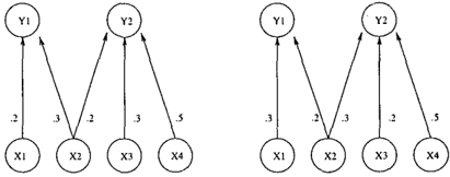
It is not hard to see that if two networks are struc­ turally equivalent, then for any input bias p, they gen­ erate identical distributions on their outputs. We will eventually see that the converse is not true (see Fig­ ure 1), which will complicate the conditions we require on the unknown network.

Given any noisy-OR network, it will prove useful to partition its inputs into sets that we will call basic blocks. Informally, a basic block consists of all those inputs that influence the outputs in an identical man­ ner. Formally, for each input Xi we define the set Ti to contain the (indices of) outputs 1j such that i E Sj (that is, "TJij =f. 1). Thus, Ti consists of just those out­ puts that Xi influences. Then we say that Xi and Xi' are in the same basic block if and only if Ti = Ti', and for every j E Ti, "TJ ij = 1Ji' j. Clearly, the basic blocks define a partition of the input variables.

Now for any basic block B � {XI, ... , Xm} of a noisy­ OR network, there are a number of ways of "naming" or specifying B. One is obviously by the subset of the Xi in B, which allows for the possibility of 2 m distinct basic block names. The following simple lemma shows that for limited fan-in networks, there is a much more succinct way of specifying the basic blocks.

Lemma 3.1 {[K94}) Let N be a noisy-OR network on inputs XI, ... ,Xm and outputs YI, ... , Yn, and let the fan-in of N be bounded by k . For any j, let Sj be the set of inputs connected to output 1j, as defined above. Then any basic block B of inputs is equal to the intersection of k of the Sj and their complements that is, there exists ii, . . . , j k such that

To see this, first note that a basic block B is sim­ ply a collection of inputs, each of which is connected to exactly the same set of outputs. Without loss of generality, let the outputs that B is connected to be

Y1 , . .. , Yr. Then we clearly have

In particular, B is contained in 51. If B = S1, we are finished. Otherwise, by Equation (3), we must be able to choose one of 5 2 , ... , Sr, S r+l, . . . , Sn, and by intersecting with sl, reduce the remaining set size by at least 1 while getting "closer" to B. But since 51 has only k elements to begin with, after only k -1 inter­ sections of the n given in Equation (3), the resulting intersection will be equal to B.

3.2 An Incremental Algorithm Using SEQ's

Armed with the notion of basic blocks, we can now de­ scribe our algorithms at a high level. First we make the behavior of SEQ's more precise. The input to an SEQ consists of a two-layer noisy-OR network, complete with weights, defined on all the inputs X1, . .. , X m and on just a subset Y of the outputs Y1, . .. , Yn. The SEQ returns YES if the input network is structurally equiv­ alent to the subnetwork induced by the target network on Y. Otherwise, the SEQ returns NO.

For now, we simply assume that we have access to SEQ's, and describe an algorithm for exactly recover­ ing the structure of the unknown target network. As we have already mentioned, however, we will eventu­ ally show various conditions under which it is possible to implement SEQ's given only access to samples from the target output distribution. Since the complexity of this implementation will depend crucially on the size of the subnetworks on which the SEQ's are made, we here give an algorithm that only makes SEQ's on small networks.

Let us here reintroduce the assumptions on the target network that we will exploit -namely, that the target network has identical (and known) input biases p, fan­ in bounded by k and at most£ weight values, which we also assume are known. (In order to successfully im­ plement SEQ's, we will later examine some additional restrictions on the parameters, but these will suffice for now.) Under these conditions, there is a simple in­ cremental algorithm for exactly recovering the target network from SEQ's that we will use as our starting point, and then modify.

The simple incremental algorithm proceeds as follows: assuming for induction that the target network re­ stricted to just the outputs Y1, . . . , 1J-1 (that is, the network between all of the inputs X1, . . . , X m and just these first j -1 outputs) has been perfectly recon­ structed, the algorithm proceeds to "add" the struc­ ture on 1j. There are at most n k choices for the set S · J

of inputs connected to 1j; for each such choice, there are at most £k choices for the weights on these connec­ tions. For each of the resulting nk £k ways of "wiring" 1j into the network reconstructed so far, we can then make an SEQ on the entire proposed network on the inputs and Y1, . . . , Yj. Clearly one of the queries will return YES, indicating that the structure is correct, and we can proceed to the next output.

This incremental algorithm would make on the order of n(nk £k) SEQ's, each on a network with as many as n outputs. The size of such queries would result, as we will see in the next section, in a final implementation that required time exponential in n in order to recon­ struct the network from sample data. We now describe an improved algorithm that makes SEQ's whose size depends only on k.

Suppose we have reconstructed the network through Y1, ... , Yj-1, and we divide them inputs into the basic blocks defined by these j -1 outputs. Clearly, in order to decide how 1j should be wired, it suffices to know for every basic block B how many inputs are in B n S j we already know that every input in B is identically connected to the outputs Y1, ... , 1J-1, so we simply need to know how many of these are connected to Y. (and of course, with what weight), and how many ar � not. Notice that the introduction of 1j is naturally "breaking" each previous basic block into at most £ + 1 new basic blocks, according to the connectivity to }j, and the appropriate weight value.

Now the important point is that by Lemma 3.1, if Yj breaks one of the current basic blocks B into two or more new basic blocks, it must already do so in the subnetwork induced by the k outputs comprising the succinct "name" of B. More precisely, in order to de­ termine the connectivity from the basic block B to th � output 1j, we can proceed as follows: take the k out­ puts Yj11 . .. , }jk from Y1, . .. , 1J-1 yielding Equation (2) for B, and look at the subnetwork induced by these k outputs - this will consist of these k outputs, their inputs (of which there are at most k2) , and the connec­ tions between them. We now consider all possible ways of adding the new output 1j to this subnetwork- that is, all possible ways of choosing up to k inputs to 1j from among the k2 inputs of 1j,, . . . , }jk, with the re­ maining inputs to Yj being "new" inputs. For each such . choice (of which there are are most (k2)k = k2k), we will make an SEQ on the resulting subnetwork, and one of them must return YES. For this choice, we can see how many inputs in B are connected to Y. and J, then go on to the next basic block. Note that the suc­ cessful SEQ apparently gives much more information than how many inputs in B should connect to Y. -. 1 J 1 t may a so suggest connectivity to Yj for many of the

other inputs in the subnetwork. However, it is only for the basic block B that connectivity in the subnetwork implies connectivity in the overall network, since this was how we chose the induced subnetwork.

Thus, the for each basic block and each output, we need at most k 2 k£k SEQ's, each on a network with at most k + 1 outputs; since there are n outputs and at most m basic blocks, we obtain:

Theorem 3.2 For any class of fan-in k, identical in­ put bias, two-layer noisy-OR networks with at most e weight values, there is an algorithm for learning a network that is structurally equivalent to an unknown target network from the class with m inputs and n out­ puts using at most mnk2k£k SEQ's, each on a network with m inputs and k + 1 outputs.

The important observations at this point are that the number of queries required is exponential in k, but only polynomial in m and n, despite the fact that the number of networks in the classes considered is expo­ nential in m and n; and that the required SEQ's are on small sets of outputs.

4 Implementing SEQ's from Data

In order to implement an oracle for SEQ's given only sample data from the outputs of the target network, we will take an obvious approach: given a query on a network with outputs Yit, ... , Yir, we will sample the target network distribution restricted to these out­ puts. If the observed distribution on these outputs differs "significantly" from that defined by the query network, we declare the query incorrect and return NO, and otherwise we declare the query correct and return YES. Thus, in order to implement SEQ's, we will need that (sub)networks that are not structurally equiva­ lent generate different distributions, and furthermore that the difference would be noticeable from a small sample.

For the noisy-OR networks we examine, it turns out to be most convenient to express the distribution on the outputs as a set of polynomials over the uniform input bias p; this polynomial is defined by the network structure and weights. As long as networks that are not structurally equivalent give rise to non-identical sets of polynomials, we will be able to argue that we can distinguish different networks on the basis of sam­ ple data, and thus implement the desired SEQ's.

4.1 Polynomials for Noisy-Or Distributions

Consider a noisy-OR network with r output units Y = {Y1, . . · , Yr} and identical input biases p. We would like to compute the probability that the outputs in Y are all 0 simultaneously. Recall that each input Xi is connected to the outputs in Ti. Using the notation of Equation (1), in order for all the outputs in Y be 0, we need that for any input Xi that is set to 1 and is connected to an output }j E Y, Rij = 0. For a given Xi, the probability of this event is rrjETinY 1Jij. Since each input Xi has probability p of being 0 and 1 p of being 1, we have

For a fixed noisy-OR network with outputs Y, we will use Qy(p) to denote the polynomial of Equation (4). Thus, we view the network weights 1Ji j as fixed, with the input bias pas the argument.

Let C be a class of (possibly restricted) noisy-OR net­ works. We say that C has unique polynomials if for any N1 and N2 in C that are not structurally equiva­ lent, there is a set Y of outputs such that QVp) and Q� (p) are not identical (that is, there exists a p such that QVp) =/= Q�(p)), where Q�(p) is the polynomial given by Equation ( 4) for the network N i .

Note that if two distributions agree exactly on the probability that any subset of the outputs is simulta­ neously 0, then the distributions are in fact identical. Thus, if class C does not have unique polynomials, then there are two structurally inequivalent networks in C that generate identical output distributions, and we could never hope to implement SEQ's for this class, or more generally, to exactly learn the structure from observed data. On the other hand, if C does have unique polynomials, we still have work to do, since this only guarantees that for some set of the outputs, and for some value of the input bias p, there is a non-zero difference between the probability of all O's. The first problem - that we don't know which set of outputs yields the differing polynomials - we have essentially already solved, since we have shown how to limit our attention to only k+ 1 outputs at a time in the required SEQ's. The latter two problems - that we only have a guarantee of a difference for some value of p, and that this difference may be too small are tackled in the next section. For now, we simply show several restricted classes of noisy-OR networks with unique polynomials.

We start with the class of noisy-OR networks with just

one weight value.

Lemma 4.1 The class of noisy�OR networks with one weight value has unique polynomials.

This simple example already includes networks of stan­ dard logical OR gates, in which the allowed weight value is 0. Unfortunately, it is possible to show that this lemma cannot be generalized to allow even three weight values - that is, there exist two (rather small) noisy-OR networks that are not structurally equiva­ lent, yet generate identical output distributions (see Figure 1 ). However, in the full paper, we will demon­ strate several other restrictions on noisy-OR networks that do yield classes with unique polynomials. One ex­ ample is the class of networks in which each output }j is associated with just a single weight value TJj -thus, if Xi is connected to }j, then "lii = "li. A similar con­ dition associating each input with just a single weight value also yields unique polynomials. Another suffi­ cient condition is that every weight "li j is one of two fixed values ry or �. with only k inputs to each output having weight ry. This permits networks in which every input influences each output, but with most influences being "weak" (details omitted).

The important points are that the condition of unique polynomials is required in order meet the strong learn­ ing criterion we are aiming for, and that this condition is met for certain natural restrictions on the networks, but certainly not all. For those classes with unique polynomials, the next section provides rather general methods for implementing SEQ's.

4.2 SEQ's from Unique Polynomials

Let us briefly review where we are. We first gave an algorithm assuming SEQ's that learned a network structurally equivalent to the unknown target network, and made SEQ's on subnetworks with only k + 1 out­ puts. We then introduced the notion of a class of net­ works having unique polynomials, argued that it was required in order to meet our learning criterion from sample data, and demonstrated some classes having unique polynomials. In this section, we show that if a class has unique polynomials, then we can in fact implement SEQ's for "most" values of the input bias p.

We first state a general result about polynomials.

Theorem 4.2 Let Q 1 ( p ), . . . , Qr(P) be univariate polynomials, each with degree at most d and leading coefficient at least c. Then for any a, the number of distinct values of p E [0, 1] for which there exists an i satisfying Qi(P) =a is at most dr, and the measure of the set {p: 3iiQi(P)I :Sa} is at most 8dr(al2c) 1 1d .

We omit the proof of this theorem, but it relies on some classical results in approximation theory [R69]. We now show how this result can be used to implement SEQ's from sample data for restricted classes of noisy­ OR networks.

Let C be a class of noisy-OR networks with unique polynomials, and let p E [0, 1]. We say that p is a­ good for C if for any two networks N1 , N2 E C that are not structurally equivalent, there is a subset Y of the outputs such that

In other words, a "good" bias is one that ensures that any two non-equivalent structures have significantly different output distributions.

The following result states that "most" values of the bias p are "reasonably" good for classes of networks with unique polynomials.

Theorem 4.3 Let C be a class of noisy-OR networks with fan-in k and£ weight values multiplying (3. Su p­ pose that C has unique polynomials. Then the measure of p E [0, 1] that are a-good for C is at least 10, for a value of a that is polynomial in 1 I kk4, 1 I £k4, 1 I (3k 3 , and1lcSk2·

Proof : (Sketch ) Since C has unique polynomials, for any networks N i and Ni in C we know that there

exists a set Y of their outputs such that the polyno­ mials Q V p) and Q V p) are not identical. Further­ more, by the basic block arguments already given, we may assume that IYI ::; k + 1. This implies that ni/CP) = Q V p)- Q � (p) t. o. If in addition, ror a given value of p , IR �/( p)j > o:, this pis good for this N i and Ni; if this holds for any Ni and Ni in the class C, we conclude that this pis o:-good for C. The proof proceeds by applying Theorem 4.2 to the set of all n�i (p), with bound on the number of such polynomi­ als derived from the restrictions on the weight values. 0

Thus, provided C has unique polynomials, we can im­ plement SEQ's from observed output data for "most" (but not all) values of the input bias. Provided pis a­ good, we can answer (with high probability) any SEQ by simply sampling sufficiently to determine if there is some subset of the outputs on which the distribu­ tion defined by the queried subnetwork differs from the target distribution by more than o:.

4.3 Wrapping Things Up

The combination of results from the previous sections finally yields the following.

• For the restricted classes of noisy-OR networks discussed in Section 4.1, we have algorithms that will, with probability 1 -o, derive from a suffi­ ciently large random sample of output values a network that is structurally equivalent to the tar­ get network, for "most" values of the input bias.
• The algorithms all reconstruct the target network incrementally, always deciding how to add a new output through a series of SEQ's defined by the current basic blocks. (Section 3.2)
• The SEQ's are implemented by sampling suffi­ ciently from the target output distribution to see if the queried subnetwork generates a distribu­ tion sufficiently similar to assert structural equiv­ alence. (Section 4; Theorem 4.3)
• The probability 1 -o of success by the algorithms is taken over the draw of the random sample. The running time and sample size required by the al­ gorithms will depend only polynomially on the number of outputs of the target network, but ex­ ponentially on the fan-in.
• The measure of the set of input biases for which the algorithms succeed can be made arbitrarily close to 1 at the expense of increased running time. (Theorem 4.3)

More formally, we can establish the following theo­ rem. Similar results can be stated for the other classes of noisy-OR networks that have unique polynomials, discussed in Section 4.1.

Theorem 4.4 Let C be the class of noisy-OR net­ works with one weight value 'T} and fan-in k. There exists an algorithm A, such that for any N E C, and for the input bias p chosen at uniformly in (0, 1], the algorithm A, given p and 'TJ as input, and given access to random examples generated according to the output distribution Np, produces a network N', such that with probability 1 -o the networks N and N' are struc­ turally equivalent. (Here the probability is both over the choice of p and the random sample.) Furthermore, the running time of A is polynomial in m (the number of inputs of N ), n (the number of outputs of N}, 1/ o (the confidence}, 1/((1'T})'T}) (the weight value), and 1/p (the input bias), and exponential in k (the fan-in bound). (More precisely, the running time is bounded by m n (1 /P'T} ) k c , for some constant c.)

Acknowledgements

1. Mansour was supported in part by a grant from the Israel Science Foundation.

References

• (F98] Nir Friedman. The Bayesian Structural EM Al­ gorithm. These proceedings.
• [H96] David Heckerman. A Tutorial on Learning with Bayesian Networks. Microsoft Research Tech­ nical Report MSR-TR-95-06. Revised version, November 1996.
• (K94] M. Kearns, Y. Mansour, R. Rubinfeld, D. Ron, R. Schapire, and L. Sellie. On the Learnability of Discrete Distributions. Proceedings of the 26th Annual ACM Symposium on the Theory of Computing, ACM Press, pp. 273-282, 1994.
• (P95] Judea Pearl. Probabilistic Reasoning in Intelli­ gent Systems: Networks of Plausible Inference. Morgan Kaufmann, 1988.
• [P88] Judea Pearl. Causal Diagrams for Empirical Re­ search. Biometrika 82:669-710, 1995.
• [S93] P. Spirtes, C. Glymour, R. Scheines. Causation, Prediction, and Search. Springer-Verlag, New York, 1993.
• (R69] Theodore J. Rivlin. An Introduction to the Ap­ proximation of Functions. Blaisdell Publishing Company, 1969.