Exploiting Functional Dependence in Bayesian Network Inference

Jifl Vomlel* Department of Computer Science

Aalborg University, Denmark [email protected]

Abstract

In this paper we propose an efficient method for Bayesian network inference in models with functional dependence. We generalize the multiplicative factorization method originally designed by Takikawa and D'Ambrosio (1999) for models with in­ dependence of causal influence. Using a hidden variable, we transform a probability potential into a product of two-dimensional potentials. The multiplicative factorization yields more efficient inference. For exam­ ple, in junction tree propagation it helps to avoid large cliques. In order to keep po­ tentials small, the number of states of the hidden variable should be minimized. We transform this problem into a combinato­ rial problem of minimal base in a particu­ lar space. We present an example of a com­ puterized adaptive test, in which the factor­ ization method is significantly more efficient than previous inference methods.

1 Introduction

The application of Bayesian networks is usually ac­ companied by diverse problems. However, two prob­ lems seem quite common. First, it is often hard to get reliable numerical values of conditional probabilities when there is a large number of parents of a node. Second, in a complex model the exact inference is often infeasible since some probability potentials be­ come too large.

Several authors have realized that in many applica­ tions the first (modeling) problem can be eased by

'Since July 2002 the author is affiliated to the Labora­ tory for Intelligent Systems at the University of Economics, Prague, Czech Republic, e-mail: [email protected]

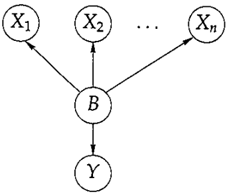
special types of relations between variables, see Hen­ rion (1987), Olesen et a!. (1989). Typical examples are noisy-or, noisy-and, noisy-max, and noisy-min models. They belong to a class of models known as models of independence of causal influence (ICI) or models of causal independence, a concept introduced by Beckerman (1993). Several different definitions of ICI have appeared in literature, see Beckerman and Breese (1994) for a comparison. The most general definition was given by Srinivas (1993) and accord­ ing to this definition ICI can be modeled by use of a Bayesian network with a structure like the one in Fig­ ure 1.

ICI can be exploited in belief updating. One of the earliest examples is the Quickscore algorithm of Beckerman (1989) which exploits noisy-or rela­ tions in the Quick Medical Reference model. Most other approaches are based on a transformation of the network structure. Olesen et a!. (1989) pro­ posed the parent divorcing method. Beckerman and Breese (1994) used a temporal transformation. Zhang and Poole (1996) introduced deputy variables that are used to create a heterogeneous factorization in which the factors can be combined either by multiplication or by a combination operator.

Takikawa and D'Ambrosio (1999) introduced inter­ mediate (hidden) variables to an ICI-model which al­ lowed them to transform an additive factorization of ICI into a multiplicative factorization. The additions are then achieved by standard marginalization of the intermediate variables. Madsen and D'Ambrosio (2000) apply this transformation to the lazy propaga­ tion of Madsen and Jensen (1998) using several inter­ mediate variables for one ICI model. Recently, Dfez (2001) pointed out that the transformation of ICI mod­ els can be done using a single variable.

In Section 2 we generalize the factorization method of Takikawa and D'Ambrosio (1999) so that it applies to any model containing functional dependence. We argue there that, in principle, the factorization by use

of a hidden variable can be applied to any probability potential. In Section 3 we describe how the states of a hidden variable can be found in the case of potentials with functional dependence. In Section 4 we analyse the reduction of the total clique size that the factoriza­ tion method brings and use a computerized adaptive test to show how the factorization method can be ex­ ploited. We present empirical results indicating that the factorization method brings substantial savings in comparison with traditional techniques.

2 Factorization with a hidden variable

We propose a transformation of probability poten­ tials. Our method is a generalization of the method suggested by Takikawa and D'Ambrosio (1999). The transformation is based on the introduction of a hid­ den variable so that a probability potential can be rep­ resented by a product of two-dimensional potentials. In contrast to the usual random variables, states of the hidden variable are not required to be mutually exclusive_!

Let xj, ... I Xn be discrete random variables. The fi­ nite set of values of X;, i = 1, . . . , n will be denoted X; and X = X1 x ... X Xn. Let B be a variable having states from a finite set B.

Definition 1 (Factorization with a hidden variable) Let 1/J be a probability potential defined on X. We say that 1/J can be factorized by use of the hidden variable B if there exist real valued potentials <p1, ... , 'Pn such that for all (x1, ... , X n) E X

Assume a probabilistic model defined as a probabil­ ity distribution P on Xv = X;EvX; and represented as a product of potentials II�=11/J;(xc.), C; � V, where u}=1 C; = V.2 A model obtained through one or more applications of factorization by use of a hidden vari­ able will be referred to as a factorized model.

Evidence on a variable X; is a vector e; with a value equal either zero or one for each state of variable X;. By ec we will denote evidence given on all variables Xc = (Xj)jEc,C � V. We will say that a statexo = (xj)jED of Xo = (Xj)jw,D � V is consistent with an evidence ec if the values of ecnD corresponding to states xcnD are all equal to one. We will write xo �

1 The hidden variable is an auxiliary parameter of a model and need not have any interpretation.

2For example, the sets C;, i = 1, . . . , k can correspond to the nodes in a junction tree representation of a Bayesian network.

ec. The process of computing conditional probability P(xo I e ) for a set D � V and an evidence e is called belief updating, propagation, or probabilistic inference.

Lemma 1 Belief updating performed in a probabilistic model and in corresponding factorized model provide equivalent marginals.

Proof. Inserting an evidence e into a probabilistic model P(xv) means that every potentiall/J;(xe;) is re­ placed by a new potential

For an arbitrary set D � V it holds that

For an arbitrary potentiall/Jj(xc , ), 1 � j � k replaced by its factorized model Lb II£=1 <pe(xe, b), it holds that 1/! j( x c , , e)= m=l <pe(xe, b, e ) . Therefore

The last formula corresponds to computations per­ formed during belief updating in the model with po­ tentiall/Jj replaced by a factorized model. D

Remark. Note that the hidden variable B can be elim­ inated any time, which means that it is left to a belief updating method to decide when B is eliminated. For example, we can let a triangulation algorithm decide in which cliques variable B is included when creating a junction tree.

The lemma allows straightforward application of the factorization method to belief updating methods, where factors are combined by multiplication (e.g. Variable Elimination, Shafer-Shenoy, and Lazy Prop­ agation methods). There is a problem with applica­ tion of the factorization method to belief updating methods that use division for discarding a message passed through a separator in the opposite direction (e.g. Hugin and Lauritzen-Spiegelhalter methods). We allow negative numbers in potentials therefore a potential 1/J( S) = LC\ S 1/J ( C) in a separator S that is computed from a clique potential 1/J( C) may contain a zero due to the combination of positive and neg­ ative values of 1/J( C) (S. Moral and J. Dfez, personal communication).

Factorization with a hidden variable can be applied to any probability potential, no matter whether it is a conditional probability table or a potential created during belief updating. Factorization can be used, for example, to modify Lazy Propagation method of Madsen and Jensen (1998). In lazy propagation the messages consist of lists of potentials which are com­ bined only if necessary. During the propagation, large potentials could be checked as to whether they might be factorized. Similarly, a large probability tree could be replaced by a product of trees in penniless propa­ gation of Cano et a!. (2000). Factorization can be also used to approximate large potentials in an approxi­ mate propagation method.

In this paper, we will not study the factorization of an arbitrary probability potential. We will only deal with the factorization of potentials with functional depen­ dence.

Definition 2 (Functional dependence) Let 1jJ be a probability potential defined on Y X Xt x . . . X Xn, the Cartesian product of sets of states of discrete ran­ dom variables Y, X1, . . · , Xn. We say that Y is func­ tionally dependent on X1, . . . , Xn if there is a function f : X t X ... X Xn r-t Y such that

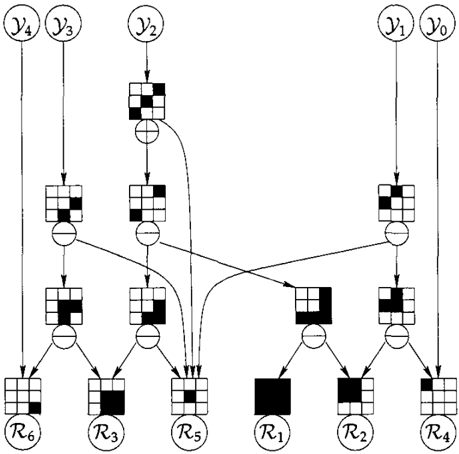
An example of a model containing functional depen­ dence is an ICI model, see Figure 1.

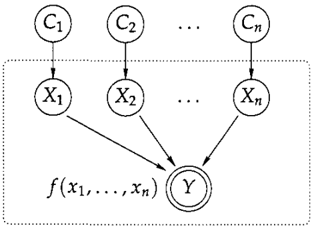
In Figure 2 the factorization with a hidden variable B of the the part with functional dependence of the ICI model of Figure 1 is depicted. Every edge in the undirected graph corresponds to a new potential.

3 States of hidden variables

In this section we will discuss how the states of a hid­ den variable can be found to bring substantial savings

into belief updating. We will utilize two set opera­ tions that are special cases of symmetric difference. LetA, B <;;;X.

Definition 3 (Symmetric difference) Symmetric dif­ ference of A and B is A 'V B= (A\ B) U ( B \A).

Definition 4 (Proper difference) If A 2 BorA <;;; B, then the proper difference of A and B is defined as AeB=A'VB.

Definition 5 (Disjunctive union) Let A, B <;;; X. If An B = 0, then the disjunctive union of A and B is defined as A Ell B =A 'V B .

Rectangular subsets of X = x t = t X; will play a special role in our transformation.

Definition 6 (Hyperrectangle) R is a hyperrectangle iff R = x?=t' 'D;, 0 f= 'D; <;;;X;

We will use expressions expr( Rt, . . . , Rm) consist­ ing of operators e, Ell, and hyperrectangles Ri, j = 1, ... , m. An expression is called legal if operators 8 and Ell are applied according to their definitions. Parentheses are used to express precedence of the op­ erators' application. Every legal expression can be represented as a directed tree having (a) one source node corresponding to the result of the expression, (b) nodes corresponding to operators 8 or Ell, and (c) sinks, one sink for each hyperrectangle Ri used in the expression. Each intermediate node has two operands as its children.

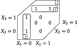
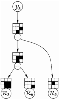
Example 1 (A legal expression) Let X = {0, 1, 2} x { 0, 1, 2} and let three subsets of X be n3 {(1, 1), (1, 2), (2, 1), (2, 2)},

Rs {(1, 1)}, and 三

n6 {(2, 2)} .

Y3 = expr( R3, Rs, R6) = ( R3 e R6) e Rs is a legal expression. It can be represented by the directed tree displayed in Figure 3.

Each subset of X is represented by a pattern in a 3 x 3 grid attached to the corresponding node. A pane in the grid correspond to an element of X. The pane is filled if the set contains the corresponding element. 0

The following two relations will be used to decom­ pose sums over potentials.

Proposition 1 Let A, B, C <::;; X and 1jJ be a potential de­ fined on X.

Recall that we aim at factorizing potentials 1jJ defined on the Cartesian product xl X ... X Xn X y that con­ tain variable Y functionally dependent on X1, ... , Xn by function f : xl X ... X Xn >--> y so that

Next, we will show how such a factorization can be found.

An easy way of obtaining a factorization is to define a set of states B of a hidden variable B so that it contains one state for each element x' of X = X1 x . . . x Xn, i.e. we have a bijection b : X <--> B. The potentials are then defined

Recall that 1/J (y, x') = 1 iffy = f(x'). Therefore func­ tion h(y, b(x')) is an indicator function equal to one if y = f(b-1(b(x'))) and zero otherwise. Function g(x, b(x')) = m=l g;(X;, b(x')) is an indicator function equal to one if x = x' and zero otherwise. Obviously, this factorization does not bring any savings for belief updating. However, we will use it as a starting point to derive a better factorization.

We can rewrite formula 1 as

Definition 2 implies that for every state y e of variable Y there is a set Ye = {x' E X, f(x') = ye} and that if x' E Ye thenh(ye,b(x')) = 1, otherwiseh(ye,b(x')) = 0. Thus, for an arbitrary Y e E Y:

Assume that Ye is equal to the result of a legal expres­ sion e x p r e( n ] , ... 'nm) using the operators 8, E&, and hyperrectangles Rj, j = 1, . . . , m. Then, using Propo­ sition 1 we can rewrite formula 3 as

where expression expr( is constructed from expres­ sion ex pre by the following replacement rules:

Note that there may be multiple occurrences of a hy­ perrectangle Rj in one expression. Let B' be the set of all hyperrectangles Rj in all expressions expre, C = 1, ... , IYI. Since- and+ operators are normal minus and plus operators, we can summarize the occurrence of each hyperrectangle R E B' in expression expre by use of an integer-valued function h'(ye, Rj)· We give an example of the construction of h' (y e, Rj) in Exam­ ple 2. Thus, we can write formula 4 as

Recall that g(x,b(x')) is an indicator function equal to one if x = x' and zero otherwise. Thus, g'(x, R) = Lx'E'R g(x, b(x')) is another indicator function equal to one if x E R. Since R is a hyperrectangle, we can test whether x E R independently for each X;, i = 1, ... , n and write the indicator function as

Finally, we substitute the new indicator function into formula 5:

Formula 6 gives us a new factorization of t/J by use of a hidden variable with one state for each element R of B'. The set of hyperrectangles B' will be called a base.

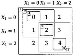
Example2(ADD) Let X= {0,1,2} x {0,1,2} and f (x! , x z ) = x1 + xz. A base of hyperrectangles is

The hyperrectangles can be depicted in a figure:

Relations between Ye, £ = 0, ... , 4 and the base are

They are summarized in the potential h' (Y, B')

y	n,	nz	n,	n4	ns	n6
0	0	0	0	+1	0	0
1	0	+1	0	-1	-1	0
2	+1	-1	-1	0	+2	0
3	0	0	+1	0	-1	-1
4	0	0	0	0	0	+1

The potentials g;(x;, B'), i = 1, 2 are

X;	n,	nz	n,	n4	ns	n6
0	+1	+1	0	+1	0	0
1	+1	+1	+1	0	+1	0
2	+1	0	+1	0	0	+1

0

Example 3 (Boolean function) Let X = {0, 1 p and f be a Boolean function (X1 V X2) => (X2 II X3). This is equivalent to ( ·X1 II ·Xz) V (Xz II X3), from which we can construct a base3

Note that Jo = R3 θ (R2 Φ R1) and Ji = R2 Φ R1.

0

The scope of this paper does not allow more exam­ ples for different functions. At least, we refer to (Dfez 2001) where the factorization of the MAX function is proposed. There is a direct correspondence between Dfez's f1 matrix and our h(Y, B) potential. In this case the number of states of variable B is equal to the num­ ber of states of variable Y since base B contains IYI nested hyperrectangles.

Minimal base of hyperrectangles

The smaller the base, the better factorization. We for­ mally state the task as a combinatorial problem.

Definition 7 (Minimal base of hyperrectangles) For a function f : X >-+ Y, X = x j = 1 X ; find a base B = {R1, ... , R k } of minimal cardinality k such that:

• for j = 1, ... , k : Ri = xj=1D;, 0 =f D; <;;X;, i.e. Ri is a hyperrectangle,
• for every ye E Y the set Ye = {x EX, f(x) = Ye} can be generated from base B using operations of proper difference e and disjunctive union E£).

Theorem 1 Every probab i l i ty potent i al t/J(y, x ) repre­ sent i ng funct i onal dependence y = f ( x ) can be factor i zed by use of a h i dden var i able hav i ng one state for each hyper­ rectangle from a base of hyperrectangles of Juncti on f.

3 It does not generally hold that a base can be directly constructed from the disjunctive normal form. E.g. (X 1 II X2) V (X1 II X3) must be rewritten as (X1 II X2) V (X1 II ·X2 II X3) to make clauses mutually exclusive.

一

Proof. The above considerations show how such factorization can be constructed and thus represent a proof of the theorem. D

The minimal base of hyperrectangles (MBH) problem thus provides a systematic way of minimizing the to­ tal size of new potentials. Recall that each legal ex­ pression can be represented as a directed tree (Fig­ ure 3). Every solution of the MBH problem corre­ sponds to I Y I legal expressions using hyperrectangles from a minimal base B. Therefore, we can represent it as a directed acyclic graph (DAG) having nodes cor­ responding to sets Ye for every ye E Y as its sources and nodes corresponding to hyperrectangles from the base B as its sinks. See Figure 4 where the solution for the ADD function from Example 2 is presented.

The MBH problem can be thus solved by searching a DAG that (a) represents legal expressions (b) for every ye E Y the set Ye corresponds to one source in the DAG and (c) the DAG has minimal number of sinks. We are not aware of any polynomial algo­ rithm providing a solution of the MBH problem in the general case. We conjecture that the MBH problem is NP-hard. We intend to further explore the MBH problem and its siimilarity with problems in multi­ party communication complexity, see Kushilevitz and Nisan (1997).

Nevertheless, in most cases it will be possible to per­ form an extensive search since we are interested in a solution only if the resulting minimal base is rela­ tively small and the original potentials are not very large. Furthermore, for commonly used functions a minimal base can be computed in advance.

The cardinality of the minimal base B is bounded from below by the number of states of variable Y, i.e. IBI 2': I YI. It means, for example, that the cardinality of the minimal base of the ADD function with argu­ ments X; such that X;= {1, .. . ,s} fori= 1, ... ,n is at least IYI = Ii'=1( IX;I -1) = n · (s -1).

4 Evaluation of the factorization method

Reduction of the total clique size

The primary goal of the factorization with a hidden variable is to speed up Bayesian network inference by reducing the total clique size. It is achieved by fac­ torizing deterministic potentials, i. e. potentials rep­ resenting functional dependence of a varible Y on X; fori = 1, ... n. The transformation corresponds to the introduction of one variable B and an arc B _. Y and to the replacements of arcs X; _. Y by B _. X; for i = 1, ... n in each transformed potential.

Next we will compare a junction tree method with and without the use of our transformation for the de­ terministic potentials. Assume we connect one de­ terministic potential to a model. In the standard ap­ proach all nodes X; fori = 1, ... n have to be married (pair-wise connected by edges). In the worst case the triangulation may require all nodes from the original model to be connected to all X;, i = 1, ... n. It in­ creases the total clique size of the junction tree by fac­ tor TI;'=1IX;I = lXI, where X= X1 x ... x Xn. When we use factorization with hidden variable B the trian­ gulation may require that all nodes from the original model to be connected to variable B in the worst case. It increases the total clique size of the junction tree by factor IBI. In this case the total clique size is reduced by the factor rat.

For simplicity, let us assume that all deterministic po­ tentials have the same number of variables, no vari­ able is shared by two or more deterministic poten­ tials, all variables have the same number of states, and all deterministic potentials can be transformed by use of a hidden variable B with the same num­ ber of states. When a second potential is connected to the original model it may require that all nodes from the original model are again connected to all nodes x;, i = 1, ... n in the second potential. It means that the total size of junction tree after connecting r de­ terministic potentials increases by factor I X I r in the standard approach and by factor IBI' when using the factorization with hidden variable B. Thus one can say that the saving is proportional to � = (rat) r.

Often, it will not be necessary to add edges to all nodes in the original model either because they are already there or because the introduction of a deter­ ministic potential creates cycles that do not include all nodes from the original model. Typically, when several deterministic potentials are connected to the model the model gets more and more saturated and the increase of the total size of the junction tree is slower. However, this would affect similarly the stan­ dard approach and the method based on factorization with hidden variable.

We represented clique potentials as tables. If we represented them as lists of factors we would lower space requirements for all three methods. It is pos­ sible to make cliques even smaller by searching sub­ expressions that are repeated in functions of different deterministic potentials.

For an experimental evaluation of the factorization of noisy-max on the CPCS network see (Diez and Galan 2002). We tested performance of the factorization with hidden variable on a model for a computerized adaptive test.

A computerized adaptive test of basic operations with fractions

In this section we show that factorization with a hid­ den variable brings substantial savings for inference in computerized adaptive testing. The objective of computerized adaptive testing (CAT) is to construct an optimal test for each examinee. During the test administration, the examinee's knowledge level is es­ timated and questions appropriate for the estimated level are selected.

Almond and Mislevy (1999) proposed to use graphi­ cal models for CAT. Their model consists of one stu­ dent model and several evidence models, one for each task or question. The student model describes rela­ tions between examinee's skills, abilities, etc. Each evidence model corresponds to an observation (a question or a task). It is often reasonable to assume that an observation T is conditionally independent of other observations and skills, given a collection of skills relevant for observation T.

An evidence model is connected to the student model only if it contains evidence. This helps to keep the actually used model small. However, when several evidence models are connected, cliques in the junc­ tion tree may become too large and the inference may become slow or intractable. If evidence models con­ tain potentials with deterministic dependence the fac­ torization with hidden variables can reduce the total clique size and speed up the inference.

We evaluated the factorization method on a Bayesian network for testing basic operations with fractions. The student model contained 21 nodes represent­ ing skills and misconceptions. The description of the model and its construction process can be found in Vomlel (2002) and Bo.tenas et a!. (2001).

For each task an evidence model was created. An example of a task is � -tz Assume that a student is able to solve certain tasks if and only if she has all necessary skills (SB, CL, ACL, CD , ACD) and does not have any related misconception (MSB) . Then we can describe a task formally by a logical formula Y ¢;> SB & CL & ACL & CD & ACD & -, MSB. The assumption of deterministic relations between skills and the actual outcome of a task is unrealistic. A student can make a mistake even if she has all abil­ ities needed to solve a given task. On the other hand, a correct answer does not necessarily mean that the student has all abilities since she may have guessed the right answer. We model "guessing" using con­ ditional probability P(T I -, Y) and "mistakes" using P( -, y I Y).

We applied the factorization with a hidden vari­ able to potentials in evidence models representing a Boolean function. Each hidden variable had only two states. For example, in the evidence model of task T above the variable B has two states b( Ro) and b( RI), where Ro is the set of all possible configura­ tions of variables SB, CL, ACL, C D , ACD , MSB and R1 = { (1, 1, 1, 1, 1, 0 ) }.

An evidence model is connected to the student model only if it contains evidence. We observed how the total size of potentials in the resulting model grows with more evidence models being connected to the student model. Three methods were compared: (1) evidence models where a task is a child of all nodes in its footprint, (2) hierarchical evidence models cor­ responding to the result of transformation by the par­ ent divorcing method Olesen et a!. (1989), and (3) ev­ idence models factorized by use of a hidden variable.

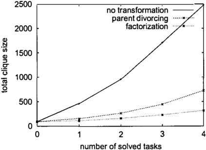
Table 1: Average total clique size.

number of solved tasks

transformation	0	1	2	3	4
none	92	467	961	1709	2408
parent divorcing	92	157	268	449	728
factorization	92	114	163	232	320

Table 1 and Figure 5 asummarize the results. Pro­ vided numbers are the average of the total clique size for all possible orderings of tasks. Observe that fac­ torization results in significantly smaller cliques.

R 6

Acknowledgments

I would like to thank Claus Skaanning for inspiring me to work on the task of efficient inference in CAT. I am grateful to Milan Studeny, Jiff Matousek, and Jiff Sgall for their comments on the MBH problem, An­ ders L. Madsen for his assistance with Hugin, Kirsten Bangs0 Jensen for organizing the paper tests of frac­ tions in Bmnderselev High School, Regitze Larsen for suggestions that improved the readability of the text, and the Decision Support Systems group at Aalborg University for the inspiring, friendly working envi­ ronment. This paper also benefited from the com­ ments of anonymous reviewers and Francisco J. Dfez. I was supported by the Grant Agency of the Czech Republic through grant nr. 201/02/1269.

References

Almond, R. G. and R. J. Mislevy (1999). Graphical models and computerized adaptive testing. Ap­ plied Psychological Measurement 23 (3 ), 223-237.

Butenas, L., A. Brilingaite, A. Civilis, X. Yin, and N. Zokaite (2001). Computerized adaptive test based on Bayesian network for basic operations with fractions. Student project report, Aalborg University. http: I /www. cs. auc. dk/library.

Cano, A., S. Moral, and A. Salmer6n (2000). Penni­ less propagation in join trees. International Jour­ nal of Intelligent Systems 15 , 1027-1059.

Dfez, F. (2001). Efficient computation for the Noisy MAX. In Aetas de Ia IX Conferencia de Ia Aso­ ciaci6n Espanola para Ia Inteligencia Artificial (CAEPIA 2001), Gij6n, Espana, pp. 1115-1124.

Dfez, F. J. and S. F. Galan (2002). An efficient factor­ ization for the noisy MAX. International Journal of Intelligent Systems. Accepted for publication.

Beckerman, D. (1989). A tractable inference al­ gorithm for diagnosing multiple diseases. In M. Henrion, R. D. Shachter, L. N. Kana!, andJ. F. Lemmer (Eds.), Proc. of the Fifth Annual Conf on Uncertainty in AI, pp. 163-171.

Beckerman, D. (1993). Causal independence for knowledge acquisition and inference. In D. Beckerman and A. Mamdani (Eds.), Proc. of the Ninth Conf on Uncertainty in AI, pp. 122-127.

Beckerman, D. and J. S. Breese (1994). A new look at causal independence. In R. L. de Mantaras and D. Poole (Eds.), Proc. of the Tenth Conf on Uncertainty in AI, pp. 286-292.

Henrion, M. (1987). Some practical issues in con­ structing belief networks. In L. N. Kana!, T. S. Levitt, and J. F. Lemmer (Eds.), Proc. of the T hird Conf on Uncertainty in AI, pp. 161-174.

Kushilevitz, E. and N. Nisan (1997). Communication Complexity. Cambridge University Press.

Madsen, A. L. and B. D'Ambrosio (2000). A factor­ ized representation of Independence of Causal Influence and Lazy Propagation. International Journal of Uncertainty, Fuzziness and Knowledge­ Based Systems 8(2), 151-165.

Madsen, A. L. and F. V. Jensen (1998). Lazy prop­ agation in junction trees. In G. F. Cooper and S. Moral (Eds.), Proc. of the Fourteenth Conf on Uncertainty in AI, pp. 362-369.

Olesen, K. G., U. Kjrerulff, F. Jensen, F. V. Jensen, B. Falck, S. Andreassen, and S. K. Andersen (1989). A MUNIN network for the median nerve-a case study on loops. Applied Artificial Intelligence 3, 384-403. Special issue: Towards Causal AI Models in Practice.

Srinivas, S. (1993). A generalization of the Noisy­ Or model. In D. Beckerman and A. Mamdani (Eds.), Proc. of the Ninth Conf on Uncertainty in AI, pp. 208-215.

Takikawa, M. and B. D'Ambrosio (1999). Multi­ plicative factorization of noisy-max. In K. B. Laskey and H. Prade (Eds.), Proc. of the Fifteenth Conf on Uncertainty in AI, pp. 622--{;30.

Vomlel, J. (2002). Bayesian networks in educational testing. Manuscript in preparation.

Zhang, N. L. and D. Poole (1996). Exploiting causal independence in Bayesian network inference. Journal of Artificial Intelligence Research 5, 301328.