Exploiting the Rule Structure for Decision Making within the Independent Choice Logic

David Poole*

Department of Computer Science University of British Columbia

Vancouver, B.C., Canada V6T 1Z4

[email protected] http://www.cs.ubc.ca/spider/poole

Abstract

This paper introduces the independent choice logic, and in particular the "single agent with na­ ture" instance of the independent choice logic, namely I CLoT . This is a logical framework for decision making uncertainty that extends both logic programming and stochastic models such as influence diagrams. This paper shows how the representation of a decision problem within the independent choice logic can be exploited to cut down the combinatorics of dynamic program­ ming. One of the main problems with influence diagram evaluation techniques is the need to opti­ mise a decision for all values of the 'parents' of a decision variable. In this paper we show how the rule based nature of the ICLoT can be exploited so that we only make distinctions in the values of the information available for a decision that will make a difference to utility.

1 Introduction

Most current approaches to solving decision problems un­ der uncertainty involve a case analysis on all available in­ formation (for example on all current and past observations and past actions in influence diagrams [Howard and Math­ eson, 1981; Cooper, 1988; Shachter and Peot, 1992; Qi and Poole, 1995], or on the current belief state in partially ob­ servable Markov decision problems (PO MOPs) [Monahan, 1982; Cassandra et al., 1994]).

In this paper, we consider how a logic-based representation of decision problems that treats causal rules as logic pro­ grams can be exploited to reduce the case analysis for dy­ namic programming. This representation that allows one to express logical rules and choices made by various agents, is capable of representing general decision problems (that ex­ tends both influence diagrams and (finite stage) POMDPs).

•

Scholar, Canadian Institute for Advanced Research

The logic is the independent choice logic (ICL) that allows for a space of independent choices and a logic program that gives the consequences of these choices. The choices can be made by nature (which has probabilities over the choices) or by purposive agents (who are trying to max­ imise their utility). The ICL extends the author's probabilis­ tic Hom abduction [Poole, 1993b] to include negation as failure and multiple agents. In this paper we only consider the decision theoretic (single agent under uncertainty) case. For the no-agent case (with probabilities over choices), the rules induce an independence equivalent to that of Bayesian networks. The rules also allow the representation of a form of 'propositional independence' where one variable may only be dependent on another for some values of a third variable. It is this last property that we exploit in this pa­ per.

The main point of this paper is to show how the rule­ structure can be exploited to gain efficiency. The rules pro­ vide a modular specification of utility, and a modular spec­ ification of what will be observed when a decision is made (this is similar to using decision trees to specify the proba­ bility and utility tables [Smith et al., 1993; Boutilier et al., 1995]). Instead of optimizing a decision for each of its in­ formation states, we 'mesh' the decision trees for the 'ob­ servables' (the information available when the decision is made) and the decision trees for the utilities, and only make the distinctio n s in the observables that matter (would lead to different utilities). We show by example that this can cut down on the number of optimizations that we need to do. The meshing becomes complicated when interleaved with dominance testing-we want to prune dominated de­ cisions as soon as possible, so we don't make distinctions that are only important for decisions than can be shown to be non-optimal.

This paper could have been described in terms of decision trees (as does [Boutilier et al., 1995] using a similar idea for fully observable MOPs, see Section 6). This was not done for a number of reasons. The ICL forms a simple log­ ical framework that includes influence diagrams (the rules can encode all of the dependencies of an influence diagram

• -we don't need the influence diagram and the rules), as well as being interesting in its own right as a mix of logic and decision/game theory [Poole, 1995b]. The meshing is also easily described in this framework in terms of 'expla­ nations'. The ICL also naturally has a way to include log­ ical variables, and thus we allow for p arame trizable influ­ ence diagrams (see [Poole, 1993b] for a description of the purely probabilistic case).

2 The Independent Choice Logic

The Independent Choice Logic specifies a way to build possible worlds. Possible worlds are built from choosing propositions from independent alternatives, and then ex­ tending these 'total choices' with a logic program. This sec­ tion defines the single agent case ICLoT .

There are two languages we will use: £F which, for this paper, is the language of acyclic logic programs [Apt and Bezem, 1991 ], and the language £Q of queries which we take to be arbitrary propositional formulae (the atoms cor­ responding to ground atomic formulae of the language£ F). We write I f--q where I E £p and q E £q if q is true in the unique stable model of I or, equivalently, if q follows from Clark's completion of q (the uniqueness of the stable model and the equivalence for acyclic programs are proved in [Apt and Bezem, 1991]). See [Poole, 1995a] for a de­ tailed analysis of negation as failure in this framework, and for an abductive characterisation of the logic.

Definition 2.1 A choice space is a set of sets of ground atomic formulae, such that if C1, and C2 are in the�choice space, and Ct ::1 C2 then Ct n C2 = {}. An element of a choice space is called a choice alternative (or sometimes just an alternative). An element of a choice alternative is called an atomic choice. An atomic choice can appear in at most one alternative. 1

Definition 2.2 An ICLoT theory is a tuple (Co,C�,0,1l',Po,.1") where

• Co called nature's choice space, is the choice space of al­ ternatives controlled by nature.
• Ct called the agent's choice space, is the choice space of alternatives controlled by our agent (what the agent de­ cides to do). No atomic choice can be both in an ele-

1 Alternatives correspond to 'variables' in decision theory. This terminology is not used here in order to not confuse logical variables (that are allowed as part of the logic program), and ran­ dom variables. An atomic choice corresponds to an assignment of a value to a variable; the above definition just treats a variable hav­ ing a particular value as a proposition (not imposing any particu­ lar syntax); the syntactic restrictions and the semantic construction ensure that the values of a variable are mutually exclusive and cov­ ering, as well as that the variables are unconditionally independent (see [Poole, 1993b])

• ment of Co and in an element of C1 (i.e., VC o E Co VCt E Ct Co n Ct = {}). LetC =Co U Ct.
• 0 the observables is a set of sets of ground atomic formu­ lae. Elements of 0 are called observation alterna­ tives; elements of observation alternatives are called atomic observations. N.B. elements of observation alternatives can unify with the head of rules or can be elements of choice alternatives.
• 1r the observable function, is a function 1r : C 1 -? 2°. The idea is that when the agent decides which ele­ ment of A E Ct to choose, it will have 'observed' one atomic observation from each observation alterna­ tive in 1r{A). Elements of 1r ( A ) are the information available to the agent when it has to choose an element of A. We assume a 'no forgetting' constraint 2 which means that the element of C 1 are totally ordered and if Ct < C2 then Ct E 1r{C2) and 1r(Ct) c 1r{C2).
• Po is a function UCo -? [0, 1) such that VC E C0, Ecec Po(c) = 1. I.e., Po is a probability measure over the alternatives controlled by nature.
• .1" called the facts, is an acyclic logic program such that no atomic choice (in an element of C) unifies with the head of any rule, and such that there is an acyclic or­ dering [Apt and Bezem, 1991] where every element of every element of 1r(A) is before every element of A.

The independent choice logic specifies a particular seman­ tic construction. The semantics is defined in terms of pos­ sible worlds. There is a possible world for each selection of one element from each alternative. What follows from these atoms together with .1" are true in this possible world.

Definition 2.3 If S is a set of sets, a selector function on S is a mapping r : S -? US such that r( S) E S for all S E S. The range of selector function r, written 'R( r) is the set { r{S): S E S}.

Definition2.4 Given ICLoT theory (Co,C�,0,1l'�P0,.1"), let C = Co U Ct. For each selector function r on C there is a possible world wr. If I is a formula in language £Q. and wr is a possible world, we write Wr F= I (read I is true in possible world Wr ) if .1" U 'R( T ) f-. I.

The existence and uniqueness of the model follows from the acyclicity of the logic program [Apt and Bezem, 1991].

Definition 2.5 If S is a set of sets, the expansion of S, writ­ ten expansion(S) is the set {'R( r)lr is a selector function onS}.

2 This constraint can be weakened slightly when the utility can be decomposed into sums [Zhang et al., 1994)

The expansion of S corresponds to the cross product of the elements of S and, when S consists of non-intersecting sets, to the set of minimal hitting sets [Reiter, 1987] of S. The set of possible worlds corresponds to the expansion of C.

Definition 2.6 An ICLoT theory is utility complete if for each possible world w.,. there is a unique number u such that w.,. I= utility( u ). The logic program will have rules for utility( u ).

Definition 2. 7 An I CLoT theory is observation inconsis­ tent if there exists possible world w.,., and there exists 0 E 0 with Ot E 0, 02 E 0, Ot "' 02 SUCh that w.,. F Ot A 02. Otherwise the I CLoT theory is observation consistent. An ICLoT theory is observation complete if for all possible worlds w.,., and for all 0 E 0, there exists o E 0 such thatw.,.l= o.

The above definitions are to make sure that we can treat the elements of 0 as random variables. Unlike elements of C, they are not exclusive and covering 'by definition'. We will always require a theory to be observation consistent, but, when we have negation as failure in the logic [Poole, 1995a] we will not require the theory to be observation complete (there may be an extra, unnamed element of each element of 0). Note that observation consistency is not a severe re­ striction - we can always make 0 a set of singleton sets, but then we can't exploit the exclusiveness of observations.

In this paper we assume all our theories are observation con­ sistent and complete.

If an ICLoT theory is observation consistent and observa­ tion complete, then for each world w.,. there is a unique el­ ement of expansion( 0) that is true in w.,.. Also, for each C E C1 there is a unique element of expansion( 1r ( C)) that is true in w.,., this element is written here as 1r.,. ( C).

Definition2.8 If(Co,Ct,0,1l',Po,F) is aniCLoT theory, then a (pure) strategy is a function u on C1 such that if C E C1, u( C) is a function expansion( 1r ( C)) -+ C.

The elements of expansion( 1r ( C)) are the information available when the decision C is made. In other words a strategy specifies which element of C (for each C E C1) to choose ('do') for each of the possible observations.

Definition2.9 If ICLoT theory (Co,Ct,0,1l',Po,F) is utility complete, and u is a strategy, then the expected util­ ity of strategy u is

(summing over all selector functions r on C = Co U Ct) where

(this is well defined as the theory is utility complete), and

u(r) is the utility of world w.,.. p(u,r) is the probability of world r under strategy u. For the worlds that could be the result of what the agent chooses (i.e., when the selection function r selects the same element of A as does the strategy u ), the probability is the product of the independent choices of nature. It is easy to show that this induces a probability measure (i.e., for each strategy, the sum of the probabilities of the worlds is 1).

2.1 Representing an inftuence diagram

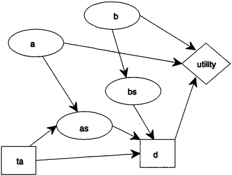
In this section we axiomatise the influence diagram of Fig­ ure 1 in order to demonstrate how the above semantic framework can represent decision problems. This example will also be used to demonstrate our algorithm. In this dia­ gram there is a noisy sensor forb, namely bs, and a control­ lable sensor for a, namely as (the agent can control which aspect of a it senses).

The problem be represented in our framework as:

C1 = {{ta(hi), ta(low)}, {d(O), d(l), d(2)}}. There are two decisions to be made: the agent must choose one of two possible values for ta and one of three possible values for d.

The agent has no information available when choosing a value for ta.

When choosing a value for d the agent will know values for ta, as and bs.

Co= {{a(low),a(med),a(hi)}, {b(pos),b(neg)}, {false..pos, true_neg}, {false_neg, true..pos} }. a can have one of three values, b one of two values, the other two alternatives specify the noise of the bs sensor.

Within the facts, we axiomatise how the 'sensors' work. bs is a noisy sensor of b:

We can specify the reliability of the sensor as:

as is a sensor which we can control as to whether it detects the high values for a or the low values for a (depending on the value of ta ):

as( neg)+-ta(lo) /1. a( hi)

We specify the priors on a and b as:

Finally the rules specify the utility function.

utility(4) +-d(O) utility(lO) +-a( hi) /1. d(l) utility(3) +-a(med) /1. d{l) utility(O) +-a(lo) /1. d(l) utility(2) +-a( hi) /1. b{pos) A d(2) utility(5) +-a( med) /1. b{pos) /1. d(2) utility(9) +-a(lo) /1. b(pos) /1. d{2) utility( B) +-b(neg) /1. d(2)

The above represents the whole decision problem.

Note that the rules for utility and for the probability of as incorporate much more structure than is reflected in the in­ fluence diagram.

3 Sowhat?

We have presented what seems like quite a complicated se­ mantic construction. The main question arises is "So what; why should anyone be interested?"

First of all this is a language that forms a bridge between the purely logical languages, and the probabilistic and decision theory representations.

If Co is empty, this is a representation for classical planning that allows for concurrent actions, and uses action comple­ tion (in a similar way to how [Reiter, 1991] solves the frame , problem). We can axiomatise the world using logic pro­ grams. We have, however, a more sophisticated way of han­ dling uncertainty than just disjunction.

Bayesian networks [Pearl, 1988] can be modelled by Co and :F, in the same way that probabilistic Hom abduction [Poole, 1993b] models Bayesian networks. What is added is a richer language for :F, with negation as failure and fewer restrictions on the form of the rules [Poole, 1995a], as well as agents with goals [Poole, 1995bl

The language is closely related to influence diagrams [Howard and Matheson, 1981]. Elements of C1 correspond to decision nodes in influence diagrams, with 1r(A) corre­ sponding to the 'parents' of the decision node (these rep­ resent information availability when making the decision). The value node is represented as the rules (in :F) that imply utility( u) for some u.

The main problem considered in this paper is how the rep­ resentation can be exploited for computational gain.

Influence diagram evaluation procedures can be divided into two classes:

1. Those that do dynamic programming, optimizing the last action first [Shachter, 1986; Cooper, 1988;
2. Shachter and Peot, 1992; Zhang et al., 1994].
3. Those that convert the influence diagram into a deci­ sion tree (e.g., [Howard and Matheson, 1981; Qi and Poole, 1995]), and search it using a search method such as *-minimax [Ballard, 1983].

Once it has been realised that efficient Bayesian network al­ gorithms can be used for the probabilistic part of the rea­ soning [Cooper, 1988; Qi and Poole, 1995], the maiD cost is in the number of optimizations that needs to be done. For each of the values of the parents of a decision node, one op­ timization is done. This can be improved in the decision tree methods by not considering those assignments to par­ ents that will have zero probability [Qi and Poole, 1995], but there is still much more that can be done.

The main claim of this paper is that we can exploit the rule­ based structure to gain efficiency. We show how the rule

structure can be exploited to reduce the number of opti­ mizations (the technique reported here is orthogonal to the idea of removing of impossible conditioning scenarios, so in principle both could be used).

4 Abductive characterisation

The structure is exploited by the use of 'explanations'. In­ stead of reasoning in the space of possible worlds (or in the space of expansion( 1r ( C))), we reason in the space of ex­ planations. These explanations only make the distinctions needed.

In this section we present the 'abductive' view for the case without negation as failure in the language. There are some interesting issues [Poole, 1995a] that arise in combining this with negation as failure, but these will only complicate this paper.

Definition 4.1 A set "' of atomic choices is consistent if there is no alternative A E C such that l A n "'I > 1.

Definition 4.2 A composite choice on JC � C is a set con­ sisting of exactly one element (atomic choice) from each C E /C.

Definition 4.3 An explanation of ground formula g i s a composite choice"' on a subset of C such that FU"' F= g. A covering set of explanations of g is a set of explanations of g such that any explanation of g is a superset of an element of the covering set

Definition 4.4 If G is a ground propositional formula, expl ( G ) is a set of composite choices defined recursively as follows:

where /C1 ® /C2 = {K1 U K2 K1 E /C1, K2 E /C2, consistent(K1 UK2)}. F' is the set of ground instances of elements of F. expl is well defined as the theory is acyclic.

It can be shown that expl ( g ) is a covering set of expla­ nations of g (this was essentially proved as the appendix of [Poole, 1993b] and with negation as failure in [Poole, 1995a]) which forms a specification (as a DNF formula of atomic choices) of all of the worlds in which g is true.

Explanations form a concise description of cases (only making distinctions necessary). Sometimes we need to make finer distinctions, for this we need to be able to 'split' composite choices:

Definition 4.5 If C = { c1 , .. . , Ck } is an alternative and "' is a composite choice such that "' n C = {} then the split of"' on C is the set of composite choices

It is easy to see that "' and a split of"' describe the same set of possible worlds. The main use for splitting as described in [Poole, 1995a] is, given a set of composite choices con­ struct a set of mutually incompatible composite choices that describes the same set of possible worlds as the original set In this paper we show how splitting can be used to construct optimal policies without enumerating all information states of a decision.

When we refer to 'the explanations of g ' are we mean a mu­ tually exclusive (no two explanations are true in any world) and covering set of explanations of g, as found for example by expl and either a structure on the rule base to ensure mu­ tual exclusivity (this is the structure achieved by translating a Bayes net into the rules [Poole, 1993b]) or by converting a non-exclusive set of composite choices into an equivalent exclusive set by splitting and subsumption [Poole, 1995a].

5 Exploiting the rule structure

In this section we show how to exploit the rule structure. We first give the fully observable case, and show how the rule structure can be used to cut down the case analysis (in a similar way to [Boutilier et al., 1995]). We then show dis­ cuss the partially observable case where the observations only give partial information about the state of the world; we then must 'mesh' the cases that make a difference to util­ ity and the cases that can be distinguished by observations.

5.1 Fully-observable case

5.1 .1 Motivating example

In this section we present an example that not intended to be realistic or meaningful, but demonstrated the algorithm and the some of the savings.

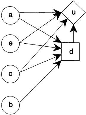
Consider the fully observable influence diagram of Figure 2. Suppose each of the random and decision nodes rep­ resent a binary variable. In this influence diagram, if we were to naively apply a dynamic programming procedure, we would optimize the decision d for each of the 24 = 16 values of the parents. Just by looking at this diagram we can see that we do not need to consider the values of b (this is known as 'barren node removal' [Shachter, 1986]). Thus we really only need to consider the 23 = 8 values of the parents of b. What is presented in this paper is like the bar­ ren node removal, but for specific instances of the parents (e.g., the value of e may be irrelevant for a particular value of b).

Consider the corresponding ICLoT theory. Here we con­ sider the two values of a to be represented as a1 and a2. a1 is thus the proposition that says that a has one value, and a2 is the proposition that says that a has the other value. The other variables are treated analogously.

The value of Po is irrelevant for the example. Suppose, that the rule-base representation is of the form:

When a1 is true, c and b are irrelevant to the utility. When a2 1\ e2 1\ c2 is true then the decision is irrelevant. There is even more pruning that can be carried out when we take dominated strategies into account.

5.1 .2 Finding optimal policies

The fully observable case is where either C1 is empty or there is one decision d e C1 (the 'last' decision) where 1r(d) = C- {d}, and when this decision is removed, the remaining theory is fully observable. This case is consid­ ered first; the general, partially observable, case will be a modification of this case.

Suppose the last decision is { d1 , · · · , dk } E C1.

Consider for each u for which there are rules forutility(u), a covering and exclusive set of explanations of utility( u ) . The explanations form a partition on the set of possible worlds (each possible world will have exactly one explana­ tion true). For each explanation there are two cases:

1. N o di is in the explanation. In this case, when this ex­ planation is true, it doesn't matter which decision is made . For example, in the example above { a2, e2, c2} is an explanation of a utility that does not involve ei­ ther d1 or d2. When a2/\e2/\c2 is true it doesn't matter which decision is made.
2. For all of the other cases, we treat an explanation as a triple ( di , 8 , u) if 8 U { di} is an explanation for utility(u). If this is the case then the algorithm ofFig­ ure 3 will compute the optimal policy. The algorithm repeatedly removes dominated explanations and splits explanations where finer distinctions are needed.

At the end of the algorithm, the resulting explanations corresponds to an optimal policy with (di, 8, u) mean­ ing "do di if 8 is true, and u will be the utility". If more than one of the 8i is true, it doesn't matter which ac­ tion is chosen (either the actions will be the same or the utilities will be the same). The 8i will cover all of the cases not covered in case 1 above.

The worst case of this algorithm occurs when we have to split on all alternatives - this is the same as enumerating all states of the observables.

In our example above, for the case where the decision mat­ ters (i.e., for all cases except when a2 1\ e2 1\ c2) we have the following explanations:

Explanations (2) and (3) are dominated by (1) and can be removed. (5) is dominated by (6) and can be removed. (4) is dominated by (7) and can be removed. We split (7) on { e1, e2}, resulting in explanations ( d1 , { a2, e1 , c1}, 7) and (d1o {a2, e2, c1 }, 7), the latter of which can be pruned as it is dominated by (8).

procedure optimize( S):

input: set S of tuples of the form ( d;, 0, u), such that whenever composite choice 0 is true, decision d; has utility u.

output: set S of tuples of the form ( d;, 0, u), such that whenever 0 is true, decision d; has utility u, and d; is an optimal decision when 0 is true.

1. Remove all dominated explanations from S. If we have two elements (d;, 0;, u;) and { dj, Oj, u i ) inS where u; $ u i and Oj � 0;, then remove (d;, 0;, u;). Ifu; = Uj andOi = 0; then remove either one. [Whenever 0; is true, we know that d i is better than d;, and so we don't need to consider d;.]
2. If there are no dominated elements, and if there are two elements (d;, 0;, v;) e Sand (dh Oi, vi) e S such that 0; U Oi is consistent, d; :F dj and v; < vi do the following: Select o e Oi 0;. Suppose o is in observation alternative 0. Replace (d;, 0;, v;) inS by the split of (d;, 0;, v; ) on 0. Go to step 1.
3. If neither case 1 nor case 2 is applicable, return S .

Figure 3: Finding optimal policies from observations

1be resulting explanations are:

(db{at}, 7) (d2, {a2, el, c2}, 6) (dt, {a2, e l, c1}, 7) (d2, {a2, e2, c1 }, 9)

This can be interpreted as an optimal policy, which says that when a1 is true do d1, when a2 1\ e1 1\ c2 is true do d2, etc. When none of the cases occur (i.e., when a2 1\ e2 1\ c2 is observed) it doesn't matter which action is taken.

5.2 Partially Observable Single Decision

The partially observable single decision case consists of 4 steps:

1. finding explanations of utility(U) for each value U and explanations for the observables, using expl;
2. repeated removing of dominated explanations and case analysis on relevant observations;
3. computed expected utilities for the relevant cases of observations and
4. using the optimize algorithm of Figure 3 to generate an optimal strategy.

Suppose we have the last decision d = { d1 , . . . , d,.} e C1. Dynamic programming would tell us that we have to con­ sider each case of expansion( 1r( d)) (the set of all value as­ signments to the 'parents' of d)there are exponentially many of these (in the size of 1r(d)). We would like to con­ sider each observable in 1r( d) separately, to see when it is relevant to the decision being made . This is done by the use ofre:

Definition 5.1 If 0 E 1r{d) let re ( O ) = {(o, expl(o)) : o E 0}. re ( O ) is a representation for the explanations of the possible observations in 0. We assume that for each 0 e 1r(d), that the function re ( O ) is computed once and stored.

Example 5.2 Consider the example of Section 2.1.

For the last decision, namely { d{O), d(l), d(2) }, and for each 'observable', we determine the re function which tells us what it is that the sensors detect:

re( { ta(hi), ta(low)}) = { (ta(hi), { { ta(hi) }}) , (ta(lo), { { ta(lo)} })} re ( {as(pos), as(neg)}) = {(as(pos), {{ ta(hi), a( hi)}, { ta(lo), a(lo)} }) , (as( neg), { { ta(hi), a(lo) }, { a(med)}, {ta(lo), a(hi)}})} re ( {bs(pos), bs(neg)}) = {(bs(pos ), {{b(pos ), true.pos }, {b(neg), false..pos} }), (bs(neg), { {b(neg), trueJleg}, {b(pos ), falseJleg}})}

These are stored, and are combined with the explanations of different utilities in order to determine the relevant cases.

In general we have to check correlations between the obser­ vations and the cases where one decision is better than the other. The fully observable case showed the idea of to how to isolate the cases where the one decision is better than an­ other.

Definition 5.3 Tuple (d;, 0, K;, u), where 0 is a composite observation and u is a number is a pre-policy if K:, is a set of covering explanations of 0 1\ utility( u) which contains d;. Set Eo of pre-policies is covering if for every world w,. there is a unique (d;, 0, K;, u) E Eo such that dis true in w,. and one explanation in K:, is true in w ...

The algorithm works by maintaining a set of covering pre­ policies. These can be set up using:

Lemma 5.4 The set {(d;, {}, {K, e expl(utility(u)): d; E K-}, u): d; Ed} is a covering set of pre-policies. This can be easily computed by generating expl(utility(u)) for each u for which there are rules.

Example 5.5 Continuing our example, we create the pre­ policies for different utilities, some of which are:

These specify the distinctions that are important to deter­ mine utility.

A basic step is to split pre-policies based on the different possible values of an observable (i.e., we consider each of the cases for the values of the observable):

Lemma 5.6 If (d, 0, lC, u} is a pre-policy, and o E 1r(d) then for all (c, IC'} E ce( o ), (d, (} U { c }, 1C ® lC', u} is a pre­ policy.

We only want to do case analysis with respect to an obser­ vation if it is relevant. The notion of 'autonomous' gives a syntactic criteria for determining if an observation is rele­ vant:

Definition 5. 7 If K:1 and K:2 are sets of composite choices then 1C1 and 1C2 are autonomous if 'VK1 E 1C1 'VK2 E K:2 'Vc1 E K1 'Vc2 E K2 ,liA E C {e l l c2} � A. Thus they are autonomous if they involve different alternatives.

The following le mma can be easily proved:

Lemma 5.8 If the set of explanations of g1 and the set of explanations of Y2 are autonomous then Y1 and Y2 are inde­ pendent.

We can stop expanding on observations when all other ob­ servations are irrelevant.

Definition5.9 Pre-policy {d;,0I,K1,u} is observation full if for every 02 E 1r(d) either 02 n 01 -::f: {} or for all (c, K2} E ce(02) , K2 and K1 are autonomous.

If pre-policy ( d, 0, K1, u} is observation full, then the other observations are irrelevant to decision d in the context of observation (}.

Example 5.10 Continuing example 5.5, partial explana­ tion (9) is observation full: for action d(O) all observations are irrelevant as far as the utility is concerned.

Partial explanation (10) is autonomous of ce( {ta(hi), ta(low)}) andre ( {bs(pos}, bs(neg) }, but is not autonomous of ce( {as(pos), as( neg)}).

Figure 4 given a procedure for expanding a set of pre­ policies to an equivalent set that is observation-full. In the worst case, the set produced will contain one element for each element of d and each element of expansion(1r(d)). In many cases this will be much smaller. This algorithm procedure expand(S):

input: set S of pre-policies.

output: set of observation full pre-policies.

1. Select (d;, 0, K:, u) E Sand 0 E 1r(d) such that 0 n 0 = {} and there is one (c, IC'} E ce( 0) where lC' and 1C are not autonomous. S := S-{(d;, 0, lC, u}} U {(d;,O U {c},K: ® lC', u}: (c, IC'} E ce( 0)}. Go to step 1.
2. If there are no choices in case 1, returnS.

Figure 4: Expanding observations to cover all potentially relevant cases

contains a selection-the algorithm will be correct no mat­ ter which elements (that satisfy the conditions) are selected. Different selections may change the size of the resulting set (e.g., of one observation gives more information than an­ other, this observation should be selected first). Also note that the case analysis we do for the observations is not sym­ metric - one observation may only be relevant for partic­ ular values of other observations.

Example 5.11 Partial explanation (10) needs to be com­ bined with ce( { as(pos), as( neg)}) resulting in:

These can the be combined with ce( { ta(hi), ta(low)} producing:

Which are then observation full. For decision d ( 1) value of bs is irrelevant.

Once we have an observation full set of pre-policies, we can then compute expected values (of the utility given decisions and observations), using the algorithm of Figure 5. Com­ puting expected values is complicated by the fact that for a d; the pre-policies involving different utility values may in­ volve a different split on the observations. This algorithm computes expected utilities for combinations of values of observables, splitting cases when necessary. This proce­ dure treats the expectation calculation as one big sum; in any real implementation we would use some of the more efficient Bayesian network algorithms (such as clique-tree propagation).

Given the expected utilities of the observables, we essen­ tially have the fully observable case from which we can then use optimize of Figure 3 to derive the optimal policy.

procedure expectation( S): input: set of observation full pre-policies. output: set of tuples of the form ( d;, K., v } , such that when­ ever K; is observed, decision d; has (expected) utility v.

Let

Figure 5: Computing Expectations

The general algorithm is now to compute the policy via:

Then 81 corresponds to the optimal policy.

5.3 Multiple Decisions

We assume that there is a 'last' decision d = { dt, ... , d�e} E C1, such that all other decisions that are part of an explanation of utility which contain d are in 1r ( d) (i.e., are 'observable'). If there is no such decision, then we cannot optimize the decisions one at a time [Zhang et al., 1994].

The idea of the algorithm for multiple decisions is the stan­ dard one: we solve the last decision and either replace it with a deterministic function corresponding to the policy (by adding the corresponding rules to :F), or by replacing the rules for utility by new rules that give the expected util­ ity for the optimal policy [Zhang et al., 1994].

5.4 Refinements

There are many refinements that can be given to the above procedure. A few are ru>teworthy:

1. We want to do subsumption as early as possible. Sub­ sumption can be made as early as the expand proce­ dure. Note that, for those cases where all alternatives have been subsumed, neither the expectation proce­ dure nor the optimize procedure need to do any split­ ting.
2. We really want to compute the explanations and the other procedures in a lazy fashion - only expanding enough to see what can be pruned. We want to prune early and prune often!
3. Although we have specified expl here as an abstract procedure, it can be computed top-down (as in [Poole, 1993a]), bottom-up (as in an ATMS), and we are also exploring exploiting structure in a rule-based version of clique-tree propagation.

6 Conclusion

This paper presented one step in a combination of logic and probability.

This paper has proposed a mechanism for reducing the case analysis of dynamic programming. We have exploited the rule structure of the I CLoT in order to determine the cases where some observations are irrelevant

The use of rule structure (called ·tree-structure' there) for Markov decision processes has been explored by Boutilier and colleagues [Boutilier et al., 1995]. Their algorithm is similar to the 'fully observable' case of section 5.1. This paper expands on this to only consider appropriate group­ ings of observations.

Smith et. al [Smith et al., 1993] have explored the use of tree-like definitions for the conditional probability tables in influence diagrams. The difference to this work is that we only have rules plus independent choices - the influence diagram is just one of the representations we can represent. The algorithms are also very different, with Smith et al. us­ ing a variant of Shacbter's algorithm.

This is a part of a project to create a mix of logic and deci­ sion theory, where we can exploit as much of the structure as possible to gain efficiencies. This paper has only scratched the surface of the issues. Currently under development (or under consideration) are rule�based variants (that can ex­ ploit the propositional independence inherent in a rule base) of common probabilistic algorithms for MDPs [Boutilier et al., 1995], influence diagrams (this paper), POMDPs and even a rule-based version of clique-tree propagation.

The representation used here is also of interest in its own right in providing logical variables that can be used for dynamic construction of decision networks (as in [Poole, 1993b]), and can be extended into multiple agents [Poole, 1995bl.

Acknowledgements

This work was supported by Institute for Robotics and In­ telligent Systems, Project IC-7 and Natural Sciences and Engineering Research Council of Canada Operating Grant OGP0044121. Thanks to Craig Boutilier for valuable dis­ cussions and for co mme nts on earlier versions of this pa­ per.

References

• [Apt and Bezem, 1991] K. R. Apt and M. Bezem. Acyclic programs. New Generation Computing, 9(3-4):335-363, 1991.
• [Ballard, 1983] B. W. Ballard. The *-minimax search pro­ cedure for trees containing chance nodes. Artificial In­ telligence, 21(3):327-350, 1983.
• [Boutilier et al., 1995] C. Boutilier, R. Dearden, and M. Goldszmidt. Exploiting structure in policy construc­ tion. In Proc. 14th International Joint Conf. on Artificial Intelligence, to appear, Montreal, Quebec, 1995.
• [Cassandra et al., 1994] A. R. Cassandra, L. Pack Kae­ bling, and M. L. Littman. Acting optimally in partially observable stochastic domains. In Proc. 12th National Conference on Artificial Intelligence, pages 1023-1028, Seattle, 1994.
• [Cooper, 1988] G. F. Cooper. A method for using belief netwoks as influence diagrams. In Proc. Fourth Confer­ ence on Uncertainty in Artificial Intelligence, pages 5563, Minnesota, Minneapolis, 1988.
• [Howard and Matheson, 1981] R. A. Howard and J. E. Matheson. Influence diagrams. In R. A. Howard and J. Matheson, editors, The Principles and Applications of Decision Analysis, pages 720-762. Strategic Decisions Group, CA, 1981.
• [Monahan, 1982] G. E. Monahan. A survey of partially observable Markov decision processes: Theory, models and algorithms. Management Science, 28:1-16, 1982.
• [Pearl, 1988] J. Pearl. Probabilistic Reasoning in Intelli­ gent Systems: Networks of Plausible Inference. Morgan Kaufmann, San Mateo, CA, 1988.
• [Poole, 1993a] D. Poole. Logic programming, abduction and probability: A top-down anytime algorithm for com­ puting prior and posterior probabilities. New Generation Computing, 11(3-4):377-400, 1993.
• [Poole, 1993b] D. Poole. Probabilistic Hom abduction and Bayesian networks. Artificial Intelligence, 64(1):81129, 1993.
• [Poole, 1995a] D. Poole. Abducing through negation as failure: Stable models within the independent choice logic. Technical Report, Department of Computer Science, UBC, ftp://ftp.cs.ubc.ca/ftpllocallpoole/papers/ abnaf.ps.gz, January 1995.
• [Poole, 1995b] D. Poole. Sensing and acting in the independent choice logic. In Working Notes AAAI Spring Symposium 1995- Extending Theories of Ac­ tions: Formal Theory and Practical Applications, ftp:// ftp.cs.ubc.ca/ftpllocallpoole/papers/actions.ps.gz, 1995.
• [Qi and Poole, 1995] R. Qi and D. Poole. New method for influence diagram evaluation. Computational Intel­ ligence, 11(3), 1995.
• [Reiter, 1987] R. Reiter. A theory of diagnosis from first principles. Artificial Intelligence, 32(1):57-95, April 1987.
• [Reiter, 1991] R. Reiter. The frame problem in the situa­ tion calculus: A simple solution (sometimes) and a com­ pleteness result for goal regression. In V. Lifschitz, edi­ tor, Artificial Intelligence and the Mathematical Theory of Computation: Papers in Honor of John McCarthy, pages 359-380. Academic Press, San Diego, 1991.
• [Shachter and Peot, 1992] R. ShachterandM. A. Peot. De­ cision maiking using probabilistic inference methods. In Proc. Eighth Conf. on Uncertainty in Artificial Intelli­ gence, pages 276-283, Stanford, CA, 1992.
• [Shachter, 1986] R. D. Shachter. Evaluating influence diagrams. Operations Research, 34(6):871-882, November-December 1986.
• [Smith et al., 1993] J. E. Smith, S. Holtzman, and J. E. Matheson. Structuring conditional relationships in in­ fluence diagrams. Operations Research, 41 (2):280-297, 1993.
• [Zhang et al., 1994] N. L. Zhang, R. Qi, and D. Poole. A computational theory of decision networks. Inter­ national Journal of Approximate Reasoning, 11(2):83158, 1994.