Faithful Approximations of Belief Functions

David Harmanec

Medical Computing Laboratory Department of Computer Science School of Computing National University of Singapore Lower Kent Ridge Road Singapore 119260

Abstract

A conceptual foundation for approximation of belief functions is proposed and investi­ gated. It is based on the requirements of consistency and closeness. An optimal ap­ proximation is studied. Unfortunately, the computation of the optimal approximation turns out to be intractable. Hence, various heuristic methods are proposed and exper­ imantally evaluated both in terms of their accuracy and in terms of the speed of com­ putation. These methods are compared to the earlier proposed approximations of belief functions.

outcome space). Most algorithms involving belief func­ tions (or their various transformations) have compu­ tational complexity polynomial in the number of focal elements. However, some algorithms may produce a belief function with a larger number of focal elements than the number of focal elements of its input belief function(s). Moreover, the original belief function may itself have more focal elements than the prescribed limit. To solve this problem we need a method that would efficiently produce ideally the best, or at least a good, approximation of a given general belief func­ tion. Addressing the development of such methods is the topic of the current paper.

1 INTRODUCTION

It is now widely accepted fact that many situations involving uncertainty cannot be very well represented within classical probability framework. Ignorance, lack of time, or a small sample size are just a few of the reasons making it hard, if not impossible, to obtain reliable point probabilities. One may then ask why the various theories of imprecise probabilities are so rarely applied to solve practical problems compared to the classical probability theory. I believe, the explanation lies in the fact that, in general, using imprecise proba­ bilities has the computational complexity exponential in the size of the set of possible alternatives consid­ ered while using classical probabilities is only linear in the size of the universal set. Hence, the price for better accuracy or reliability seems too high. A pos­ sible solution of this dilemma is to use a subclass of imprecise probabilities that is expressive enough and at the same time inferences within this subclass are computationally tractable.

One possible candidate for such a class is the class of belief functions with the number of focal elements limited by a small constant (e.g., twice the size of the

This work is by no means the first attempt to develop an approximation method for belief functions. Previ­ ous work can be divided into two streams. One type of proposal was to approximate a given belief function by either a probability or possibility measure [3, 4, 17]. While it might be useful method for utilizing some of the existing techniques from probability and possibil­ ity theories on input in the form of belief function(s), it hardly qualifies as a general approximation method. The reason is that the structure of both probability and possibility measures is very simple and hence too restrictive from the point of view of belief functions. In general, it is possible to allow a more general structure of the approximating belief function while preserving the same computational complexity. Approximating belief functions by probability measures also intro­ duces "information" that is not present in the original belief function 1 . The other direction of the research on approximation of belief functions focused on the devel­ opment of a general approximation method. However, the proposals found in the literature [16, 1, 2] are not based on a well-founded approach to approximation. They are evaluated only on the basis of computer ex­ periments using questionable measure( s) of goodness

1 Although it is possible to preserve the amount of infor­ mation carried by both the belief function and the proba­ bility measure [5].

of approximation. I discuss these proposals in detail in Section 4.1. I should also mention that Monte-Carlo techniques have been applied to reasoning with belief functions (8].

Another approach to reduction of computational com­ plexity found in the literature is to use a factorization of belief functions over a hypertree of sets of variables and a local computation algorithm to reason with the belief functions (7, I3, 10]. This approach is indepen­ dent of using approximations and could be used in combination with it.

2 PRELIMINARIES

Let X = { x 1 , x2, ... , xn} denote a finite and non­ empty universal set, usually referred to as a frame of discernment in the Dempster-Shafer theory [I2), and let P (X) denote the power set of X.

A function Bel : P (X) -+ [ 0, I], which satisfies Bel (0) = 0, Bel (X) = I, and

where the summation goes over all 0 of I � {I, ... , N} for all positive integers N and all {A;} ;:1 � P (X), is called a belief function.

A function PI : P (X) -t [ 0, I] is called a plausibility function if it satisfies PI (0) = 0, Pl (X) = I, and

where the summation goes over all 0 of I � {I, ... , N} for all positive integers Nand all {A;};:1 s; P (X).

A basic probability assignment is a function m : P (X) -t [0, I] such that m (0) = 0 and L:Ae"P(X) m (A) = I. A subset A of X such that m (A) > 0 is called a focal element of m.

It is well known [I2) that there are one-to-one corre­ spondences between belief functions, plausibility func­ tions and basic probability assignments. Due to these correspondences we can freely use any of them in our argumentation. Moreover, any notion associated with any of the functions rn, Bel or Pl naturally translates to the remaining two by these correspondences. For example, we can talk about focal elements of a belief function meaning focal elements of its associated basic probability assignment.

In the algorithms in this paper, a basic probability assignment m is represented as a set of pairs of all focal elements of m and their corresponding value of basic probability assignment, i.e.,

If a particular set B is not in any pair in rn then m (B) = 0.

3 OPTIMAL APPROXIMATION

In this section, I look into the problem of finding an "optimal" or "best" approximation for a given belief function. A belief function has to satisfy two basic re­ quirements to be considered an approximation. First, it has to be a "simple" belief function. 2 In this pa­ per, a belief function is considered simple, if it has at most k focal elements, where k is a small positive integer. k is intentionally left unspecified as a param­ eter to the approximation method(s). Second, it has to be faithful. For an approximation to be faithful, the inferences made with it should be, in some sense, consistent with the inferences made with the original belief function. For an approximation to be considered best, it has to be the approximation that is the closest to the original. The next two subsections make these notions more precise.

3.1 CONSISTENCY OF BELIEF FUNCTIONS

The faithfulness of the approximation is made precise by the notion of consistency.

Definition 1 Let Bel and Bel' denote two belief func­ tions on X. We say that Bel' is (weakly) consis­ tent with Bel if and only if Bel (A) � Bel' (A) for all A<; X.

The definition states that Bel' is consistent with Bel if it does not ascribe a larger belief than Bel to any subset of X, i.e., Bel is more precise the interval [Bel' (A), Pl' (A)] contains the interval [Bel (A), Pl (A)] for each A<; X. It appears very nat­ ural to ask that an approximation is consistent with the original belief function, no matter what interpreta­ tion of belief functions is used. Some authors (e.g.,[4]) use the name (weak) inclusion instead of consistence for the same property. I prefer the name consistence as it is not tied to the random set interpretation of belief functions.

Although the notion of consistence is very natural, it does not offer a guidance how to actually compute an approximation of a given belief function. The notion of strong consistency, though admittedly less intuitive, offers such a guidance.

21 could consider "approximations" by arbitrarily com­ plex belief functions, but as I am interested in reducing computational complexity, I explicitly exclude complex be­ lief functions from the class of approximations.

Definition 2 Let Bel, Bel' denote two belief function on X and let m, m ' denote their corresponding basic probability assignments. Moreover, let A1, A2, . . . , Ap (p 2: 1) denote all focal elements of m and let B1, B2, · · . , Bq (q 2 1) denote all focal elements of m ' . We say that Bel' is strongly consistent with Bel if and only if there is a collection of numbers Wij, i = 1, 2, ... , p, j = 1, 2, . . . . ,q, such that

and B j i. Ai ==> Wii = 0.

A belief function Bel' is strongly consistent with an­ other belief function Bel if the basic probability as­ signment value of every focal element of Bel' is a sum of fractions of basic probability assignment values of some focal elements of Bel that are its subsets. In other words, (some fractions of) basic probability val­ ues of focal elements of the "original" belief function are moved to a superset in the "approximation". As expected, the strong consistence implies consistence; the inverse does not hold in general (3].

Now we can define precisely what is meant by "ap­ proximation" in this paper.

Definition 3 A belief function Bel' is called (strong) k-approximation of a given belief function Bel if Bel' is (strongly) consistent with Bel and Bel' has at most k focal elements.

3.2 MEASURE OF CLOSENESS

To measure the "closeness" of an approximation, I use the function DFeel defined by

for any belief function Bel' on X consistent with Bel. To obtain the best approximation we need to minimize this function over all (strong) k-approximations of Bel. That is, we try to minimize the sum of differences of a given belief function and the "approximating" belief function.

3.3 AN ALGORITHM FOR COMPUTING AN OPTIMAL APPROXIMATION

In the rest of the paper, I investigate only strong k­ approximations of a given belief function. However, if the following conjecture holds, finding optimal k­ approximation is the same thing as finding optimal strong k-approximation.

Conjecture 1 Let Bel denote a belief function on X. Any belief function Bel' that is consistent with Bel and minimizes DFee l among all the belief functions con­ sistent with Bel is also strongly consistent with Bel.

Our goal is to find optimal strong k-approximation of a given belief function Bel. In general, there may be many optimal strong k-approximations. We want to find at least one. The theorem below suggests where to start looking.

Theorem 1 Let Bel denote a belief function on X and let Bel' denote a strong k-approximation of Bel. Then there exists a strong k-approximation Bel" of Bel such that its focal elements are also focal elements of Bel', (under the notation of Definition 2} w � e l '' E {0, m (A;)} and DFeel (Bel') 2: DFeel (Bel").

As a consequence of the above theorem, we only need to explore the partitions of the set of focal elements of the original belief function into k parts to find the opti­ mal strong k-approximation. The following algorithm is a formalization of this idea.

Algorithm 1 (Optimal approximation)

Input: a basic probability assignment M = { ( B i , m ( B ; ) ) I i = 1, 2, ... ,s}, number of focal elements for the approximation k Output: optimal approximation of M if s 5 k then return M else Find the first partition K = { H, P2, ... , P k} of{1, 2, . . . , s} OPT= { ( UiEP, B i , �iEP, m ( B i ) ) I PtE K, l = 1, 2, . . . , k} while there is an unexamined partition of { 1, 2, ... , s} do Find the next partition K = { P1, P2, ... , P k } of {1, 2, . .. , s } W M = { (UieP, BJ, �JEP, m (BJ ) ) I f} E K, l = 1, 2, . . . ,k} if DF (W M) < DF (OPT) then OPT=WM end if end while return OPT end if

Unfortunately, going through all possible partitions is not computationally tractable.

4 HEURISTIC APPROXIMATIONS

As seen in the previous section, it is not computa­ tionally feasible to find an optimal approximation of a given belief function. As usual in such a situation, one needs to turn to a heuristic method that does not guar­ antee optimal results but empirically provides good ap­ proximations. In this section, I propose several such heuristic methods. I also overview and discuss pro­ posals from the literature for heuristic approximation methods. The experimental evaluation of these meth­ ods is the topic of the next section.

4.1 PREVIOUS WORK

This subsection is an overview of the previous propos­ als for approximations of belief functions. As all the proposals are heuristic methods, I discuss them within a section on heuristic algorithms.

Voorbraak [17) proposed Bayesian approximation of belief functions that approximates given belief func­ tion by a probability measure. It is well known [12) that a probability measure is a special type of be­ lief function with only singleton focal elements. For a given basic probability assignment m the basic prob­ ability assignment m' of the Bayesian approximation of misgiven by

Obviously the Bayesian approximation has at most lXI focal elements. Unfortunately, the Bayesian approxi­ mation is generally not consistent with the original belief function, which is one of our fundamental re­ quirements.3 Bayesian approximation commutes with the Dempster rule of combination, which is its distin­ guishing characteristic.

In my opinion, the most well founded approximation method found in the literature is the consonant ap­ proximation of a belief function proposed by Dubois and Prade [4). Their goal is to find a maximal conso­ nant strongly consistent belief function that maximizes imprecision (i.e., the expression I; m (A) · I AI). This is an NP-hard problem so they proposed a heuristic algorithm as a computationally tractable approxima­ tion. Like the Bayesian approximation, the consonant approximation has at most lXI focal elements. As mentioned above, the consonant approximation is a faithful approximation. Its main limitation is its re­ striction to consonant belief functions. See Section 5

3 This is true for any "approximation" by a probability measure, which also excludes using Smet's pignistic proba­ bility as an approximation (14].

for quantitative comparison with other faithful heuris­ tic methods.

Lowrance et al [9) appear to be the first to pro­ pose a general method, called summarization, for ap­ proximating belief functions. Let m denote a given basic probability assignment with s focal elements A1, A2, ... , A, ordered in such a way that m (A;) � m(Ai+1) for all i E {1,2, . . . ,s -1 } . Then the sum­ marization approximation m' is given by

This approximation is also strongly consistent with the original belief function.

The first systematic study of approximations of belief functions was done by Tessem [16). He also proposed a new method called k-l-x approximation. The k-l-x approximation works by preserving the original focal elements with the highest basic probability assignment values and renormalizing the values. Unfortunately, the resulting belief function is not, in general, consis­ tent with the original belief function. Tessem uses the maximum difference over all subsets of X between the pignistic probability [14] corresponding to the original and approximating belief function as the measure of closeness (or error measure in his terminology). The use of this measure is questionable. There are other possible 'representations' of a belief function by a prob­ ability measure (e.g., maximum entropy probability) and one can also use the belief function directly in decision making [6, 11, 15, 18].

Bauer [1, 2] did a second, and, to my knowledge, last systematic study of approximations of belief functions. He also proposed a new approximation method, called Dl. The Dl approximation works by keeping k- 1 focal elements from the original basic probability as­ signment and distributing the mass from the rest of the focal elements to these or to X. The distri bu­ tion is done either to the minimal supersets if any, or to minimal non-disjoint sets with larger cardinality if any (according to the proportion of their intersec­ tion with the distributed focal element), or to X as the last resort. Again, the Dl approximation method does not always produce a belief function that is con­ sistent with the original belief function. Bauer uses the main Tessem's error measure as well as two new ones. These measures suffer from the same drawbacks as the main Tessem 's error measure as they are also based on the pignistic probability. Moreover, the moti­ vation of these measures is dubious. The author seems to suggest that the user would make the decision on the basis of the highest pignistic probability. How-

ever, this is not the standard decision making set up, when the user has a choice of actions and makes a decision based on utility expectations with respect to probabilities (belief functions) conditional on taking a particular action .

4.2 PAIR APPROXIMATION

The first heuristic approximation method is a varia­ tion of the standard one-step-look-ahead (or greedy) heuristic. It reduces the number of focal elements of the current basic probability assignment by one at each step (starting from the original) until the desired number k of focal elements is reached. The reduction is done by merging the two focal elements, merging of which results in the smallest DFBel, where Bel is the belief function corresponding to the current basic probability assignment. The following result is used in the selection.

Proposition 1 Let m denote a basic probability as­ signment on X and A, B denote two different focal elements of m. Let m' denote a basic probability as­ signment obtained from m by merging A and B, i.e.,

Then

where Bel and Bel' denote, respectively, the belief function corresponding to m and m'.

Let C P (A, B) denote the expression on the left hand side of (2). The algorithm is presented below.

Algorithm 2 (Pair approximation) Input: a basic probability assignment M = {(B;, m(B,)) I i = 1,2, ... , s}, number of focal elements for the approximation k Output: Pair approximation of M if s:::; k then return M else WM=M for (A, m(A)) E WM do c� M = min B I (B,m(B))E{WM -{ (A,m(A))}} C P (A, B) end for while \W M\ > k do B · CWM = argmmAI (A,m{A))EWM A C= arg min AI (A,m(A))E{W M -{ (B ,m(B))}} 0 P (A, B)

4.3 SINGLE APPROXIMATION

The Pair approximation is still quite computationally complex. It has the worst case computational com­ plexity 0 (s3). This is due to the fact that the cost of merging is associated with pairs of focal elements. To reduce the complexity one could try to associate a "cost" with the individual focal elements instead of their pairs, and, at each step, merge the two focal ele­ ments with the lowest "cost" . This is what the Single approximation is doing. Here, the amount of increase of DF by merging a focal element with X is taken as the "cost". From (2) we have

The algorithm is presented below.

Algorithm 3 (Single approximation) Input: a basic probability assignment M = {(B,, m (B;)) I i = 1,2, ... , s}, number of focal elements for the approximation k Output: Single approximation of M if s:::; k then return M else WM=M while IW Ml > k do B = argminA I (A,m(A))EWM OS (A) C= argmin A I (A,m(A))E{WM - {(B,m(B))}} OS (A) WM=(WM{(B, m (B)}, (C, m (C)}, (B u O, m (B u C)}})u {(B u C, m (B) +m (C)+ m (B u C))} end while return WM end if

4.4 RATIO APPROXIMATION

The choice of X as the foci of the merging in the Sin­ gle approximation is somewhat arbitrary. The Ratio approximation goes to the other extreme and com­ putes the "cost" based on the assumption of merging with a superset containing just one extra focal element.

Again, from (2) we have

As we are interested only in the comparison of the values of C R' and C R' (A) < C R' (B) if and only if �liP < ���) , it is simpler to use

instead of CR'. The algorithm of the Ratio approxi­ mation is the same as the algorithm of the Single ap­ proximation with C R replacing C S .

Obviously, one could interpolate between the two ex­ tremes presented by the Single and Ratio approxima­ tions and select a superset with any number of focal elements between IAI + 1 and lXI as the basis of the heuristic "cost". One could even try to select it on the basis of the average size of focal elements in the original. Or, alternatively, one could try to drop using supersets at all. However, I have not pursued these ideas further (yet).

4.5 LUMP APPROXIMATION

If even the speed of the Single or Ratio approxima­ tions is not acceptable, one can use similar idea to that of the summarization method given by (1) and merge all lXI + 1k focal elements with the smallest "cost" in one step instead of doing it iteratively. I call the resulting method the Lump approximation. Let m denote a given basic probability assignment with s focal elements A1, A2, . . . , A, ordered in such a way that CS(Ai) � CS(Ai+l) (or CR(A;) � CR(Ai+l) or any other "cost")4 for all i E { 1 , 2, ... , s1 }. Then the Lump approximation m' is given by

4.6 ITERATIVE APPROXIMATION

The last method I considered is a variation on the "greatest descent" theme. The method starts from a random partition of s focal elements into k parts. The partition corresponds to a belief function consistent with the original belief function the same way as in the case of the optimal approximation. It then iteratively

4 In my experiments I used C S as the "cost" in the Lump approximation.

improves (hence the name Iterative approximation) its current approximation by looking at the neighboring partition until no improvement is possible or the spec­ ified time or number of iterations is exceeded. 5 A par­ tition is neighboring if it can be obtained from the given partition by moving one element from one part to a different part. The exact algorithm follows.

Algorithm 4 (Iterative approximation)

Input: a basic probability assignment M = {(B;,m (B;)) I i = 1, 2, ... , s }, number of focal elements for the approximation k, max.running time Time, max. number of iterations Numlt Output: Pair approximation of M if s:::; k then return M else Find a random partition B!C = { P1, P 2 , . . . , Pk} of {1, 2, ... ,s } BM = {(UjEP, Bi, L:iEP, m (Bj)) I P1 E B!C, l = 1, 2, . . . , k} Numlt = 1 while Time and Numlt is not exceeded do KM=BM !C!C = B!C for pE{1,2, . . . , k} , qE{ 1 , 2 , ... ,k},p#q, IPpl > 1 do for AEPp do K. = ({P1, P2, . . . , Pk}- {Pp, Pq}) U {Pp- {A}, Pq u {A}} WM= { (UjEP,Bi,L:jEP,m(Bj)) I P1 E!C, l= 1,2, ... , k} if DF (W M) < DF (BM) then BM=WM B!C = K. end if end for end for if DF(KM)=DF(BM) then returnBM end if Numlt = Numlt + 1 end while returnBM end if

5 EXPERIMENTS

In this section I report on the experiments I conducted to evaluate the accuracy and speed of the computation

51 did not limit the time or the number of iterations in the experiments.

-

of the heuristic approximation methods I am propos­ ing in this paper as well as the Consonant and Sum­ marization approximations (the only earlier proposals that are faithful). The experimental framework was implemented in C++. Most of the experiments were conducted on a Sun Ultra 1 workstation running So­ laris 2.5, but some were also run on a 166Mhz Pentium MMX PC running Windows 95 to eliminate the pos­ sibility of dependency of the results on the computing platform.

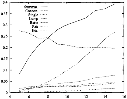
In each run of an experiment, I have randomly gen­ erated 1000 basic probability assignments of a given specification and computed the various heuristic ap­ proximations recording their average scaled D F from the original as well as the average actual time it took to compute them. The minimum and maximum D F of a consistent belief function depends on the original belief function. To get comparable results, I computed the optimal approximation and scaled the DF values of the individual heuristic approximation methods be­ tween the D F of the optimal approximation and the DF of the vacuous belief function (which is trivially consistent) for each original belief function. A huge limitation of this approach is the need to compute the optimal approximation. This can be done only for be­ lief functions with very small number of focal elements. I was able to do it for belief functions with up to 15 fo­ cal elements. In another set of experiments I scaled the D F values only by the D F of the vacuous belief func­ tion. Unlike Tessem ( 16] and Bauer (1, 2], I generated the basic probability assignments uniformly random as I see no compelling reason to do otherwise. To be able to compare the other approximation methods with the Consonant approximation, I used k = lXI in all the ex­ periments, as this requirement is hard-wired into the Consonant approximation. I did the experiments for lXI E {3 , 4, . . . , 8} and for a particular fixed lXI I gen­ erated originals with lXI + 1, lXI + 2, ... , 2 IXI - 1 focal elements. The experiments seem to suggest that the Summarization approximation method is the fastest one to compute but the least (or second least) accu­ rate. The Pair method is the most accurate but the second slowest after the Iterative method. The Itera­ tive method is the only clearly dominated method as for larger number of focal elements it both takes the longest time to compute6 and still is the least (or sec­ ond least) accurate. A sam pie of typical results of the experiments can be found at Figure 1 and Table 1.

60f course, this could be improved by restricting the number of iterations or allocated time. But that would mean further reducing the accuracy of the method.

6 CONCLUSIONS

In this paper, I propose a foundation for approxima­ tions of belief functions. Besides simplicity, consis­ tency with the original and closeness to the original are viewed as basic requirements of an approximation. An algorithm for computing optimal approximation is developed. As the algorithm is not computationally feasible, I suggest several heuristic methods that can be used in practical situations. I also report the results of an experimental evaluation of several heuristic ap­ proximation methods both suggested in this paper and found in the literature. The results show that the Pair approximation is on average the closest to the original from the methods considered and the Summarization approximation of Lowrance et a! (9] takes the shortest time to compute. Somewhat surprisingly and contrary to the previous studies (16, 1, 2] the Consonant approx­ imation of Dubois and Prade (4] does not perform as badly as one might expect. It is my hope that the re­ sults presented here will help to make belief functions a practical alternative to precise probability as a tool for dealing with uncertainty.

Acknowledgments

The work on this paper has been supported by a Strategic Research Grant No. RP960351 from the Na­ tional Science and Technology Board and the Ministry of Education, Singapore.

References

• (1] M. Bauer. Approximations for decision making in the Dempster-Shafer theory of evidence. In E. Horwitz and F. V. Jensen, editors, Proceed­ ings of the Twelfth Annual Conference on Uncer-

Table 1: Sample Average Running Time of Approximations in Seconds (lXI = 4)

s	Summar.	Consonant	Iterative	Lump	Pair	Ratio	Single
5	0.00011	0.00035	0.01076	0.00033	0.00104	0.00023	0. 0001
6	0.00012	0.00032	0.0276	0.00039	0.00196	0.00041	0.00044
7	0.00008	0.00041	0.04837	0.00056	0.00355	0.00072	0.00054
8	0.00016	0.00039	0.07394	0.00078	0.00511	0.00078	0.00096
9	0.00021	0.00054	0.10779	0.00097	0.00723	0.00115	0.00116
10	0.00011	0.00069	0.14258	0.00104	0.00943	0.0016	0.00138
11	0.00009	0.00062	0.18435	0.00126	0.01207	0.00189	0.00182
12	0.00018	0.00075	0.22368	0.00162	0.01509	0.00194	0.00208
13	0.00019	0.00068	0.27124	0.00184	0.01861	0.00228	0.00215
14	0.00024	0. 0008	0.31646	0.00192	0.02239	0.00266	0.00251
15	0.0002	0.00067	0.38495	0.00216	0.0275	0.00289	0.00297

tainty in Artificial Intelligence (UAI-96}, pages 73-80, San Francisco, California, 1996. Morgan Kaufmann.

1. M. Bauer. Approximation algorithms and deci­ sion making in the Dempster-Shafer theory of ev­ idence- An empirical study. International Jour­ nal of Approximate Reasoning, 17{2-3):217-237, 1997.
2. D. Dubois and H. Prade. A set-theoretic view of belief functions: Logical operations and approx­ imations by fuzzy sets. International Journal of General Systems, 12:193-226, 1986.
3. D. Dubois and H. Prade. Consonant approxima­ tions of belief functions. International Journal of Approximate Reasoning, 4{5-6):419-449, 1990.
4. D. Harmanec and G. J. Klir. On information­ preserving transformations. International Journal of General Systems, 26{3):265-290, 1997.
5. J .-Y. Jaffray. Dynamic decision making with be­ lief functions. In Yager et a!. [19], chapter 15, pages 331-352.
6. A. Kong. Multivariate belief functions and graph­ ical models. PhD thesis, Department of Statistics, Harvard University, 1986.
7. V. Y. Kreinovich, A. Bernat, W. Borrett, Y. Mariscal, and E. Villa. Monte-Carlo meth­ ods make Dempster-Shafer formalism feasible. In Yager et a!. [19], chapter 9, pages 175-191.
8. J. D. Lowrance, T. D. Garvey, and T. M. Strat. A framework for evidential-reasoning systems. In T. Kehler, S. Rosenschein, R. Filman, and P. F. Patel-Schneider, editors, Proceedings of the 5th National Conference of the American Association for Artificial Intelligence ( AAAI-86}, volume 2, pages 896-903. AAAI, 1986.
9. K. Mellouli. On the propagation of beliefs in net­ works using the Dempster-Shafer theory of evi­ dence. PhD thesis, School of Business, University of Kansas, 1987.
10. H. T. Nguyen and E. A. Walker. On decision making using belief functions. In Yager et a!. [19], chapter 14, pages 311-330.
11. G. Shafer. A Mathematical Theory of Evidence. Princeton University Press, Princeton, New Jer­ sey, 1976.
12. P. P. Shenoy and G. Shafer. Propagating belief functions with local computations. IEEE Expert, 1:43-52, 1986.
13. P. Smets. Constructing the pignistic probability function in a context of uncertainty. In M. Hen­ rion, R. D. Shachter, and J. F. Lemmer, editors, Uncertainty in Artificial Intelligence, volume 5, pages 29-39. Elsevier Science Publishers, 1990.
14. T. M. Strat. Decision analysis using belief func­ tions. In Yager et a!. [19], chapter 13, pages 275309.
15. B. Tessem. Approximations for efficient compu­ tation in the theory of evidence. Artificial Intel­ ligence, 61(2):315-329, 1993.
16. F. Voorbraak. A computationally efficient ap­ proximation of Dempster-Shafer theory. Interna­ tional Journal of Man-Machine Studies, 30:525 536, 1989.
17. P. Walley. Statistical Reasoning With Imprecise Probabilities. Chapman and Hall, New York, 1991.
18. R. R. Yager, M. Fedrizzi, and J. Kacprzyk, ed­ itors. Advances In The Dempster-Shafer The­ ory Of Evidence. Wiley Professional Computing. John Wiley & Sons, New York, 1994.