Kilian Weinberger Anirban Dasgupta Josh Attenberg John Langford Alex Smola

Yahoo! Research, 2821 Mission College Blvd., Santa Clara, CA 95051 USA

Keywords : kernels, concentration inequalities, document classification, classifier personalization, multitask learning

Abstract

Empirical evidence suggests that hashing is an effective strategy for dimensionality reduction and practical nonparametric estimation. In this paper we provide exponential tail bounds for feature hashing and show that the interaction between random subspaces is negligible with high probability. We demonstrate the feasibility of this approach with experimental results for a new use case - multitask learning with hundreds of thousands of tasks.

1. Introduction

Kernel methods use inner products as the basic tool for comparisons between objects. That is, given objects x 1 , . . . , x n ∈ X for some domain X , they rely on

to compare the features φ ( x i ) of x i and φ ( x j ) of x j respectively.

Eq. (1) is often famously referred to as the kernel-trick . It allows the use of inner products between very high dimensional feature vectors φ ( x i ) and φ ( x j ) implicitly through the definition of a positive semi-definite kernel matrix k without ever having to compute a vector φ ( x i ) directly. This can be particularly powerful in classification settings where the original input representation has a non-linear decision boundary. Often, linear separability can be achieved in a high dimensional feature space φ ( x i ) .

In practice, for example in text classification, researchers

Preliminary work. Under review by the International Conference on Machine Learning (ICML). Do not distribute.

frequently encounter the opposite problem: the original input space is almost linearly separable (often because of the existence of handcrafted non-linear features), yet, the training set may be prohibitively large in size and very high dimensional. In such a case, there is no need to map the input vectors into a higher dimensional feature space. Instead, limited memory makes storing a kernel matrix infeasible.

For this common scenario several authors have recently proposed an alternative, but highly complimentary variation of the kernel-trick, which we refer to as the hashing-trick : one hashes the high dimensional input vectors x into a lower dimensional feature space R m with φ : X → R m (Langford et al., 2007; Shi et al., 2009). The parameter vector of a classifier can therefore live in R m instead of in R n with kernel matrices or R d in the original input space, where m /lessmuch n and m /lessmuch d . Different from random projections, the hashing-trick preserves sparsity and introduces no additional overhead to store projection matrices.

To our knowledge, we are the first to provide exponential tail bounds on the canonical distortion of these hashed inner products. We also show that the hashing-trick can be particularly powerful in multi-task learning scenarios where the original feature spaces are the cross-product of the data, X , and the set of tasks, U . We show that one can use different hash functions for each task φ 1 , . . . , φ | U | to map the data into one joint space with little interference.

While many potential applications exist for the hashingtrick, as a particular case study we focus on collaborative email spam filtering. In this scenario, hundreds of thousands of users collectively label emails as spam or notspam , and each user expects a personalized classifier that reflects their particular preferences. Here, the set of tasks, U , is the number of email users (this can be very large for open systems such as Yahoo Mail TM or Gmail TM ), and the feature space spans the union of vocabularies in multitudes

Feature Hashing for Large Scale Multitask Learning

[email protected] [email protected] [email protected] [email protected] [email protected]

of languages.

This paper makes four main contributions: 1. In section 2 we introduce specialized hash functions with unbiased inner-products that are directly applicable to a large variety of kernel-methods. 2. In section 3 we provide exponential tail bounds that help explain why hashed feature vectors have repeatedly lead to, at times surprisingly, strong empirical results. 3. Also in section 3 we show that the interference between independently hashed subspaces is negligible with high probability, which allows large-scale multi-task learning in a very compressed space. 4. In section 5 we introduce collaborative email-spam filtering as a novel application for hash representations and provide experimental results on large-scale real-world spam data sets.

2. Hash Functions

We introduce a variant on the hash kernel proposed by (Shi et al., 2009). This scheme is modified through the introduction of a signed sum of hashed features whereas the original hash kernels use an unsigned sum. This modification leads to an unbiased estimate, which we demonstrate and further utilize in the following section.

Definition 1 Denote by h a hash function h : N → { 1 , . . . , m } . Moreover, denote by ξ a hash function ξ : N → {± 1 } . Then for vectors x, x ′ ∈ /lscript 2 we define the hashed feature map φ and the corresponding inner product as

Although the hash functions in definition 1 are defined over the natural numbers N , in practice we often consider hash functions over arbitrary strings. These are equivalent, since each finite-length string can be represented by a unique natural number.

/negationslash

Usually, we abbreviate the notation φ ( h,ξ ) ( · ) by just φ ( · ) . Two hash functions φ and φ ′ are different when φ = φ ( h,ξ ) and φ ′ = φ ( h ′ ,ξ ′ ) such that either h ′ = h or ξ = ξ ′ . The purpose of the binary hash ξ is to remove the bias inherent in the hash kernel of (Shi et al., 2009).

/negationslash

In a multi-task setting, we obtain instances in combination with tasks, ( x, u ) ∈ X × U . We can naturally extend our definition 1 to hash pairs, and will write φ u ( x ) = φ ( x, u ) .

3. Analysis

The following section is dedicated to theoretical analysis of hash kernels and their applications. In this sense, the present paper continues where (Shi et al., 2009) falls short: we prove exponential tail bounds. These bounds hold for general hash kernels, which we later apply to show how hashing enables us to do large-scale multitask learning efficiently. We start with a simple lemma about the bias and variance of the hash kernel. The proof of this lemma appears in appendix A.

/negationslash

This suggests that typical values of the hash kernel should be concentrated within O ( 1 √ m ) of the target value. We use Chebyshev's inequality to show that half of all observations are within a range of √ 2 σ . This, together with an indirect application of Talagrand's convex distance inequality via the result of (Liberty et al., 2008), enables us to construct exponential tail bounds.

Lemma 2 The hash kernel is unbiased, that is E φ [ 〈 x, x ′ 〉 φ ] = 〈 x, x ′ 〉 . Moreover, the variance is σ 2 x,x ′ = 1 m ( ∑ i = j x 2 i x ′ j 2 + x i x ′ i x j x ′ j ) , and thus, for ‖ x ‖ 2 = ‖ x ′ ‖ 2 = 1 , σ 2 x,x ′ = O ( 1 m ) .

3.1. Concentration of Measure Bounds

In this subsection we show that under a hashed feature-map the length of each vector is preserved with high probability. Talagrand's inequality (Ledoux, 2001) is a key tool for the proof of the following theorem (detailed in the appendix B).

Theorem 3 Let /epsilon1 < 1 be a fixed constant and x be a given instance such that ‖ x ‖ 2 = 1 . If m ≥ 72 log(1 /δ ) //epsilon1 2 and ‖ x ‖ ∞ ≤ /epsilon1 18 √ log(1 /δ ) log( m/δ ) , we have that

Note that an analogous result would also hold for the original hash kernel of (Shi et al., 2009), the only modification being the associated bias terms. The above result can also be utilized to show a concentration bound on the inner product between two general vectors x and x ′ .

Corollary 4 For two vectors x and x ′ , let us define

Also let ∆ = ‖ x ‖ 2 + ‖ x ′ ‖ 2 + ‖ x -x ′ ‖ 2 . If m Ω( 1 /epsilon1 2 log(1 /δ )) and η = O ( /epsilon1 log( m/δ ) ) , then we have that

The proof for this corollary can be found in appendix C. We can also extend the bound in Theorem 3 for the maximal

canonical distortion over large sets of distances between vectors as follows:

Corollary 5 If m ≥ Ω( 1 /epsilon1 2 log( n/δ )) and η = O ( /epsilon1 log( m/δ ) ) . Denote by X = { x 1 , . . . , x n } a set of vectors which satisfy ‖ x i -x j ‖ ∞ ≤ η ‖ x i -x j ‖ 2 for all pairs i, j . In this case with probability 1 -δ we have for all i, j

This means that the number of observations n (or correspondingly the size of the un-hashed kernel matrix) only enters logarithmically in the analysis.

Proof We apply the bound of Theorem 3 to each distance individually. Note that each vector x i -x j satisfies the conditions of the theorem, and hence for each vector x i -x j , we preserve the distance upto a factor of (1 ± /epsilon1 ) with probability 1 -δ n 2 . Taking the union bound over all pairs gives us the result.

3.2. Multiple Hashing

Note that the tightness of the union bound in Corollary 5 depends crucially on the magnitude of η . In other words, for large values of η , that is, whenever some terms in x are very large, even a single collision can already lead to significant distortions of the embedding. This issue can be amended by trading off sparsity with variance. A vector of unit length may be written as (1 , 0 , 0 , 0 , . . . ) , or as ( 1 √ 2 , 1 √ 2 , 0 , . . . ) , or more generally as a vector with c nonzero terms of magnitude c -1 2 . This is relevant, for instance whenever the magnitudes of x follow a known pattern, e.g. when representing documents as bags of words since we may simply hash frequent words several times. The following corollary gives an intuition as to how the confidence bounds scale in terms of the replications:

1. It is norm preserving: ‖ x ‖ 2 = ‖ x ′ ‖ 2 .
2. It reduces component magnitude by 1 √ c = ‖ x ′ ‖ ∞ ‖ x ‖ ∞ .
3. Variance increases to σ 2 x ′ ,x ′ = 1 c σ 2 x,x + c -1 c 2 ‖ x ‖ 4 2 .

Applying Lemma 6 to Theorem 3, a large magnitude can be decreased at the cost of an increased variance.

3.3. Approximate Orthogonality

For multitask learning, we must learn a different parameter vector for each related task. When mapped into the same hash-feature space we want to ensure that there is little interaction between the different parameter vectors. Let U be a set of different tasks, u ∈ U being a specific one. Let w be a combination of the parameter vectors of tasks in U \{ u } . We show that for any observation x for task u , the interaction of w with x in the hashed feature space is minimal. For each x , let the image of x under the hash feature-map for task u be denoted as φ u ( x ) = φ ( ξ,h ) (( x, u )) .

Theorem 7 Let w ∈ R m be a parameter vector for tasks in U \ { u } . In this case the value of the inner product 〈 w, φ u ( x ) 〉 is bounded by

Proof We use Bernstein's inequality (Bernstein, 1946), which states that for independent random variables X j , with E [ X j ] = 0 , if C > 0 is such that | X j | ≤ C , then

We have to compute the concentration property of 〈 w, φ u ( x ) 〉 = ∑ j x j ξ ( j ) w h ( j ) . Let X j = x j ξ ( j ) w h ( j ) . By the definition of h and ξ , X j are independent. Also, for each j , since w depends only on the hash-functions for U \ { u } , w h ( j ) is independent of ξ ( j ) . Thus, E [ X j ] = E ( ξ,h ) [ x j ξ ( j ) w h ( j ) ] = 0 . For each j , we also have | X j | < ‖ x ‖ ∞ ‖ w ‖ ∞ =: C . Finally, ∑ j E [ X 2 j ] is given by

The claim follows by plugging both terms and C into the Bernstein inequality (5).

Theorem 7 bounds the influence of unrelated tasks with any particular instance. In section 5 we demonstrate the realworld applicability with empirical results on a large-scale multi-task learning problem.

4. Applications

The advantage of feature hashing is that it allows for significant storage compression for parameter vectors: storing w in the raw feature space naively requires O ( d ) numbers, when w ∈ R d . By hashing, we are able to reduce this to O ( m ) numbers while avoiding costly matrix-vector multiplications common in Locally Sensitive Hashing. In addition, the sparsity of the resulting vector is preserved.

The benefits of the hashing-trick leads to applications in almost all areas of machine learning and beyond. In particular, feature hashing is extremely useful whenever large numbers of parameters with redundancies need to be stored within bounded memory capacity.

Personalization One powerful application of feature hashing is found in multitask learning. Theorem 7 allows us to hash multiple classifiers for different tasks into one feature space with little interaction. To illustrate, we explore this setting in the context of spam-classifier personalization.

Suppose we have thousands of users U and want to perform related but not identical classification tasks for each of the them. Users provide labeled data by marking emails as spam or not-spam . Ideally, for each user u ∈ U , we want to learn a predictor w u based on the data of that user solely. However, webmail users are notoriously lazy in labeling emails and even those that do not contribute to the training data expect a working spam filter. Therefore, we also need to learn an additional global predictor w 0 to allow data sharing amongst all users.

Storing all predictors w i requires O ( d × ( | U | +1)) memory. In a task like collaborative spam-filtering, | U | , the number of users can be in the hundreds of thousands and the size of the vocabulary is usually in the order of millions. The naive way of dealing with this is to eliminate all infrequent tokens. However, spammers target this memory-vulnerability by maliciously misspelling words and thereby creating highly infrequent but spam-typical tokens that 'fall under the radar' of conventional classifiers. Instead, if all words are hashed into a finite-sized feature vector, infrequent but class-indicative tokens get a chance to contribute to the classification outcome. Further, large scale spam-filters (e.g. Yahoo Mail TM or GMail TM ) typically have severe memory and time constraints, since they have to handle billions of emails per day. To guarantee a finite-size memory footprint we hash all weight vectors w 0 , . . . , w | U | into a joint, significantly smaller, feature space R m with different hash functions φ 0 , . . . , φ | U | . The resulting hashed-weight vector w h ∈ R m can then be written as:

Note that in practice the weight vector w h can be learned directly in the hashed space. All un-hashed weight vectors never need to be computed. Given a new document/email x of user u ∈ U , the prediction task now consists of calculating 〈 φ 0 ( x ) + φ u ( x ) , w h 〉 . Due to hashing we have two sources of error - distortion /epsilon1 d of the hashed inner products and the interference with other hashed weight vectors

/epsilon1 i . More precisely:

The interference error consists of all collisions between φ 0 ( x ) or φ u ( x ) with hash functions of other users,

/negationslash

/negationslash

/negationslash

To show that /epsilon1 i is small with high probability we can apply Theorem 7 twice, once for each term of (8). We consider each user's classification to be a separate task, and since ∑ v ∈ U,v =0 w v is independent of the hashfunction φ 0 , the conditions of Theorem 7 apply with w = ∑ v =0 w v and we can employ it to bound the second term, ∑ v ∈ U,v =0 〈 φ u ( x ) , φ u ( w v ) 〉 . The second application is identical except that all subscripts '0' are substituted with 'u'. For lack of space we do not derive the exact bounds.

/negationslash

The distortion error occurs because each hash function that is utilized by user u can self-collide:

To show that /epsilon1 d is small with high probability, we apply Corollary 4 once for each possible values of v .

In section 5 we show experimental results for this setting. The empirical results are stronger than the theoretical bounds derived in this subsection-our technique outperforms a single global classifier on hundreds thousands of users. We discuss an intuitive explanation in section 5.

Massively Multiclass Estimation We can also regard massively multi-class classification as a multitask problem, and apply feature hashing in a way similar to the personalization setting. Instead of using a different hash function for each user, we use a different hash function for each class.

(Shi et al., 2009) apply feature hashing to problems with a high number of categories. They show empirically that joint hashing of the feature vector φ ( x, y ) can be efficiently achieved for problems with millions of features and thousands of classes.

Collaborative Filtering Assume that we are given a very large sparse matrix M where the entry M ij indicates what action user i took on instance j . A common example for actions and instances is user-ratings of movies (Bennett & Lanning, ). A successful method for finding common factors amongst users and instances for predicting unobserved actions is to factorize M into M = U /latticetop W . If we have millions of users performing millions of actions, storing U

/negationslash

and W in memory quickly becomes infeasible. Instead, we may choose to compress the matrices U and W using hashing. For U, W ∈ R n × d denote by u, w ∈ R m vectors with

where ( h, ξ ) and ( h ′ , ξ ′ ) are independently chosen hash functions. This allows us to approximate matrix elements M ij = [ U /latticetop W ] ij via

This gives a compressed vector representation of M that can be efficiently stored.

5. Results

We evaluated our algorithm in the setting of personalization. As data set, we used a proprietary email spamclassification task of n = 3 . 2 million emails, properly anonymized, collected from | U | = 433167 users. Each email is labeled as spam or not-spam by one user in U . After tokenization, the data set consists of 40 million unique words.

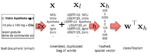
For all experiments in this paper, we used the V owpal Wabbit implementation 1 of stochastic gradient descent on a square-loss. In the mail-spam literature the misclassification of not-spam is considered to be much more harmful than misclassification of spam . We therefore follow the convention to set the classification threshold during test time such that exactly 1% of the not -spam test data is classified as spam Our implementation of the personalized hash functions is illustrated in Figure 1. To obtain a personalized hash function φ u for user u , we concatenate a unique user-id to each word in the email and then hash the newly generated tokens with the same global hash function.

1 http://hunch.net/ ∼ vw/

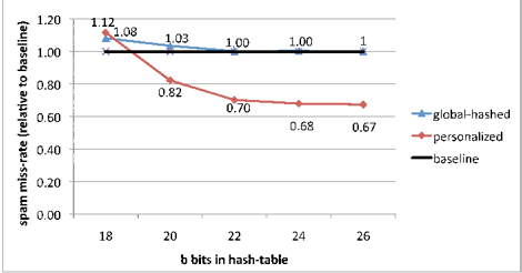
The data set was collected over a span of 14 days. We used the first 10 days for training and the remaining 4 days for testing. As baseline , we chose the purely global classifier trained over all users and hashed into 2 26 dimensional space. As 2 26 far exceeds the total number of unique words we can regard the baseline to be representative for the classification without hashing. All results are reported as the amount of spam that passed the filter undetected, relative to this baseline (eg. a value of 0 . 80 indicates a 20% reduction in spam for the user) 2 .

Figure 2 displays the average amount of spam in users' inboxes as a function of the number of hash keys m , relative to the baseline above. In addition to the baseline, we evaluate two different settings.

The global-hashed curve represents the relative spam catch-rate of the global classifier after hashing 〈 φ 0 ( w 0 ) , φ 0 ( x ) 〉 . At m = 2 26 this is identical to the baseline. Early convergence at m = 2 22 suggests that at this point hash collisions have no impact on the classification error and the baseline is indeed equivalent to that obtainable without hashing.

In the personalized setting each user u ∈ U gets her own classifier φ u ( w u ) as well as the global classifier φ 0 ( w 0 ) . Without hashing the feature space explodes, as the cross product of u = 400 K users and n = 40 M tokens results in 16 trillion possible unique personalized features. Figure 2 shows that despite aggressive hashing, personalization results in a 30% spam reduction once the hash table is indexed by 22 bits.

2 As part of our data sharing agreement, we agreed not to include absolute classification error-rates.

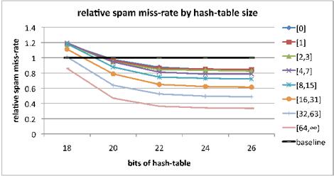
User clustering One hypothesis for the strong results in Figure 2 might originate from the non-uniform distribution of user votes - it is possible that using personalization and feature hashing we benefit a small number of users who have labeled many emails, degrading the performance of most users (who have labeled few or no emails) in the process. In fact, in real life, a large fraction of email users do not contribute at all to the training corpus and only interact with the classifier during test time. The personalized version of the test email Φ u ( x u ) is then hashed into buckets of other tokens and only adds interference noise /epsilon1 i to the classification.

In order to show that we improve the performance of most users, it is therefore important that we not only report averaged results over all emails, but explicitly examine the effects of the personalized classifier for users depending on their contribution to the training set. To this end, we place users into exponentially growing buckets based on their number of training emails and compute the relative reduction of uncaught spam for each bucket individually. Figure 3 shows the results on a per-bucket basis. We do not compare against a purely local approach, with no global component, since for a large fraction of users-those without training data-this approach cannot outperform random guessing.

It might appear rather surprising that users in the bucket with none or very little training emails (the line of bucket [0] is identical to bucket [1] ) also benefit from personalization. After all, their personalized classifier was never trained and can only add noise at test-time. The classifier improvement of this bucket can be explained by the subjective definition of spam and not-spam . In the personalized setting the individual component of user labeling is absorbed by the local classifiers and the global classifier represents the common definition of spam and not-spam. In other words, the global part of the personalized classifier obtains better generalization properties, benefiting all users.

6. Related Work

A number of researchers have tackled related, albeit different problems.

(Rahimi & Recht, 2008) use Bochner's theorem and sampling to obtain approximate inner products for Radial Basis Function kernels. (Rahimi & Recht, 2009) extend this to sparse approximation of weighted combinations of basis functions. This is computationally efficient for many function spaces. Note that the representation is dense .

(Li et al., 2007) take a complementary approach: for sparse feature vectors, φ ( x ) , they devise a scheme of reducing the number of nonzero terms even further. While this is in principle desirable, it does not resolve the problem of φ ( x ) being high dimensional. More succinctly, it is necessary to express the function in the dual representation rather than expressing f as a linear function, where w is unlikely to be compactly represented: f ( x ) = 〈 φ ( x ) , w 〉 .

(Achlioptas, 2003) provides computationally efficient randomization schemes for dimensionality reduction. Instead of performing a dense d · m dimensional matrix vector multiplication to reduce the dimensionality for a vector of dimensionality d to one of dimensionality m , as is required by the algorithm of (Gionis et al., 1999), he only requires 1 3 of that computation by designing a matrix consisting only of entries {-1 , 0 , 1 } . Pioneered by (Ailon & Chazelle, 2006) , there has been a line of work (Ailon & Liberty, 2008; Matousek, 2008) on improving the complexity of random projection by using various code-matrices in order to preprocess the input vectors. Some of our theoretical bounds are derivable from that of (Liberty et al., 2008) .

A related construction is the CountMin sketch of (Cormode & Muthukrishnan, 2004) which stores counts in a number of replicates of a hash table. This leads to good concentration inequalities for range and point queries.

(Shi et al., 2009) propose a hash kernel to deal with the issue of computational efficiency by a very simple algorithm: high-dimensional vectors are compressed by adding up all coordinates which have the same hash value - one only needs to perform as many calculations as there are nonzero terms in the vector. This is a significant computational saving over locality sensitive hashing (Achlioptas, 2003; Gionis et al., 1999).

Several additional works provide motivation for the investigation of hashing representations. For example, (Ganchev &Dredze, 2008) provide empirical evidence that the hash-

ing trick can be used to effectively reduce the memory footprint on many sparse learning problems by an order of magnitude via removal of the dictionary. Our experimental results validate this, and show that much more radical compression levels are achievable. In addition, (Langford et al., 2007) released the Vowpal Wabbit fast online learning software which uses a hash representation similar to that discussed here.

7. Conclusion

In this paper we analyze the hashing-trick for dimensionality reduction theoretically and empirically. As part of our theoretical analysis we introduce unbiased hash functions and provide exponential tail bounds for hash kernels. These give further inside into hash-spaces and explain previously made empirical observations. We also derive that random subspaces of the hashed space are likely to not interact, which makes multitask learning with many tasks possible.

Our empirical results validate this on a real-world application within the context of spam filtering. Here we demonstrate that even with a very large number of tasks and features, all mapped into a joint lower dimensional hashspace, one can obtain impressive classification results with finite memory guarantee.

References

• Achlioptas, D. (2003). Database-friendly random projections: Johnson-lindenstrauss with binary coins. Journal of Computer and System Sciences , 66 , 671-687.
• Ailon, N., & Chazelle, B. (2006). Approximate nearest neighbors and the fast Johnson-Lindenstrauss transform. Proc. 38th Annual ACM Symposium on Theory of Computing (pp. 557-563).
• Ailon, N., & Liberty, E. (2008). Fast dimension reduction using Rademacher series on dual BCH codes. Proc. 19th Annual ACM-SIAM Symposium on Discrete algorithms (pp. 1-9).
• Alon, N. (2003). Problems and results in extremal combinatorics, Part I. Discrete Math , 273 , 31-53.
• Bennett, J., & Lanning, S. The Netflix Prize. Proceedings of KDD Cup and Workshop 2007 .
• Bernstein, S. (1946). The theory of probabilities . Moscow: Gastehizdat Publishing House.
• Cormode, G., & Muthukrishnan, M. (2004). An improved data stream summary: The count-min sketch and its applications. LATIN: Latin American Symposium on Theoretical Informatics .
• Dasgupta, A., Sarlos, T., & Kumar, R. (2010). A Sparse Johnson Lindenstrauss Transform. Submitted .
• Ganchev, K., & Dredze, M. (2008). Small statistical models by random feature mixing. Workshop on Mobile Language Processing, Annual Meeting of the Association for Computational Linguistics .
• Gionis, A., Indyk, P., & Motwani, R. (1999). Similarity search in high dimensions via hashing. Proceedings of the 25th VLDB Conference (pp. 518-529). Edinburgh, Scotland: Morgan Kaufmann.
• Langford, J., Li, L., & Strehl, A. (2007). Vowpal wabbit online learning project (Technical Report). http://hunch.net/?p=309 .
• Ledoux, M. (2001). The concentration of measure phenomenon . Providence, RI: AMS.
• Li, P., Church, K., & Hastie, T. (2007). Conditional random sampling: A sketch-based sampling technique for sparse data. In B. Sch¨ olkopf, J. Platt and T. Hoffman (Eds.), Advances in neural information processing systems 19 , 873-880. Cambridge, MA: MIT Press.
• Liberty, E., Ailon, N., & Singer, A. (2008). Dense fast random projections and lean Walsh transforms. Proc. 12th International Workshop on Randomization and Approximation Techniques in Computer Science (pp. 512-522).
• Matousek, J. (2008). On variants of the JohnsonLindenstrauss lemma. Random Structures and Algorithms , 33 , 142-156.
• Rahimi, A., & Recht, B. (2008). Random features for largescale kernel machines. In J. Platt, D. Koller, Y. Singer and S. Roweis (Eds.), Advances in neural information processing systems 20 . Cambridge, MA: MIT Press.
• Rahimi, A., & Recht, B. (2009). Randomized kitchen sinks. In L. Bottou, Y. Bengio, D. Schuurmans and D. Koller (Eds.), Advances in neural information processing systems 21 . Cambridge, MA: MIT Press.
• Shi, Q., Petterson, J., Dror, G., Langford, J., Smola, A., Strehl, A., & Vishwanathan, V. (2009). Hash kernels. AISTATS 12 .
• Weinberger, K., Dasgupta, A., Attenberg, J., Langford, J., &Smola, A. (2009). Feature hashing for large scale multitask learning. 26th International Conference on Machine Learning (p. 140).

A. Mean and Variance

Proof [Lemma 2] To compute the expectation we expand

Since E φ [ 〈 x, x ′ 〉 φ ] = E h [ E ξ [ 〈 x, x ′ 〉 φ ]] , taking expectations over ξ we see that only the terms i = j have nonzero value, which shows the first claim. For the variance we compute E φ [ 〈 x, x ′ 〉 2 φ ] . Expanding this, we get:

This expression can be simplified by noting that:

Passing the expectation over ξ through the sum, this allows us to break down the expansion of the variance into two terms.

/negationslash

/negationslash

/negationslash by noting that E h [ δ h ( i ) ,h ( j ) ] = 1 m for i = j . Using the fact that σ 2 = E φ [ 〈 x, x ′ 〉 2 φ ] -E φ [ 〈 x, x ′ 〉 φ ] 2 proves the claim.

/negationslash

B. Concentration of Measure

We use the concentration result derived by Liberty, Ailon and Singer in (Liberty et al., 2008). Liberty et al. create a Johnson-Lindenstrauss random projection matrix by combining a carefully constructed deterministic matrix A with random diagonal matrices. For completeness we restate the relevant lemma. Let i range over the hashbuckets. Let m = c log(1 /δ ) //epsilon1 2 for a large enough constant c . For a given vector x , define the diagonal matrix D x as ( D x ) jj = x j . For any matrix A ∈ /Rfractur m × d , define ‖ x ‖ A ≡ max y : ‖ y ‖ 2 =1 ‖ AD x y ‖ 2 .

Lemma 2 (Liberty et al., 2008). For any columnnormalized matrix A , vector x with ‖ x ‖ 2 = 1 and an i.i.d. random ± 1 diagonal matrix D s , the following holds: ∀ x, if ‖ x ‖ A ≤ /epsilon1 6 √ log(1 /δ ) then, Pr[ |‖ AD s x ‖ 2 -1 | > /epsilon1 ] ≤ δ.

We also need the following form of a weighted balls and bins inequality - the statement of the Lemma, as well as

/negationslash the proof follows that of Lemma 6 (Dasgupta et al., 2010). We still outline the proof because of some parameter values being different.

Lemma 8 Let m be the size of the hash function range and let η = 1 2 √ m log( m/δ ) . If x is such that ‖ x ‖ 2 = 1 and ‖ x ‖ ∞ ≤ η , then define σ 2 ∗ = max i ∑ d j =1 x 2 j δ ih ( j ) where i ranges over all hash-buckets. We have that with probability 1 -δ ,

Proof We outline the proof-steps. Since the buckets have identical distribution, we look only at the 1 st bucket, i.e. at i = 1 and bound ∑ j : h ( j )=1 x 2 j . Define X j = x 2 j ( δ 1 h ( j ) -1 m ) . Then E h [ X j ] = 0 and E h [ X 2 j ] = x 4 j ( 1 m -1 m 2 ) ≤ x 4 j m ≤ x 2 j η 2 m using ‖ x ‖ ∞ ≤ η . Thus, ∑ j E h [ X 2 j ] ≤ η 2 m . Also note that ∑ j X j = ∑ j : h ( j )=1 x 2 j -1 m . Plugging this into the Bernstein's inequality, equation 5, we have that

By taking union bound over all the m buckets, we get the above result.

Proof [Theorem 3] Given the function φ = ( h, r ) , define the matrix A as A ij = δ ih ( j ) and D s as ( D s ) jj = r j . Let x be as specified, i.e. ‖ x ‖ 2 = 1 and ‖ x ‖ ∞ ≤ η . Note that ‖ x ‖ φ = ‖ AD s x ‖ 2 . Let y ∈ /Rfractur d be such that ‖ y ‖ 2 = 1 . Thus

by applying the Cauchy-Schwartz inequality, and using the definition of σ ∗ . Thus, ‖ x ‖ A = max y : ‖ y ‖ 2 =1 ‖ AD x y ‖ 2 ≤ σ ∗ ≤ √ 2 m -1 / 2 . If m ≥ 72 /epsilon1 2 log(1 /δ ) , we have that ‖ x ‖ A ≤ /epsilon1 6 √ log(1 /δ ) , which satisfies the conditions of Lemma 2 from (Liberty et al., 2008). Thus applying the above result from Lemma 2 (Liberty et al., 2008) to x , and

using Lemma 8, we have that Pr[ |‖ AD s x ‖ 2 -1 | ≥ /epsilon1 ] ≤ δ and hence

by taking union over the two error probabilities of Lemma 2 and Lemma 8, we have the result.

C. Inner Product

Proof [Corollary 4] We have that 2 〈 x, x ′ 〉 φ = ‖ x ‖ 2 φ + ‖ x ′ ‖ 2 φ -‖ x -x ′ ‖ 2 φ . Taking expectations, we have the standard inner product inequality. Thus,

Using union bound, with probability 1 -3 δ , each of the terms above is bounded using Theorem 3. Thus, putting the bounds together, we have that, with probability 1 -3 δ ,

D. Refutation of the Previous Incorrect Proof

There were a few bugs in the previous version of the paper (Weinberger et al., 2009). We now detail each of them and illustrate why it was an error. The current result shows that the using hashing we can create a projection matrix that can preserve distances to a factor of (1 ± /epsilon1 ) for vectors with a bounded ‖ x ‖ ∞ / ‖ x ‖ 2 ratio. The constraint on input vectors can be circumvented by multiple hashing, as outlined in Section 3.2, but that would require hashing O ( 1 /epsilon1 2 ) times. Recent work (Dasgupta et al., 2010) suggests that better theoretical bounds can be shown for this construction. We thank Tamas Sarlos and Ravi Kumar for the following writeup on the errors and for suggestion the new proof in Appendix B.

1. The statement of the main theorem in Weinberger et al. (Weinberger et al., 2009, Theorem 3) is false as it contradicts the lower bound of Alon (Alon, 2003). The flaw lies in the probability of error in (Weinberger et al., 2009, Theorem 3), which was claimed to be exp( -√ /epsilon1 4 η ) . This error can be made arbitrarily small without increasing the embedding dimensionality m but by decreasing η = || x || ∞ || x || 2 , which in turn can be achieved by preprocessing the input vectors x . However, this contradicts Alon's lower bound on the em-

bedding dimensionality. The details of this contradiction are best presented through (Weinberger et al., 2009, Corollary 5) as follows.

/negationslash

Set m = 128 and δ = 1 / 2 and consider the vertices of the n -simplex in /Rfractur n +1 , i.e., x 1 = (1 , 0 , ..., 0) , x 2 = (0 , 1 , 0 , ..., 0) , . . . . Let P ∈ /Rfractur ( n +1) c × ( n +1) be the naive, replication based preconditioner, with replication parameter c = 512log 2 n as defined in Section 2 of our submission or (Weinberger et al., 2009, Section 3.2). Therefore for all pairs i = j we have that || Px i -Px j || ∞ = 1 / √ c and that || Px i -Px j || 2 = √ 2 . Hence we can apply (Weinberger et al., 2009, Corollary 5) to the set of vectors Px i with η = 1 / √ 2 c = 1 / (32 log n ) ; then the claimed approximation error is √ 2 m +64 η 2 log 2 n 2 δ = 1 8 + 1 16 ≤ 1 4 . If Corollary 5 were true, then it would follow that with probability at least 1 / 2 , the linear transformation A = φ · P : /Rfractur n +1 →/Rfractur m distorts the pairwise distances of the above n + 1 vectors by at most a 1 ± 1 / 4 multiplicative factor. On the other hand, the lower bound of Alon shows that any such transformation A must map to Ω(log n ) dimensions; see the remarks following Theorem 9.3 in (Alon, 2003) and set /epsilon1 = 1 / 4 there. This clearly contradicts m = 128 above.

1. The proof of the Theorem 3 contained a fatal, unfixable error. Recall that δ ij denotes the usual Kronecker symbol, and h and h ′ are hash functions. Weinberger et al. make the following observation after equation (13) of their proof on page 8 in Appendix B.

/negationslash

The quoted observation is false. Let d denote the dimension of the input. Then, ∑ i ∑ j δ h ( j ) i + δ h ′ ( j ) i = ∑ j ( ∑ i δ h ( j ) i + δ h ′ ( j ) i ) = ∑ j 2 = 2 d , independent of the choice of the hash function. Note that t played a crucial role in the proof of (Weinberger et al., 2009) relating the Euclidean approximation error of the dimensionality reduction to Talagrand's convex distance defined over the set of hash functions. Albeit the error is elementary, we do not see how to rectify its consequences in (Weinberger et al., 2009) even if the claim were of the right form.

1. The proof of Theorem 3 in (Weinberger et al., 2009) also contains a minor and fixable error. To see this, consider the sentence towards the end of the proof Theorem 3 in (Weinberger et al., 2009) where 0 < /epsilon1 < 1 and β = β ( x ) ≥ 1 .

Here the authors wrongly assume that √ β 2 + /epsilon1 -β ≥ √ /epsilon1 holds, whereas the truth is √ β 2 + /epsilon1 -β ≤ √ /epsilon1 always.

Observe that this glitch is easy to fix locally, however this change is minor and the modified claim would still be false. Since for all 0 ≤ y ≤ 1 we have that √ 1 + y ≥ 1 + y/ 3 , from β ≥ 1 it follows that √ β 2 + /epsilon1 -β ≥ /epsilon1/ 3 . Plugging the latter estimate into the 'proof' of Theorem 3 would result in a modified claim where the original probability of error, exp( -√ /epsilon1 4 η ) , is replaced with exp( -/epsilon1 12 η ) . Updating the numeric constants in the first section of this note would show that the new claim still contradicts Alon's lower bound. To justify observe that counter example is based on a constant /epsilon1 and the modified claim would still lack the necessary Ω(log n ) dependency in its target dimensionality.