Forecasting Sleep Apnea with Dynamic Network Models

Paul Dagum

Section on Medical Informatics

Stanford University School of Medicine and Rockwell Palo Alto Laboratory 444 High Street Palo Alto, California 94301

Abstract

Dynamic network models {DNMs} are belief networks for temporal reasoning. The DNM methodology combines techniques from time­ series analysis and probabilistic reasoning to provide (1) a knowledge representation that integrates noncontemporaneous and contem­ poraneous dependencies and (2) methods for iteratively refining these dependencies in re­ sponse to the effects of exogenous influences. We use belief-network inference algorithms to perform forecasting, control, and discrete­ event simulation on DNMs. The belief­ network formulation allows us to move be­ yond the traditional assumptions of linearity in the relationships among time-dependent variables and of normality in their proba­ bility distributions. We demonstrate the DNM methodology on an important forecast­ ing problem in medicine. We conclude with a discussion of how the methodology addresses several limitations found in traditional time­ series analyses.

1 INTRODUCTION

Most probabilistic reasoning research has focused on the construction and use of fundamentally static mod­ els, in which custom-tailored temporal relationships are fixed for all times. The predictions of a static model are time invariant in that the model makes the same inferences regardless of when observations are made. The model is memoryless in that it uses only the set of current observations to predict the state of the system.

Although special-case temporal problems can be solved by such static models, in general, a true Bayesian consideration of a complex process unfold­ ing in time must provide a means for representing and updating time-dependent probabilistic relationships. Compared to static models, a truly temporal model is enriched through a consideration of trend informa-

Adam Galper

Section on Medical Informatics Stanford University School of Medicine Stanford, California 94305-5479

tion, and has inferential machinery to update a model in response to changing information about the history of a process. We refer to the adaptation of a model to an ongoing process as dynamic modeling. Failure to adapt. to relevant and emergent trends can severely bias a model.

We have pursued the development of dynamic models for temporal probabilistic reasoning. Such models can be applied to forecasting, control, and discrete-event simulation problems. In this paper, we focus on the task of forecasting, borrowing heavily from statistical forecasting techniques.

Statisticians have developed numerous methods for reasoning about temporal relationships among vari­ ables; the field is generally known as time-series analy­ sis. A time series is a sample realization of a stochas­ tic process, consisting of a set of observations made sequentially over time. Investigators have sought to develop time-series methods for generating or inducing stochastic models, which describe temporal dependen­ cies among successive observations in a time series.

Time-series analyses have been quite successful; a ma­ ture set of Bayesian time-series analysis methods has been developed and applied to a wide range of prob­ lems [15, 31]. However, cla.<>sical time-series method­ ologies are restricted in their ability to represent the general probabilistic dependencies and the nonlineari­ ties of real-world processes. Investigators are forced to wrestle complex problems into relatively simple paranietrized models that can be solved with the tra­ ditional methods. Until recently, there has been rela­ tively little interaction between the statisticians inter­ ested in time-series analysis and the computer scien­ tists studying the representation of uncertain knowl­ edge with Bayesian belief networks.

In this paper, we describe a robust and expressive forecasting procedure based on the integration of fun­ damental methods of Bayesian time-series analysis with belief-network representation and inference tech­ niques. This synthesis, embodied in the dynamic net­ work model ( DNM ) , has two immediate benefits. First, by casting Bayesian time-series analyses as temporal belief-network problems, we can introduce arbitrary

dependency models that capture richer, and more real­ istic, models of dynamic dependencies-as well as the more traditional static (or contemporaneous ) belief­ network dependencies. A robust knowledge represen­ tation can simplify construction of dynamic models by making explicit many of the assumptions in the underlying modeling technique. Second, we can ap­ ply belief-network inference algorithms to the models to generate normative forecasts. The inference algo­ rithms exploit the temporal representation, rendering inference tractable for large belief networks[8]. The richer models and associated computational methods allow us to move beyond such rigid classical assump­ tions as linearity in the relationships among variables and normality of their probability distributions.

We describe an implementation called DYNEMO and val­ idate the DNM forecasting methodology through the analysis of a multivariate time series of 34,000 record­ ings of sleep apnea data 1. Sleep apnea is a serious med­ ical condition, characterized by intermittent periods of arrested breathing during asleep. The National Com­ mission on Sleep Disorders Research, established by Congress in 1988, reported recently that each year the lives of millions of Americans are disturbed, disrupted, or destroyed by the consequences of sleep disorders. The most serious sleep disorder in terms of morbidity and mortality is obstructive sleep apnea [24]. Fore­ casts of apneic episodes could reduce potentially the morbidity and mortality associated with sleep apnea.

2 RELATED WORK

Although most temporal-reasoning research is based on logic (27], several frameworks have been proposed to support temporal reasoning using probability the­ ory. Dean and Wellman (14] provide a good summary of probabilistic models for temporal reasoning and the modeling of dynamic domains. We summarize here some recent results that are relevant to the work pre­ sented.

Berzuini [4] embeds semi-Markov models in a belief­ network representation and uses approximate proba­ bilistic inference to compute the degree of belief in past states and in future states. The inability of these models to adapt to new observations, and their Markov nature, renders them unable to make forecasts that ex­ tend beyond Markov simulation. Dean and Kanazawa [12, 13] develop a probabilistic model for projection based on a functional (e.g., exponential) decay model of the persistence with time of propositions. Kanazawa [20] achieves a synthesis of Bayesian belief networks and elements of the temporal logics of Shoham (26], Bacchus [3], and Halpern (16]. Abramson [2] con-

1 The data were collected from a patient in the sleep laboratory of the Beth Israel Hospital in Boston, Mas­ sachusetts, and made available by the Santa Fe Institute as part of a time-series competition held in the Fall of 1991 [30].

structs a belief-network model for forecasting crude-oil prices where the prior and conditional probabilities are obtained using external regression models. Kjaerulff [23] considers temporal belief networks that consist of a finite number of time slices connected by Markovian dependencies; he describes a more efficient method of junction-tree formation for these networks, but does not address how the model structure and conditional probabilities evolve over time. Approaches that do ad­ dress dynamic modeling with Markovian probabilistic networks include those of Kenley [22] and Tatman and Shachter [28, 29].

3 THE DYNAMIC NETWORK MODEL

Previously we have developed a belief-network-based time-series model called the dynamic network model {DNM) [9]. In this section, we briefly summarize the structure of DNMs, and describe how we employ co n ­ vex combination to specify conditional probabilities.

3.1 STRUCTURE

DNMs consist of nodes which represent domain vari­ ables at different time points-for example, heart rate at timet , HR1 and heart rate at tim e t -1, H R t -1 in Figure 1. Nodes are connected by contemporaneous dependencies if they represent variables at the same time point. Otherwise, nodes are connected by non­ contemporaneous dependencies.

The DNM conditional probabilities are obtained through the convex combination of the contempora­ neous and noncontemporaneous relations. For node X;1, let 7r(X;t) and (}(X;t) denote the sets of contem­ poraneous and noncontemporaneous parents of xit in the DNM, respectively. The convex combination for contemporaneous and noncontemporaneous relations IS

The weight a;1 in Equation 1 lies between 0 and 1, and expresses the relative confidence ascribed to the prior estimate of X;1 and the likelihood provided by the observations. When the weight is close to 1, the prior distribution is more informative than the like­ lihood provided by the observation; when the weight is close to 0, the prior distribution is less informative than the likelihood provided by the observation. Note that the weighting coefficients are time dependent, and the model adapts dynamically to changing exogenous influences by changing the weights.

The method of convex combination may appear ini­ tially to be a naive procedure for integrating histori­ cal information with current estimates of domain vari­ ables. The method, however, embodied in the form of

the Kalman filter in state-space models, and in the conditional sum of squares in ARIMA models [17], is an integral aspect of models that purport to fore­ cast future values of time series. In the absence of prior information, a convex combination is the sim­ plest method of endowing the 'model with the capacity to adapt to changing exogenous influences.

3.2 VALIDITY

In [9) we discuss log-linear decompositions, in addition to convex-combination, as a valuable decomposition of conditional probabilities. In general, we refer to these methods as additive decompositions. In a static model, an additive decomposition of conditional probabilities is an approximation of the true conditional probabil­ ity. In a dynamic model, an additive parametrization is necessary for adaptability to unmodeled exogenous influences.

Additive decompositions overcome two difficult prob­ lems researchers encounter in large belief network ap­ plications [8): intractable inference and intractable in­ duction. The performance of exact inference deterio­ rates rapidly with increasing order because the non­ contemporaneous dependencies yield very large clique sizes. However, Dagum and Galper [8) show that an exact inference algorithm can exploit the additive de­ composition of the conditional probabilities to reduce the complexity of inference in a DNM. The complex­ ity of inference is determined by the size of the largest clique contained in a single time slice, rather than the largest clique of the entire DNM. Similarly, automated induction of a large DNM with Cooper and Herskovits' algorithm (6) is possible if we adapt the algorithm to exploit the additive decomposition. We discuss this point further in Section 5.

3.3 MODEL UPDATE

In time-series analyses, dynamic models adapt to changes in system behavior through the reestimation of model parameters when new observations are made. The process of updating a DNM is the iterative process by which we use new observations to update the esti­ mates of the weighting coefficients in Equation 1. In (10), we consider three methods of update: maximum likelihood, Bayesian update, and maximum expected utility. Maximum expected utility update produced the best forecast results in the analysis of the sleep­ apnea data, and we discuss only this method here.

Maximum utility assumes access to a utility model, or equivalently, a loss function. We choose parame­ ters that maximize the expected utility of the model, or equivalently, that minimize a loss function. In the analysis of the sleep-apnea data, we assume a quadratic loss function. Minimizing loss is similar to the non-Bayesian method of least squares estima­ tion (LSE) of parameters. When the model has been properly fitted, the residuals Et between the forecasts and the observed values are mean zero, normally dis­ tributed, independent random variables, and as such, LSE of the parameters is equivalent to the determina­ tion of the parameters by maximizing the likelihood of the observed data [17).

To illustrate model update in DNMs, assume we want to estimate the parameter a at time t to be used in forecasting the value of Zt+l· If at time t, Zt was observed to have value z, then the deviation ft is given by

Note that Et measures the deviation of the expected forecast value of Zt from the observed value z. To estimate a, LSE solves for the a that minimizes the sum

In Equation 2, LSE weights equally all deviations of the forecast from the observed values. When we esti­ mate the DNM parameters we use in a forecast, how­ ever, minimization of recent deviations is more critical than minimization of old deviations. To discount the contribution of historical deviations in the LSE of pa­ rameters we weight each t:[ in Equation 2 with a geo­ metric discount factor o t -i , where (} � 1. This method, known as discounted least squares (DLS) [5, 1), is used extensively in model fitting of time-series models. For dynamic linear models, Brown (5) suggests values for B between 0.7 to 0.95, slightly higher than what we found optimal for the sleep-apnea DNM.

4 THE DYNEMO IMPLEMENTATION

The Dynamic Network Modeler ( DYNEMO ) includes im­ plementations of the K2 belief-network learning algo­ rithm [6], temporal extensions to K2, lexical analyzers and parsers for processing various belief network and DNM file formats, exact and approximate probabilistic inference algorithms, and an assortment of algorithms for estimating DNM parameters. DYNEMO is written en­ tirely in ANSI C and has been tested on several UNIX platforms. Graphical analysis of DYNEMO forecasts is performed in Mathematica [25).

The DYNEMO workbench provides an integrated, inter­ active environment for DNM generation and forecast­ ing. The DNM generation module produces as output an external representation of a DNM. The DNM fore­ casting module takes as input the generated DNM.

4.1 DNM GENERATION

DNM generation requires as input the specification of model variables X 1, X 2, . . . , X n, including their cardi­ nalities and discretizations, the desired DNM order p,

and a historical database D, in which each case records the instantiations of model variables at some time t. Since DNMs and belief networks capture discrete prob­ ability distributions, all continuous variables must be discretized.

DYNEMO generates candidate DNM structures using a modified K2 belief-network learning metric [ 1 8]. The K2 metric scores a candidate network structure by searching for the parent set of each node that max­ imizes the likelihood of the observed data. The K2 al­ gorithm accepts as input a database of records. Each record contains an instantiation of some set of nodes in the belief network. K2 assumes that the records are generated by an independent and identically dis­ tributed process. This assumption is valid when we consider static belief networks. However, in a temporal database, records are not independently distributed. Thus, in evaluating the K2 likelihood function, the joint probability of the records conditioned on the be­ lief network structure decomposes into a product of likelihood functions. These likelihood functions ex­ press the probability of a single record conditioned on the belief network structure. When the records are not independently distributed, the K2 likelihood function decomposes into a product of likelihood functions for each record that are conditioned on a small set of his­ torical observations, in addition to the belief network structure. The modified K2 algorithm maximizes the likelihood function for DNMs by employing the latter decomposition. In this way, the modified K2 algorithm captures the DNM structure that maximizes the like­ lihood of the data and their temporal crosscorrelation.

To compute the conditional probabilities, we trans­ form the DNM structure into two belief networks, BN c and BNnc, by selectively removing noncontemporane­ ous and contemporaneous dependencies, respectively. We then tally the cases in the database for each node in BNc and BNnc, generating contemporaneous and noncontemporaneous conditional probabilities for the resultant DNM.

4.2 DNM FORECASTING

To output one- through k-step ahead forecast distribu­ tions of the model variables, DYNEMO takes as input a DNM, a database D, and a' parameter update method.

Let BN�-;1 denote the belief network generated by in­ stantiating the parameters of the DNM to O't, the pa­ rameters estimated after observing evidence at time t.

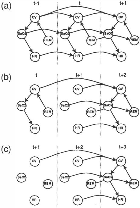
For a one-step ahead forecast, DYNEMO generates fore­ casts by performing probabilistic inference on BN�;t. The posterior marginal distributions of the leading­ slice nodes are the forecast distributions. For example, the network in Figure la depicts the topology of the sleep-apnea DNM and of the corresponding BN�;1.

For a k-step ahead forecast, DYNEMO recursively gen­ erates BN�-;2, BN�-;3 , ... , BN�;k. To generate BN�;i,

DYNEMO remo _v es arcs from nodes in BN�;i - 1 according to the followmg rule:

If node Xt is uninstantiated in BN�;i-1 ? then render node Xt-1 a prior node in BN�;' with a prior distribution equal to the posterior marginal forecast of Xt in BN�;i - 1 .

These structural changes may disconnect the network. For example, the DNM of Figure 1a generates the BN�-;2 in Figure 1b; BN�-;2 is then used to generate the disconnected network BN�-;3 in Figure 1c. Higher­ order forecasts are generated by performing probabilis­ tic inference on the respective BN�+i, after instantiat­ ing the appropriate temporal evide�ce.

Let I be the highest-order lag of a node in the leading time slice of a D NM. Note that there will be min (I, k) unique BN�+i that must be constructed to generate k-step ahead forecasts.

DYNEMO provides both exact (Lauritzen-Spiegelhalter) and approximate (BN-RAS [7]) probabilistic inference for computing forecast distributions. Exact inference is more efficient than approximate inference when time series contain few missing values, in which case the BN�;i are predominantly instantiated.

To update the DNM parameters, DYNEMO instantiates the leading-slice model variables in BN�-; 1 with freshly observed evidence and computes new parameter values using the update method specified by the user (see Section 3.3).

' To visualize the results of forecasting, DYNEMO outputs expected values of the k-step ahead forecasts for graph­ ical analysis within Mathematica[25]. Mathematica plots observed data versus forecast data and computes and plots the sum of the squares of the residuals (see Section 5).

5 THE SLEEP-APNEA FORECASTING PROBLEM

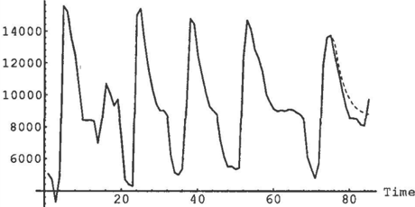
In 1991, the Santa Fe Institute organized a time-series forecasting competition [30]; one of the databases made available in that competition was a multivari­ ate data set of 34,000 recordings, sampled at 2 Hz, of heart rate (HR), chest volume (CV), blood oxygen con­ centration (Sa02), and sleep state (REM). The data were collected from a patient suffering from sleep ap­ nea in the sleep laboratory of the Beth Israel Hospital in Boston, Massachusetts.

5.1 SLEEP APNEA

Sleep apnea is a serious and prevalent medical condi­ tion, characterized by periods during which a patient takes a few quick breaths and then stops breathing for up to 45 seconds. This pattern is repeated as many as 200 to 400 times during six to eight hours of sleep.

The main clinical consequence of sleep apnea is exces­ sive daytime sleepiness related to the fragmentation of sleep and the effects of hypoxemia on cerebral func­ tion. Thus, for example, patients with severe obstruc­ tive sleep apnea are involved in automobile accidents two to three times more often than the general popu­ lation. In addition to daytime sleepiness, studies im­ plicate sleep apnea in systemic hypertension, cardiac arrhythmias, myocardial infarctions, and sudden car­ diac death [19].

In a population-based sample of working men and women 30 to 60 years of age, Young et al. [32] show that 4 percent of women and 9 percent of men in this group have 15 or more episodes of sleep apnea per hour of sleep. In 1988, Congress established the National Commission on Sleep Disorders Research "to develop a long-range plan for the use and organization of na­ tional resources to deal effectively with sleep disorders research and medicine" [24]. A time-series analysis of sleep apnea variables provides a model for predicting the onset of sleep apnea before it occurs. The analysis is also valuable because it sheds light on the physiolog­ ical events prior to the onset and on the relationships between the evolutions of the variables.

5.2 MODEL STRUCTURE

The sleep-apnea data set contains three continuous variables (HR, CV, Sa02) and one discrete variable (REM). The CV and Sa02 sensors were known to drift slowly over time, and were occasionally rescaled by a technician; hence, their calibrations were known not to be constant over the entire data set.

To discretize the continuous variables, we used Knowl­ edgeSeeker [11], a clustering program based on au­ tomatic interaction detection [21]. KnowledgeSeeker produced 7-valued discretizations for each continuous variable.

We then used DYNEMO to generate probable DNM structures from a subset of the database, using the modified K2 metric and the partial ordering imposed by the temporal nature of the model variables. We then refined the model with knowledge of cardiovascu­ lar and respiratory physiology, during the process of model fitting and diagnostic checking. The final DNM is shown in Figure la. Note that the model has an irregular structure and that CVt + 1 depends not only on CVt, but also on CYt-1· DYNEMO can generate and forecast DNMs with highly irregular structures and noncontemporaneous dependencies that span multiple time points.

5.3 MODEL FORECASTS

We present the results of an experiment using the DNM from Section 5.2. We generated the apnea DNM using the first 27,000 time points from the data set, and then used the model to generate the one­ step through ten-step-ahead forecasts for the remain-

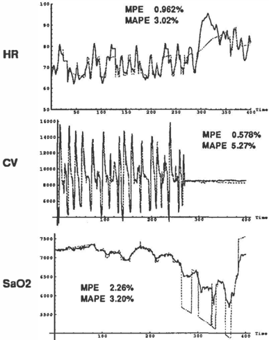
ing 7,000 time points. Figure 2 depicts one-step ahead forecasts for HR, CV, and Sa02, respectively, for the interval t = [27001, 27400].

To analyze our results, we use several measures from statistical forecasting. The prediction error at time t is the difference between the observation at time t, Ot, and the prediction for time t, Pt. The percent prediction error (PPE} at timet is given by 0 '0,P' x 100. The mean prediction error (MPE) is given by .l. "\'N 01- P 1 N L.... t =l 01 ·

The MPE is the sum of the prediction errors normal­ ized by the level of the series measured. Thus, we can compare the MPE between different time series. The MPE measures the bias of the model predictions, and therefore, it measures how closely the predictions follow the level of the time series. Statisticians seek values of the MPE that are zero; deviations from zero indicate model bias.

The mean absolute prediction error (MAPE) is given by /:t E�1 1°'0,Ptl. The MAPE measures the dis­ persion of the model predictions. Thus, the MAPE measures how well the predictions capture the turn­ ing points in the time series. Whereas the MPE is near zero when the prediction errors cancel, the MAPE may be quite large if the prediction errors are large. Figure 2 gives the MPE and MAPE for HR, CV, and

Sa02 for the one-step-ahead predictions in the interval 27001 to 27400.

Notice that in Figure 2, an episode of sleep apnea starts at time 270, corresponding to time point 27270. During the apneic episode, the chest volume is con­ stant, as we expect since the patient has stopped breathing. The blood oxygen saturation, measured by the Sa02, drops during the the apneic period because the patient is not breathing. Also during the apneic period, we observe an increase in the baseline heart rate.

Thus, the three time-series are cross-correlated since concomitant level changes occur during apneic episodes. We also observe concomitant changes dur­ ing breathing: inspiration (increasing chest volume) causes a decrease in heart rate. This phenomenon is known as sinus arrhythmia. Thus, the time series also have cross-correlated cyclicities.

Figure 2 presents the MPE and MAPEs for the one­ step ahead forecasts for HR, CV, and Sa02. Because the MPE and MAPEs are dimensionless measures, we can compare their values between different time series. We conclude that there was negligible bias in the HR and CV forecasts. The Sa02 forecasts had a larger bias but the bias is well within the acceptable limit. The MAPE measures the dispersion of the forecasts. The CV forecasts had the largest dispersion, even though of the three forecasted variables, the CV forecasts fol­ lowed the time-series values closest. The nature of the CV time series explains the wide dispersion of the CV forecasts. The CV time series has rapid, large­ amplitude oscillations, which magnify the prediction errors, and therefore, increase the dispersion.

The HR forecasts smooth the real time series: the fore­ cast series truncates peaks and smooths out troughs. However, the forecasts capture turning points in the time series and closely follow the level of the series. The smoothing behavior reflects the forecast's inertia to adapt to the apneic episode, apparent during the time interval between 300 and 350. The CV forecasts follow tightly the real data, capturing all the turning points. The Sa02 forecasts follow the series closely un­ til the apneic episode. At this point, although the fore­ casts respond to the turning points in the series, the trough levels of the time series were poorly modeled by the forecast series. A plot of the prediction errors (not shown) confirms that trough levels are poorly mo � e � ed during the apneic episode: we observe large positive deviations in comparison to the negligible and unbi­ ased prediction errors that precede the apneic episode. The discretization of the time series in the range of the apneic episode, 5700-6500, is too coarse for the forecast values to accurately capture the predictions.

In Figure 3, we show one through ten step-ahead fore­ casts starting at time 27075. The initial few forecasts follow the real data closely. The prediction error in­ creases as we forecast further into the future.

6 CONCLUSIONS

We have been motivated by the need for a time-series model· that can be applied to the dynamic domains encountered in complex probabilistic-reasoning appli­ cations. DNMs are ideally suited for time-series mod­ eling, forecasting, simulation, and control in domains for which prior knowledge is available about the dy­ namic forces and relations at work, but is sufficiently complex to preclude a complete specification. These are the domains that we face in probabilistic-reasoning applications.

From the perspective of AI, DNMs inherit the rep­ resentational virtues of belief networks and influence diagrams. DNMs (1) are explicative models of the do­ main, as opposed to merely descriptive ones; (2) fa­ cilitate the knowledge-engineering tasks of knowledge acquisition and representation; (3) can make norma­ tive prescriptions; and ( 4) are amenable to a variety of efficient inference algorithms. On the other hand, there is too much uncertainty in the time evolution of a dynamic domain for conventional belief-network mod­ els to be of value. This uncertainty arises from varia­ tions in unmodeled exogenous forces, which are typi­ cally too numerous, too difficult, or too obscure to be modeled realistically. If we specify unique conditional­ probability distributions to model the dynamic behav­ ior of a complex domain we must sum over all possible states of the unmodeled exogenous influences. Thus, we increase substantially the variance of the condi­ tional probabilities, and therefore, decrease the utility of the model.

From the perspective of time-series analysis, DNMs allow (1) measurement and system equations to be highly nonlinear or specified nonfunctionally; (2) lag influences to be modeled by system equations that are higher-order Markov processes; (3) the specifica- tion of disturbance distributions in either functional or table form; and ( 4) the specification of contempo­ raneous influences of any nature. Furthermore, prob­ abilistic inference in DNMs is akin to Kalman filter­ ing. Thus, DNMs extend state-space models in every respect. But unlike the problems of tractability and accuracy that we encounter in using Kalman filters with nonnormally distributed disturbances, inference in DNMs is amenable to a number of efficient inference algorithms and to results on the second-order prob­ ability distribution of the estimate. By making use of the conditional-independence statements explicit in a belief network, inference algorithms achieve greater efficiency and superior accuracy as compared to all­ purpose Monte Carlo algorithms used in nonnormal state-space models.

DNMs extend classical time-series analysis and pro­ vide an expressive methodology for ongoing research on temporal probabilistic reasoning. Current research on DNMs includes the convergence analysis of model update methods, the construction of models in the fre­ quency domain, and the development of discrete-event simulation and temporal decision models.

Acknowledgments

We are grateful to Eric Horvitz for sharing with us his insights into the subject of this paper. This work was supported by the National Science Foundation under grant IRI-9108385, by Rockwell International Science Center IR&D funds, and by the Stanford University CAMIS project under grant IP41LM05305 from the National Library of Medicine of the N ational Institutes of Health.

References

1. B. Abraham and J. Ledolter. Statistical Methods for Forecasting. Wiley, New York, 1983.
2. B. Abramson. ARC01: An application of be­ lief networks to the oil market. In Proceedings of the Seventh Conference on Uncertainty in Ar­ tificial Intelligence, pages 1-8, Los Angeles, CA, July 1991. Association for Uncertainty in Artifi­ cial Intelligence.
3. F. Bacchus. Representing and Reasoning with Probabilistic Knowledge: A Logical Approach to Probabilities. MIT Press, Cambridge, MA, 1990.
4. C. Berzuini, R. Bellazzi, and S. Quaglini. Tem­ poral reasoning with probabilities. In Proceedings of the 1989 Workshop on Uncertainty in Artificial Intelligence, pages 14-21, Windsor, Ontario, July 1989. Association for Uncertainty in Artificial In­ telligence.
5. R. G. Brown. Smoothing, Forecasting and Predic­ tion. Prentice-Hall, Englewood Cliffs, NJ, 1963.

• [6) G. Cooper and E. Herskovits. A Bayesian method for the induction of probabilistic networks from data. Machine Learning, 9:309-347, 1992.
• [7) P. Dagum and R.M. Chavez. Approximating probabilistic inference in Bayesian belief net­ works. Pattern Analysis and Machine Intelli­ gence, 15(3):246-255, 1993.
• [8) P. Dagum and A. Galper. Additive belief net­ work models. In Proceedings of the Ninth Con­ ference on Uncertainty in Artificial Intelligence, Washington, DC, July 1993. Association for Un­ certainty in Artificial Intelligence.
• [9) P. Dagum, A. Galper, and E. Horvitz. Dynamic network models for forecasting. In Proceedings of the Eighth Workshop on Uncertainty in Artifi­ cial Intelligence, pages 41-48, Stanford, CA, July 1992. American Association for Artificial Intelli­ gence.
• [10) P. Dagum, A. Galper, and E. Horvitz. Dynamic network models for temporal probabilistic rea­ soning. Technical Report KSL-91-64, Section on Medical Informatics, Stanford University, Stan­ ford, CA, 1992. Under review for Pattern Analy­ sis and Machine Intelligence.
• [11) Barry de Ville. Applying statistical knowledge to database analysis and knowledge base construc­ tion. KnowledgeWorks Research Systems Ltd., Ottawa, Canada, 1990.
• [12) T. Dean and K. Kanazawa. Probabilistic causal reasoning. In Proceedings of the Fourth Workshop on Uncertainty in Artificial Intelligence, pages 73-80, Minneapolis, MN, August 1988. American Association for Artificial Intelligence.
• [13) T. Dean and K. Kanazawa. A model for reasoning about persistence and causation. Computational Intelligence, 5:142-150, 1989.
• [14) T. L. Dean and M. P. Wellman. Planning and Control. Morgan Kaufmann Publishers, San Ma­ teo, CA, 1991.
• [15) J. C. Spall (Eel.). Bayesian Analysis of Time Se­ ries and Dynamic Models. Marcel Dekker, New York, 1988.
• [16) J. Y. Halpern. An analysis of first-order logics of probability. In Proceedings of the Eleventh In­ ternational Joint Conference on Artificial Intelli­ gence, pages 1375-1381, 1989.
• [17) A.C. Harvey. Forecasting, Structural Time Series Models, and the J( alman Filter. Cambridge U ni­ versity Press, New York, 1990.
• [18) E. Herskovits. Computer-based Construction of Probabilistic Networks. PhD thesis, Program in Medical Information Sciences, Stanford Univer­ sity, Stanford, CA, 1991.
• (19] J. W. Shepard Jr. Hypertension, cardiac arrhyth­ mias, myocardial infarction, and stroke in rela­ tion to obstructive sleep apnea. Clinics in Chest Medicine, 13:437-458, 1992.
• [20) K. Kanazawa. A logic and time nets for proba­ bilistic inference. In Proceedings of the Ninth Na­ tional Conference on Artificial Intelligence, pages 360-365. American Association for Artificial In­ telligence, July 1991.
• G. V. Kass. An exploratory technique for inves­ tigating large quantities of categorical data. Ap­ plied Statistics, 29:119-127, 1980.
• [22) C.R. Kenley. Influence diagram models with continuous variables. Technical Report LMSC­ D067192, Astronautics Division, Lockheed Mis­ siles & Space Company, Sunnyvale, CA, June 1986.
• [23) U. Kjaerulff. A computational scheme for reason­ ing in dynamic probabilistic networks. In Proceed­ ings of the Eighth Conference on Uncertainty in Artificial Intelligence, Stanford, CA, 1992. Asso­ ciation for Uncertainty in Artificial Intelligence.
• [24) National Commission on Sleep Disorders Re­ search. Wake up America: a national sleep alert. Government Printing Office, 1993.
• Wolfram Research. Mathematica 2.0. Addison­ Wesley, Redwood City, CA, 1991.
• Y. Shoham. Reasoning About Change: Time and Causation from the Standpoint of Artificial Intel­ ligence. MIT Press, Cambridge, MA, 1988.
• (27] Y. Shoham and N. Goyal. Temporal reasoning in artificial intelligence. In Exploring Artificial Intelligence. Morgan Kaufmann, San Mateo, CA, 1988.
• [28) J. Tatman. Decision Processes in Influence Dia­ grams: Formulation and Analysis. PhD thesis, Department of Engineering-Economic Systems, Stanford University, Stanford, CA, 1985.
• J. Tatman and R. Shachter. Dynamic program­ ming and influence diagrams. IEEE Transactions on Systems, Man, and Cybernetices, 20:365-379, 1990.
• (30] A. Weigend and N. Gershenfeld. Time-series com­ petition. In M. Casdagli and S. Eubank, editors, Nonlinear Modeling and Forecasting: Proceedings Volume XII, Santa Fe Institute Studies in the Sci­ ences of Complexity, page 17. Santa Fe Institute, Addison-Wesley, September 1990.
• (31] M. West and J. Harrison. Bayesian Forecasting and Dynamic Models. Springer-Verlag, New York, 1989.
• (32] T. Young, M. Palta, J. Dempsey, J. Skatrud, S. Weber, and S. Baclr. The occurrence of sleep­ clisorclerecl breathing among middle-aged adults. New England Journal of Medicine, 328:12301235, 1993.