Fraud/Uncollectible Debt Detection Using a Bayesian Network Based Learning System: A Rare Binary Outcome with Mixed Data Structures

Kazuo J, Ezawa

Room 7E-523

Til Schuermann

Room 7E-530

[email protected] til@ ulysses.att.com

AT&T Bell Laboratories 600 Mountain A venue Murray Hill, N. J. 07974

Abstract

TI1e fraud/uncollectible debt1 problem in the telecommunications industry presents two technical challenges: the detection and the treaunent of the account given the detection. In this paper, we focus on the first problem of detection using Bayeshm network models, and we briefly discuss U1e application of a nonnative expert system for U1e treatment at tl1e end. We apply Bayesian network models to the problem of fraud/uncollectible debt detection for telecommunication services. In addition to being quite successful at predicting rare event outcomes, it is able to handle a mixture of categorical and continuous data. We present a performance comparison using linear and non­ linear discriminant analysis, classification and regression trees, and Bayesian network models.

1 INTRODUCTION

Every year, the telecommunications industry incurs several billion dollars in uncollectible revenue, the vast majority of which ts in the fonn of net bad debt (NBD).1 In this competitive industry, cost efficiency is panunount for success and survival, and NBD is a prime target for high-impact cost cutting. We seek to provide the business wiU1 two tools: one which will surpass existing detection meU10ds, and a second which will provide recommendations of how to handle t11e customers identitied by U1e tirst. In this paper we present the Advanced Pattern Recognition and Identitication (APRI) system, which is a Bayesirm network supervised machine learning system, and compare its performance to existing methods such as statistical discriminant analysis and classitication and regression trees (CART) [Breiman, Friedman, Olshen and Stone, 1984].

1 Uncollectible debt is the sum of NBD. direct adjustments, coin shot1ages and unbillable messages.

As is no surprise, the NBD detection problem is a difticult one. We are essentially trying to find a small but valuable needle in a rather large haystack. For one, we are dealing with a binary outcome (a call or a customer is eiU1er .. good" or "bad'' from a collections perspective), where t11e outcome of interest occurs quite rarely: 1 -2 % of the time, in fact. 2 Second, falsely classifying a good customer as bad could have dire consequences: we could lose such a customer. APRI allows t11e detection and identitication of potential cru1didates: how to handle t11em is another matter. For tl1is we are developing Nonnative Expert System Development Tool (NESDT) to provide intelligent decision support for account treaunent recommendation for such a candidate.

Finally, modeling is made still more difficult because t11e data at our disposal is boU1 discrete and continuous in nature. Exmnples would be t11e total monthly bill of a customer (in dollars, which is continuous) and t11e area code of residence (which is categorical or discrete). There are metl10ds designed to handle either one or t11e ot11er kind of data effectively, but none deal wiU1 a mixed situation satisfactorily. In addition to U1e data characteristics which make modeling difficult, the sheer size of U1e data sets under consideration, while large by research standards (4-6 million records and 600-800 million bytes), are small by telecommunications industry standards. Some learning metlwds simply cannot hope to process t11is much data in a timely manner.

We will be comparing our APRI system to discriminant ru1alysis and CART 3 . In addition we attempted a comparison wit11 t11e classitication tree met11od of C4.5 [Quinlan, 1993] but were unable to complete a run. TI1e

2 We have selected our data segment carefully so that our data set proportions are more favorable for learning. For this paper we have an empirical uncollectible rate of 8-10%.

3 We are using a software internally developed and implemented based on "CART' m�thodology.

C4.5 implementation is simply unable to handle data sets as large as our. However, we have an implementation of CART that is able to handle data sets of this size, although we encountered other problems. In discriminant analysis we estimate a linear or quadratic combination of explanatory variables to define a discriminant function which classifies each member of the sample into one of two groups. Discriminant rumlysis is a popular statistical method witl1 specific underlying distributional assumptions (such as nonnality) used for classification when t11e data available are mostly continuous and when the populations are relatively balanced, something which is clearly not the case here. By contrast, Bayesian classifiers in general, and APRI in particular, make no distributional assumptions. APRI first selects key variables and then computes the prior probability distribution based on the training set for each selected variable. As new infonnation or evidence arrives, we update t11e prior probability to compute a posterior. Therefore as we receive more information/evidence, we can fonn a more accurate profile of t11at particular customer or call.

Classification trees, when used for classification, are best when the feature set is mostly categorical and when, as with discriminant ru1alysis, t11e population groups are relatively balanced. Note however t11atCART also has a "regression" component, but in our ru1alysis we restricted ourselves to the classification tree side.

2 DATA AND ISSUES

The met11odology which we describe is designed to address a large class of problems. Our motivation is largely practical as opposed to purely t11eoretical. We are faced with four major issues.

1. There are two populations; however, one has only a very low probability of being observed (-8-10% in our concentrated sample, < 2% in population) and accounts wit11in t11e same population are not homogeneous; there may be many undefined sub-groups in each population.
2. The predictors are of mixed data types: some are categorical, some continuous. Their characteristics are: i) The continuous variables can not be assumed to be normally distributed. ii) The categorical variables are themselves a mixed bag. Some have binary or trinary outcomes and could t11erefore be easily handled wit11 dummy variables, ot11ers have many outcomes (e.g. 44, 130 or 1000+) and recoding t11em into binary outcome variables can be quite inefficient. Moreover, none of t11e categorical variables are ordered, precluding t11e use of a latent variable model.

Statistical discriminant analysis procedures for mixed variable cases do exist [see Krzanowski, 1980, Knoke, 1982, and Krzanowski, 1983]. However, they presume t11at none of t11e population groups is very small relative to t11e others (i.e. there are no "rare events"), and the continuous variables, conditioned on tl1e outcome of a categorical variable, are normally distributed.

Clearly, bot11 of these assumptions are violated by our problem. If not, then for many mixed variable cases, statistical dist..1.nce metrics such as Mal1alanobis distance are preferred to information theoretic metrics such as Kullback-Leibler distance (also known as relative entropy) [Krzanowski, 1983].4 While classical discriminant analysis based on Mahalanobis distance metrics has been shown to be robust to departures from nonnality, our application brings with it too many violations of t11e classical assumptions. In preliminary analysis we have found discriminant analysis to perform poorly when compared to our new approach. The departure from normality together witl1 the mixture of categorical and continuous data immediately suggests a non-parametric, or distribution-free approach.

1. For misclassification cost, t11e issue is very complex, not const..'lnt per class. Misclassification cost depends on t11e account treatment decision, tl1e account itself, the customer's reaction, federal and state legal and regulatory constraints, and ot11er factors.

Let us consider t11e issue of misclassification costs more carefully. In our telecommunications applications, it is highly undesirable from a business perspective to misclassify a good customer as bad. The costs associated wit11 t11is event are different for every customer: it will depend on t11e expected lifespan of the customer with the company (a customer who would ot11erwise have remained with AT&T for two years is clearly more costly to lose t11an one who would have only remained for two mont11s) and on t11e potential action taken wit11 such a falsely identified customer (Do you shut him down? Do you call him? Do you send a letter?). The best option in fact could be "do not11ing". This is a complex decision process wit11 much uncertainty and would be best handled wit11 t11e aid of NESDT, a decision t11eoretic normative expert system. Thus each account (or case) has a different misclassification cost associated with it, and the cost is in tum conditional on t11e action taken subsequent to identification and on t11e customer's reaction.

4 All methods have the same first order asymptotic behavior. However, under the assumptions of normality, maximum likelihood achieves second order asymptotic superiority and disciminant analysis using Mahalanobis distance is optimal.

This is one of tl1e key issues tl1at led to t11e separation of fraud/uncollectible detection and account treaunent. APRI focuses on detection, and passes tl1e fraud/ uncollectible probabilities to NESDT for account treatment recommendations. The expected misclassification cost for each account is implicitly computed in tl1e NESDT using information such as tl1e above factors, plus otl1er factors (e.g., t11e expected account life, tl1e account profitability, etc .. ). We believe it is improper to artificially bias t11e fraud/uncollectibe probabilities at t11e detection stage by imposing arbitrary misclassification cost.

4) Aside from tl1e very nature of t11e data, its sheer size poses a problem as well. In our telecommunications network, a couple hundred million calls arc placed daily. Each call provides us a couple hundred bytes of infonnation. Hence we accumulate 40-50 giga-bytes (GB) of infonnation daily. The data sets under <malysis (a more detailed description is contained in Section 4) range anywhere from 8 mega-bytes (MB) to nearly 800 MB in size. Still, 800 MB is a tiny fraction of daily call detail infonnation. In fact, since tl1is application is in t11e telecommunication sector, any implementation is likely to impose similar data requirements on <my modeling metl10d. Hence t11e metl10d, or more importrullly t11e algorithm or software, must be able to cope witll data sets of this magnitude. It is indeed a nontrivial accomplishment t11at APRI is able to handle this with relative ease.

3 CLASSIFICATION METHODS

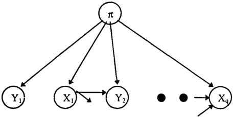
Let us consider the case of two populations, 1t1 and 1t2, with a sample of n1 and n2 from each. We have two sets of characteristics: 1) Let Y be a c-lengt11 vector of continuous variables. 2) Let X be a q-lcngth vector of discrete or categorical variables.

The classification problem can be described by the joint probability of classes/population [7t] and t11eir attributes [Y,X], i.e., Pr{7t,Y,X}. The classitication of the classes is based on tl1e conditional probability of Pr{7tiY,X}. The various metl1ods differ principally in the way tlmt the conditional probability of the classes 1t given the data is computed.

3.1 DISCRIMINANT ANALYSIS

Classical discriminant analysis assumes that the explanatory variables are jointly nonnally distributed, and that Pr{1tiY,X} can be generated from a discriminant function. Under tl1is assumption, if t11e covariance matrices of tl1e two populations are equal, tl1e optimal classification rule is tl1e linear discriminant function. If we for the moment only consider the continuous variables Y, tl1e sample linear discriminant function can be expressed as:

where Y i are tl1e san1ple mean vectors and S is the pooled sample covariance matrix. A new observation Yo is then classified into 1t2 according to the rule:

where c is chosen according to objectives of the problem at hand. It turns out tl1at tl1e classitication rule which minimi,es ilie of misc : , ::: ob.Uned by Jetting

If the covariance matrices of the two populations are unequal, then we may use quadratic discriminant ru1alysis which t..'lkes explicit account of the differing covariance matrices, S1 and Sz. Again considering only the continuous variables for the moment, an observation Y would be classitied into 1t1 if

It comes as no surprise that, as the divergence between the two populations, measured by ISd and IS21, decreases, the efficiency gain of using t11e quadratic instead of linear discriminant model decreases as well.

In nonparametric discriminant analysis, the conditional density of the class given tl1e data is estimated directly, say via a kernel density algorithm. As the dimensionality of t11e feature set increases, the computational intensity increases dnuuatically. This is another manifestation of tl1e well-known "curse of dimensionality", and in practice nonparrunetric discriminant analysis is useful for no more t11an t11ree or four features or characteristics.

3.2 THE BAYESIAN NETWORK APPROACH

In theory, a "Bayesian Classifier" [Fukunaga, 1990] provides optimal classification perfommnce, but in practice so far it has been considered impractical due to enormous data processing requirements. Recent advances in evidence propagation algorit11ms [Shachter 1989, Lauritzen 1988, Jenson 1990, Ezawa 1994) as well as advances in computer hardware allow us to explore tl1is Bayesian classifier in tl1e Bayesian network form [Cheeseman 1 988, Herskovits 1990, Cooper 1992, Langley 1994, Provan 1995].

3.2.1 The Bayesian Network

To assess the conditional probability of Pr{rriY,X} of classes directly is often infeasible due to computational resource limitations. TI1erefore, we tirst assess the conditional probability of the attributes given the classes, Pr{Y,XIrr}, and t11e unconditional probability of the classes, Pr{ rr }, using a preclassitied training data set.

Figure 1 shows an exmnple of a model where Pr{Y,XIrr} is furtller factorized to attribute level relationships Pr{Y 1 11t} * P{Y 2 1 X�orr} * ... * Pr{XqiY;, .. ,rr}.

Once we assess tl1e Pr{Y,XIrr}, using Bayes rule, we compute t11e conditional probability Pr{ rriY,X} with observed values of Y, X.

3.2.2 The association metric: entropy

TI1e Advm1ced Pattern Recognition & Identification (APRI) system we developed is a Bayesi<Ul network-based supervised machine learning system resting on the above principle. We employ t11e entropy-based concept of mutual information to perfom1 dependency selection. It first selects a set of variables and t11en selects a set of dependency muong t11e selected variables using heuristically selected cumulative entropy thresholds. We settled on tl1is approach to reduce the training time with special attention on repeated reading of training dataset as opposed to t11e methods used in [Herskovits 1990, Cooper 1992, Quinlan 1993, Provan 1995] where one variable or one segmentation of a variable is selected at a time.

Mutual information is defined for a pair of discrete random variables xj, xj as

Mutual infonnation is used to rank population characteristics (or field nodes, to use the language of APRI) by how well tl1ey can discriminate between the two (or more) groups. It finds dependencies between

U1ese field nodes as well as to create a conditionally dependent model. Note t11at t11e mutual information metric is used only to determine model size and structure: how many field nodes to keep and which field to field node dependencies to allow for a conditionally dependent model. This is analogous in statistical regression analysis to variable selection for model specitication.

Finding the optimal structure of a Bayesian Network is an NP hard problem, and we are tl1erefore forced to engage in a heuristic search for tl1e structure based on mutual infonnation.

TI1e first step of the training process for APRI is to create a schema tile, which provides infonnation how each variables are treated, feature selection information, variable definition (e.g.. continuous & and discrete, discretization met110ds or kemel density for continuous variables, etc.), cumulative entropy t11resholds (percentage of total cumulative entropy), one for prime to field Tpr (0 :s; Tpr :s; 1), tl1e ot11er for field to field Ttr (0 :s; T tr :s; I), and moving window size (i.e., whetl1er it uses a single record or multiple records at a time), etc ..

APR/ Training Algorithm:

• *I Input schema file and training dataset */
• a) if rr is continuous, compute class outcome set first b) compute outcome sets for X; Vi= l, ... ,q possible attribute variables, and rr (discrete classes).
• a) compute all pairwise mutual information between prime and each field node Ml(rr;X;) Vi= 1, ... ,q possible attribute variables
• select field variables in descending order until Tpr is reached
• a) compute all pairwise mutual infonnation between field nodes conditional on tl1e prime node Ml(Xi;X;Irr) V j 1o i.
• select field to field dependencies in descending order until T tr is reached
• compute P{X;IC(X;)} and P{rr} where C(X;) represents parents of X; including rr.

First (as a part of step 1), in a continuous classification task, APR! reads tl1e training dataset to discretize or to estimate tl1e kemel density of t11e classes. (TI1is first step is unnecessary in discrete classification tasks.) Second (as t11e ot11er part of step 1 ), it reads t11e training dataset to detine U1e outcomes of each variable. It also discretizes continuous outcomes using entropy measures or estimates t11e kernel for example. On t11e t11ird pass (step 2) it selects the variables to keep. On the fourth (step 3), it selects t11e dependencies among t11e previously selected variables. Finally (step 4), tl1e dataset is read again to

obtain the conditional probability distributions for the selected variables given t11e chosen dependencies. APRI performs better witl1 higher Tpr and Ttl tluesholds, but it is constrained by t11e computational environment (e.g., in tlle 32 bit operating system, a single model size is restricted to 2GB.)

We did not take t11e approach of [Herskovits 1990, Cooper 1992, Heckenmm 1994, Provru1 1995] to compute the joint probabilities P{B8,D}, where Bs is a Bayesian network structure, and D a dataset. First of all, our dataset violates most of the basic assumptions made for this approach; i.e, 1) it contains a mixture of categorical and continuous variables, 2) the records are not necessarily independent e.g., we have a sequence of calls from t11e same customer, and 3) we have many missing values. Secondly, the creation of an index tree 5 itself could be a problem. Just two variables with 1,000+ outcomes (e.g., originating and terminating cities) could create a link list of 1,000,000 cells. A few more variables like tl1is makes it infeasible to construct and store the index tree, given the current computing environment. Thirdly, even if we succeed in creating the index tree 6 , we will face a run time problem. In order to create a model, t11e training dataset needs to be read n ( u + 1) times, where n is a number of variables and 11 is tl1e maximum number of parents allowed. If you have a 4 million record training dataset with 33 variables (discussed later in Section 4.2), we would need to read tl1e data 66 times witl1 u = 1. In the case of discrete outcome classification, APRI needs to read tl1e data set only four times regardless of tl1e number of attributes or associated outcomes.

Lastly, even if we were to build an optimal Bayesian network model, it would become obsolete quite rapidly. TI1e fraud/uncollectible debt problem environment is not static, but dynrunic. In addition to tl1e time related dynamics, more importantly, the detection model we create itself directly impacts the fraud/uncollectible problem environment of tomorrow. The better tl1e model, the more quickly it becomes obsolete. TI1e more successful we are in detecting and treating ti1e fraud/uncollectible accounts or calls, the fewer accounts or calls will fit ti1e existing model for future detection. l11e fraud/uncollectible problem simply evolves into a different shape and fonn and adjusts to tl1e new environment. We may in fact not be able to find a "gold standard" Bayesiru1 network structure. TI1erefore, given ti1at the model will need to be retrained oflen, we put

5 See Cooper ( 1 992 ) . pp. 326-327.

6 Since our dataset is large. to obtain a value in the index tree, it needs to access the dataset itself on a hard disk.

more emphasis on tile ability to create a good model in a reasonable time using a very large dataset.

Avoidance of probability of 1 ("Pruning"): A particularly useful feature of APRI is its ability of avoiding ti1e degenemcy of a probability at t11e tail end of the evidence propagation operation in tile classification process. This feature allows us to separate tile impact of ti1e model's complexity from pure overfitting. l11e feature is simple. We skip tile field node which causes P{ ·} = 1 in tl1e classification process as we would if we had missing infonnation (or missing observation) for ti1at field node. It is essentially tile "pruning" of t11e tail-end attributes in tile process of classification. Note mat tlliS effect of "pruning" is not explicitly observable on the network itself. It is implicitly hidden in tl1e data structure under each field node.

Moving windows: APRI can model record dependency which is often manifested as tile passage of time. It can create a model based on a set of variables over a specific lengti1 of a sequence. For example, tile call detail dataset contains tl1e time related information. APRI can exploit tile sequence of calls to create a model. Otl1ers can do so only with extensive dataset refonnatting 7 ·

3.3 OTHER METHODS: C4.5 AND CART

A well-known implementation of tile entropy based metric is ti1e machine learning program C4.5 by [Quinlan 1993]. In fact, C4.5 is a natural competitor to APRI because of tl1is. 8 Similar to CART, C4.5 progressively splits the data set under investigation into subsets on increasing homogeneity. Quinlan noted tl1at his entropy bw;ed gain criterion, used to determine such splits, exhibits a strong bias in favor of tests witi1 many outcomes. He suggests scaling tl1e gain criterion by a measure of marginal infonnation gain from tile split under consideration 9 . We are faced with a similar problem where nodes witi1 many outcomes yield artificially high mutual infonnation wit11 respect to the prime node (classes) and oti1er field nodes (under a conditionally dependent model). We are currently experimenting witi1 several heuristic scaling or deflating factors.

C4.5 failed in building a model for our data set because of its sheer size. This is particularly disappointing because we have used only summary data for ti1e test.

7 When faced with a large dataset like ours, duplication and reformatting of the dataset should be minimized to reduce the training time and storage space.

8 For an initial comparison to standard data sets. see [Ezawa and

Schuermann, 19941.

9 See Quinlan (1993). p.23.

The final business application will require call detail level data which will increase the data set size up to 100 fold. C4.5 in its present fonn is therefore not operationalizable for this application.

The classification and regression tree (CART) approach of [Breiman, Friedman, Olshen and Stone 1984] was originally developed because of the shortcomings of discriminant analysis when faced wiU1 mostly categorical data. 10 In theory CART accepts any distance or deviation metric, but U1e algoriUm1 we used, based on the S software, employed the likelihood metric. u [Rao 1963] has provided results U1at demonstrate first-order asymptotic equivalence between models estimated by different metrics such as likelihood, entropy or minimum chi-square.

4 APPLICATION TO UNCOLLECTIBLE DETECTION

We now make a direct comparison of the performance of the Ulree metl1ods, where the benchmark is the "Do NoU1ing" strategy. At the very least, �my metlwd should be able to beat this alternative. We have concentrated the sample along a few dimensions for several reasons, mainly because from a business perspective U1e problem is interesting (at U1e moment) only for certain customer segments. In U1is paper we present the results of comparison using account summary dat<t (40K 80K records, 8 - 12 million bytes). ·n1en we show preliminary results from APRI for out-of-sample prediction using detailed account activity dataset (4-6 million records, 600-800 million bytes of data).

For practical implementation, we need to train U1e model for a particular period and test it on a subsequent period of data. In this sense out-of sample prediction is not witl1 a typical hold-out sample of the srune period but a full set from a subsequent period. This makes the testing of the models harder but more realistic.

When considering goodness of fit, U1e conventional metric is the correct classification rate. Our concerns are somewhat different. We are principally worried about the number of customers classitied as uncollectible, be they actually. good or bad. Thus a metlwd which classifies nearly everyone as collectible, yielding a respectable correct classitication rate overall, will be

10 See Breiman et al. (1984), pp. 15-16.

11 Since the S version of CART is limited to small data sets. a nomrivial hurdle for this application, we made use of a modified version developed at Bell Laboratories. This C-hased version can accept very large data s e ts and is otherwise identical to its S cousin.

useless for us; it is litUe different from U1e status quo of "Do NoU1ing".

In U1e Tables 1 and 2, U1e numbers in square bmckets indicate the number of customer accounts for Ulat cell. We include U1is infonnation in addition to U1e classification percentages to highlight U1at even if Ule correct classification percentages are promising, Ule absolute numbers may not be simply because U1e populations are so unbalanced. FurU1ennore, beneaUl each table we have predicted collectible to uncollectible odds. This is useful because from an operational perspective, we are interested in just what proportion of U1e predicted population is in each group. Since Ule "Do NoU1ing" alternative makes no uncollectible predictions at all, we want to understand how any given model perfonns relative to U1is option, which if all models perfonn poorly, may indeed be the best option.

We focus on two aspects of results: 1) The ability to capture bad accounts, (i.e., if we cannot detect Ulem, we cannot take actions.) 2) TI1e ratio of falsely classified good accounts vs. correctly classified bad accounts (i.e., we don't want to be overwhelmed by false classification.) In other words, since there are many alternative treaunent options available witl1 various degree of positive to negative impact to Ule customers, a good model should capture large enough volume of bad accounts with reasonable volume of falsely identified good accounts.

4.1 PRELIMINARY ANALYSIS ON ACCOUNT SUMMARY DATA

TI1e training srunple sizes are 68,138 collectibles and 6,633 uncollectibles witll 45 attributes yielding an unconditional probability of being uncollectible equal to 9. 7%. Our final task is to predict/classify Ule dataset of period 2 based on a model created using U1e first period dataset since in tl1e end, when Ulis model is applied to real world business scenarios, it will be trained on one period and asked to perfonn in another later period. The testing srunple sizes are 94,004 collectibles and 10,481 uncollectibles, yielding an unconditional probability of being uncollectible of 11.1%.

Model comparisons are presented in Table 1 below. For discriminant analysis we notice U1at a quadratic specitication is clearly preferred over Ule linear one. This is simply telling us that the covariance matrices of U1e two populations are indeed quite different and pooling t11e observations to compute a joint covariance matrix is inefticient. In the end the linear model is not useful since it essentially classifies nearly everyone as collectible. TI1e quadratic model manages to correctly

classify about 20% of U1e bad accounts, but of U1e total pool predicted to be uncollectible, U1e false positives outnumber the true positives more than 5: I. In our application, false positives are very bad indeed if they are treated with the most severe action of denying access to the telecommunications network. One would never want to offend a good customer. Unconditionally in our sample, the probability of a random account being uncollectible is about 1 in 10. WiU1 the quadratic model we have improved tl1is to 1 in 5. This is not good enough.

Table 1: Model Comparison

Model Type	F	c	v
Ideal	0% [0]	100% [ 10,48 1]	0: 1
Linear	0.25% [238]	1.35% [14 1] 20.78%	1.7: 1
Quadratic	1 1.8 1 % [ 1 1, 106]	[2,178]	5. 1: 1
CART (pruned)	0.09% [86]	0.691i'o [ 75]	1.1: I
APRI (�50%*)	6.89% [6,668]	25.91% [2,808]	2.4: I
APRI (�70%*)	2.34% [2,269]	12.45% [ 1,349]	1.7: 1

• F: False Classification of Good Accounts as Bad
• C: Correct Classification of Bad Accounts
• V: Volume Ratio-- F vs. C
• *: Uncollectible(Bad Account) Probability Threshold

We found tl1at the discriminant analysis results were very sensitive to minor changes in model specification. For categorical variables with many outcomes, grouping reduced tl1e false classification rate, particularly the incidence of false positives. We believe U1is stems from two things: 1) The inefficient use of categorical information; to be precise, for large alphabet categorical variables, there will be many "empty cells", i.e. outcomes where no realization was observed in the smnple. 2) The severe violation of U1e assumption of conditional nonnality; for exan1ple, linear and quadratic models yielded very different results.12 This is especially

12 We also estimated a logistic regression model with our data sets and found the results to be very similar to the linear discriminant model. In addition, we fit a nonparametricdiscriminant function using a kernel-based routine to estimate the conditional density. Its pertormunce was similar to the linear model so we do not report it separately. It is interesting to note, however, that it took about 45 hours to estimate this model. versus about 3 minutes for the parametric versions, all on a SUN SparclO workstation.

distressing because it makes useful prediction wholly unreliable.

CART's pruning algoriU1m overprunes the tree with tl1e result being U1at virtually U1e whole sample is classified in U1e majority class; tl1e ability to detect bad accounts deteriorates substantially when compared with tl1e unpruned tree (which had in excess of 4,000 nodes). In other words, witl1 tl1e pruned tree we hardly outperfonn t11e "Do Notl1ing" strategy. TI1ough classification perfom1ance is generally considered to be better with tl1e pruning tl1an without it, most of tl1e empirical experience is coming from relatively small data sets ( a few thousand records or less) witl1 relatively balanced populations. It may not be prudent to assume this will hold true in very large datasets (a few hundred t110usand, or several million records) witl1 unbalanced populations. Pruning with unbahmced populations is very tricky and difficult indeed.

CART has difficulty dealing witl1 unbalanced populations. Furtl1ennore, tl1e binary-split structure is quite limiting, and while interaction between variables is to some degree explicitly modeled, U1e notion of full conditional dependency as allowed by APR! is not possible.

We must keep in mind that tl1is application is difficult partially for two reasons: 1) the populations are unbalanced; and 2) misclassitication costs are highly uncertain, asynm1etric, and vary from account to account. Tims any metl1od which attempts to tackle tl1is problem must address both issues. For instance, to solve tl1e problem of unbalanced populations in CART by assigning asymmetric misclassification costs simply will not work when such asymmetric costs exist already . 1 3

The most encouraging results were generated by APRI (witll T pf = 95% and T ff = 35%.) At tl1e 50% prediction level, i.e. U1e predicted probability of being uncollectible is � 50%, APRI predicts 2.4 good customers for every bad. If we raise tl1e predicted probability tl1reshold to a more conservative 70%, we decline to a more palatable but still practically unacceptable 1.7 false to every true positive. Being more conservative means t11at we let slip Uuough a few bad accounts, but U1e gain is falsely identifying far fewer good customers. We include tl1is entry mostly for illustrative purposes, to show tl1at for our application, a more conservative tl1reshold may indeed be appropriate.

13 Addressing misclassification costs in machine learning is in fact an open area of research [Catlett 1 995, Pazzani et al. 1994).

For the APRI model, the degree of accuracy depends on t11e degrees of conditional dependencies in the net. A conditionally independent model will be more robust, but it predicts very poorly.

While t11e account-level results show some promise, it is t11e call-detail information, a much richer data source, which should boost performance considerably. Below we show early results from call level detail infonnation which indicate t11at t11e APRI model, perfonns even better llmn t11e ot11er metlwds when t11ese data are used.

4.2 PRELil\UNARY ANALYSIS ON CALL LEVEL DETAIL DATA

So far we fit models only to summarized account level information. In actuality, our data is quite a bit richer t11an t11at: we have call level detail activity for every customer. We present preliminary results where we have fit a model using APRI (witll Tpr = 95% and TIT= 45%) of t11e call level detail information. The training dataset of period 1 consists of 4,0 14,72 1 records wil11 33 attributes (585MB) and an unconditional probability of a call going bad of 9.90%. The period 2 dataset contains 5,351,834 records (773 MB) with an unconditional probability of a call going bad of l l.88tJc,. It took about 4 hours to train tl1e model and 5 hours to classify the period 2 dataset on a SUN Spare 20 workstation. Table 2 shows t11e results of two uncollectible probability tlueshold setting. The results suggest that the infonnation content in the call detail is indeed helpful in classification. In fact, when t11e uncollectible probability tlueshold is set to 0.7, we are able to correctly classify as many bad calls as incorrectly classify good calls while still capturing more than a fifth of all the bad calls.

Table 2: Perfonnance wit11 Call Detail

Model Type	F	c	v
Ideal	0% [0]	100% [635,6 1 1]	0: 1
APR! (�50%*)	6.57% [309,784]	3 1.86% [202,500]	1.5: 1
APRI (�70%*)	2.85% [ 134,305]	2 1. 10% [ 134, 13 1]	1.0: 1

• F: False Classification of Good Accounts as Bad

C: Correct Classification of Bad Accounts

V: Volume Ratio -- F vs. C

• *: Uncollectible(Bad Account) Probability Threshold

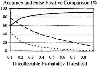
Figure 2 a) shows t11e changes in accuracy of correctly classified calls (good & bad), a standard metric for goodness of tit, correctly classitied bad calls, and falsely classitied good calls over the uncollectible probability t11reshold (from 10% to 90%). The higher t11e uncollectible probability t11reshold, i.e. t11e more conservative we are about classitication, t11e fewer good calls are falsely classified as bad, at t11e expense of t11e fewer bad calls being correctly classitied.

-r-'�----�--s

·

·

·

·

·

·

·

·

·

0 .1

Uncollectible Probability Threshold

--- Correctly Classified Good & Bad Calls

- - - Correctly Classified Bad Calls

• • • - • Falsely Classified Good Calls

Figure 2: Accuracy & Call Volume vs. t11e Uncollectible Probability ll1reshold

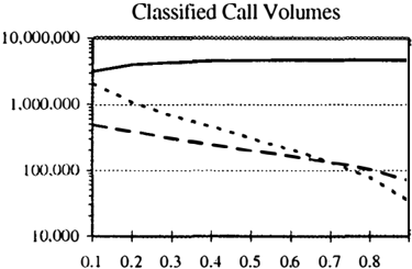
If one were to locus only on accuracy in percentage, one would be quite happy with a lower, more aggressive predicted probability t11reshold since throughout the graph, t11e percentage of correctly classified good calls is larger than t11e percentage of falsely classified good calls. However, because of t11e disparity in volume of classes, simply looking at t11e classitication percentages is not useful; we need to look at call volumes as tl1e predicted probability threshold increases. ·n1e results are presented in Figure 2 b) where t11e Y -axis is in log scale. ll1ere we see that a more conservative approach is indeed warranted. Only at a threshold of around 0.7 do the

correct positives outnumber U1e false positives in tenus of volmne.

5 AUTOMATED ACCOUNT TREAT­ MENT RECOMMENDATIONS USING NORMATIVE EXPERT SYSTEM DEVELOPMENT TOOL

In section 4, we discussed the detection methods and found U1at even using U1e best method, t11e odds of classifying a good customer as uncollectible is still on the order of nJmost 1: 1. Since good customers in U1is segment used in U1e :malysis are some of the most vnluable customers, we do not wish to take an action which may anger U1em and cause t11em to choose an altenmtive long distance comp�my. We U1erefore need to handle customers very carefully. While detcm1ining the probability of uncollectible for each account is very important, we cannot base our actions on this probability alone. For exrunple, we can imagine taking differelll actions based on a customer's profile. ll1cy will have different characteristics based on customer segment, and we want to treat U1em accordingly. If we do tl1is properly with varying degrees of response, we can reduce the number of good customers' complaints as well as reducing the probability of losing them as customers. We can even increase U1e level of customer satisfaction by taking t11e right action.

In U1e telecommunication industry, where there arc a lew hundred million cnlls (several million bad calls) a day, to perfonn this task of detection and ··rational" treatment in real-time witl1 all these uncertainties is not humanly possible wit110ut assistance of a nonnative decision support system such as NESDT.

In descriptive research in psychology, it has been shown Ulat people "systematically violate U1e principle of rational decision making when judging probabilities, making predictions or attempting to cope witJ1 probabilistic tasks. Biases in judgments of uncertainty events are often large and diflicull to eliminate. The source of these biases can be traced to various heuristics or mental strategies that people use to process infonnation" [Siovic, 1977]. The nonnative expert/decision support system is a fonnn.l tool that provides a meru1s to overcome U1ese inherent shortcomings and impose rationality when we face decision making under uncertainty [Hcckemum 1990, Henrion 1992, Ezawa 1993].

We couple t11e APRI Bayesi<m network-based uncollectible model witll NESDT for automated account treaunent recommendation which is based on the influence diagram paradigm. An influence diagram is a generalized Bayesian network wiUl decision and value ; lodes in addition to probabilistic nodes. By evnluating U1is diagrrun, the system recommends the optimnl action given all available infonnation and uncertainties. P reliminary testing of NESDT for automated account treaunent recommendation is currently underway, and we plrul to discuss the results in the coming conference.

6 SUMMARY

We have demonstrated U1e perfornmnce of Bayesian network based supervised machine learning system called APRI in U1e context of a rare binary outcome wiU1 mixed data types and compared it to more classical approaches such as discriminant analysis and CART. APRI's nonparametric approach lends itself well to this class of problems at t11e expense of being very data hungry. However, despite t11e fact that the outcome of interest occurs relatively rarely, t11e telecommunications sector is not exactly a data poor environment. In the comparison to otJ1er metl10ds discriminant analysis proved to be Ule most robust to out-of-sample prediction, i.e. it suffered least from overtitting, while CART was Ule least robust. APRI cmne out al1ead in overall perfonnance and suffered only a little from overfitting tile model to Ule training set.

When we set out to develop a model which would identify potentially fraudulent or uncollectible calls/customers, we were still ignorant of U1e important issue of falsely classifying good customers. In fact, in showing Uwt traditional metl10ds of tluesholding or simple rule based metllOdS and discriminant analysis are not good enough, and t11at U1e "Do Noiliing" alternative outperfom1s t11em, we nlso demonstrated Ulat merely beating t11is "Do NoU1ing" alternative, as U1e Bayesian network model does, is not sufficient. 1l1e handling of predicted uncollectible calls/customers in real-time under uncertainty is not feasible wiUlout intelligent system support, and so U1erefore we introduced a nonnative expert system based on NESDT to handle/recommend appropriate actions based on individual customer information under uncertainty. We believe Ulat U1e combination and active interconnection of a Bayesi!Ul network model based on APRI for identification and intelligent system support based on NESDT for account treaunent recommendation is a constructive and feasible tool for reducing exposure to net bad debt.

Acknowledgements

We wish to t11ank William Cohen, Steve Norton and two anonymous referees for helpful comments and suggestions.

References

• Breiman, L., Friedman, J.H., Olshen, R.A., Stone, C.J., 1984, Classification and Regressing Trees, Wadsworth.
• Catlett, J., 1995, "Tailoring Rulesets to Misclassification Costs", in Preliminary Papers of the Fifth International Worlzshop on Artificial Intelligence and Statistics, 88-94
• Cheeseman, P., Kelly, J., Self, M., Stutz, J., Taylor, W., and Freeman, D., 1988, "AUTOCLASS: A Bayesiru1 Classification System," Proceedings of the Fifth International Conf erence on Machine Learning pp. 54-64, Morgan Kaufmann.
• Cooper G. F., Herskovits E., 1992, "A Bayesi<Ul Method for the Induction of Probabilistic Networks from Data", Machine Learning, 9, 309-347.
• Ezawa, K.J., 1993, "A Nom1ative Decision Support System", Tllird International Conference on Artificial Intelligence in Economics and Management
• Ezawa, K.J., 1994, "Value of Evidence on Influence Diagrams", Proceedings of the Tenth Conference on Uncertainty in Artificial Intelligence, 212-220, Morgan Kaufmann.
• Ezawa, K.J. and Schuermann, T., 1995, ''A Bayesian Network Based Learning System: Architecture and Performance Comparison with Other Methods", to be presented at ECSQARU '95.
• Fukunaga, K., 1990, Introduction to Statistical Pal/ern Recognition, Academic Press.
• Geiger, D., "An Entropy-Based Learning Algorithm of Bayesian conditional Trees", Proceedings of the Eighth Conf erence on Uncertainty in Artificial Intelligence , pp 92-97, Morgan Kaufmann, 1992.
• Heckerman, D.E., 1990, "Probabilistic Similarity Network," Networks, 20, 607-636.
• Heckerman, D.E., Geiger, D., Chickering D.M., 1994, "Learning Bayesian Networks: The Combination of Knowledge ru1d Statistical Data," Proceedings of the Tenth Conference on Uncertainty in Artificial Intelligence, Morgan Kaufmann, pp 293- 301.
• Henrion, M., Breese, J.S., Horvitz, E.J., 1991, "Decision Analysis and Expert Systems," AI Magazine, pp64-91.
• Herskovits, E. H., Cooper, G. F., 1990, "Kutato: An entropy-driven system for t11e construction of probabilistic expert systems from databases", Proceedings of the Conf erence on Uncertainty in Artificial Intelligence, pp 54 - 62.
• Jensen, V., Olesen K. G., and Anderson S. K., 1990, "An Algebra of Bayesian Universes for Knowledge-Based Systems," Networks, 20, 637659.
• Knoke, J., 1982, "Discriminant Analysis with Discrete and Continuous Variables", Biometrics 38, 191200
• Krzanowski, W .J ., 1983, "Distance Between Populations Using Mixed Continuous and Categorical Variables", Biometrika 10, 235-43
• Krzanowski, W.J., 1980, "Mixture of Continuous and Categorical Variables in Discriminant Analysis", Biometrics 36, 493-499
• Langley, Pat and Stephanie Sage, 1994, "Induction of Selective Bayesian Classifiers," Proceedings of the Tenth Conf erence on Uncertainty in Artificial Intelligence, pp399-406, Morgan Kaufman.
• Lauritzen, S. L., and Spiegelhalter, D. J., 1988, "Local Computations with Probabilities on Graphical Structures and their Application to Expert Systems," J. R. Statistics Society, B, 50, No.2 157-224.
• McLachlru1, Geoffrey J., Discriminant Analysis and Statistical Pattern Recognition, John Wiley & Sons, 1992
• Pazzani, M., C. Merz, P. Murphy, K. Ali, T. Hume and C. Brunk, 1994, ''Reducing Misclassification Costs", in Proceedings of the International Conference on Machine Learning, 217-225, Morgan Kaufman
• Pearl, J., 1988, Probabilistic Reasoning in Intelligent Systems, Morgan Kaufmann.
• Provan G. M., Singh M., 1995, "Learning Bayesian Networks Using Feature Selection," Proceedings of International Workshop on AI and Statistics, pp 450 - 456.
• Quinlan, J. R., C4.5 Programs f or Machine Learning, Morgan Kaufmann, 1993.
• Rao, C.R., 1963, "Criteria of Estimation in Large Srunples", Sankhya, Series A., pp.189-206
• Shachter, R. D., "Evidence Absorption and Propagation through Evidence Reversals", Uncertainty in Artificial Intelligence, Vol. 5, pp. 173-190, North-Holland, 1990.
• Slovic, P., Fischhoff, B., and Lichtenstein, S., 1977, "Behavioral Decision Theory," Annu. Rev. Psycho!. 28, 1-39.