Graphical readings of possibilistic logic bases

Salem Benferhat, Didier Dubois, Souhila Kaci and Henri Prade

lnstitut de Recherche en lnformatique de Toulouse (I.R.I.T.)-C.N.R.S. Universite Paul Sabatier, 118 route de Narbonne 31062 TouLOUSE Cedex 4, FRANCE E-mail:{benferhat, dubois, kaci, prade }@irit.fr

Abstract

Possibility theory offers either a qualitative, or a numerical framework for representing uncertainty, in terms of dual measures of pos­ sibility and necessity. This leads to the ex­ istence of two kinds of possibilistic causal graphs where the conditioning is either based on the minimum, or on the product opera­ tor. Benferhat et al. [3] have investigated the connections between min-based graphs and possibilistic logic bases ( made of classi­ cal formulas weighted in terms of certainty ) . This paper deals with a more difficult issue: the product-based graphical representation of possibilistic bases, which provides an easy structural reading of possibilistic bases.

1 Introduction

Possibilistic logic offers a general framework for rep­ resenting prioritized information by means of classical logical formulas which are associated with weights be­ longing to a linearly ordered scale ( and which are han­ dled according to the laws of possibility theory [21]). This leads to a stratification of the information base into layers of formulas according to the strength of the associated weights. This framework can be useful for representing knowledge, and then a weight represents the certainty level with which the associated formula is held for true. A possibilistic logic base can also repre­ sent desires or goals having different levels of priority.

A set of weighted logical formulas, constituting a pos­ sibilistic logic base is semantically equivalent to a possibility distribution which rank-orders the possible worlds according to their levels of possibility. These possibility levels are to be understood as plausibility or normality levels in case the base gathers pieces of knowledge, or as levels of satisfaction of reaching a considered world in case it is a collection of weighted goals.

Apart from the syntactic representation provided by a possibilistic base, an other compact representation, sharing the same semantics is of interest, namely, pos­ sibilistic directed acyclic graphs ( DAGs ) [12, 3]. The merit of the DAG representation is, as usual, to exhibit some independence structure ( here in the possibilistic framework), and to provide a structured decomposi­ tion of the possibility distribution underlying the base. However, the interest of working with different repre­ sentation modes has been pointed out in several works [4, 16].

Depending if we are using a numerical scale such as [0,1], or a simple linearly ordered scale, two types of conditioning can be defined in possibility theory; one based on the product which requires a numerical scale, and one based on minimum operation for which any linearly ordered scale fits. This corresponds to quan­ titative and qualitative possibility theory respectively [9]. In quantitative possibility theory, possibility de­ grees can be viewed as upper bounds of probabilities [8]. Until recently, quantitative possibility theory did not have any operational semantics strictly speaking, despite an early proposal by Giles [13] in the setting of upper and lower probabilities, recently taken over by Walley, De Cooman and Aeyels [20, 5]. One way to avoid the measurement problem is to develop a qual­ itative epistemic possibility theory where only order­ ing relations are used [9]. For quantitative ( subjec­ tive ) possibilities, an operational semantics has been recently proposed [18], [10] which differs from the up­ per and lower probabilistic setting proposed by Giles and followers. It is based on the semantics of the trans­ ferable belief model [17], itself based on betting odds. It can be shown that the least informative among the belief structures that are compatible with prescribed betting rates is a possibility measure. Then, it can be also proved that the min-based idempotent con­ junctive combination of two possibility measures cor-

二

responds to the hyper-cautious conjunctive combina­ tion of the belief functions induced by the possibility measures.

The translation of a possibilistic graph (product­ based, or minimum-based) into a possibilistic logic base has been already provided [2], as well as the con­ verse transformation for minimum-based possibilistic graphs [3]. The translation of a possibilistic logic base into a product-based graph, which is less straightfor­ ward is now addressed in this paper. The transforma­ tion is illustrated on a running example dealing with the goals of an agent.

The paper is organized as follows. After a minimal background on possibility theory, possibilistic logic and possibilistic graphs, the transformation of a pos­ sibilistic logic base into a product-based possibilistic graph is discussed in details in the rest of the paper.

2 Background

2.1 Possibility theory

Let £ be a finite propositionnal language. 0 is the set of all classical interpretations. Greeck letters ¢>, '1/; · · · denote formulas. The notation w f= ¢> means that w is a model of ¢>.

A possibility distribution [21]7r is a function mapping a set of interpretations (or worlds) n into a linearly ordered scale, usually the interval [0, 1]. 1r(w) rep­ resents the degree of compatibility of the interpreta­ t i o n w w i t h the available beliefs about the real world in a case of uncertain information, or the satisfaction degree of reaching a state w, when modelling prefer­ ences. rr(w) = 1 means that it is totally possible for w to be the real world (or that w is fully satisfactory), 1 > rr(w) > 0 means that w is only somewhat pos­ sible (or satisfactory), while 1r(w) = 0 means that w is certainly not the real world (or not satisfactory at all). A possibility distribution is said to be normalized (or consistent) if 3w s.t. 1r(w) == 1. Only normalized distributions are considered here.

Given a possibility distribution 1r, two dual measures are defined which rank order the formulas of the lan­ guage:

1. The possibility (or consistency) measure of a for­ mula¢>:

which evaluates the extent to which ¢is consistent with the available beliefs expressed by 1r.

1. The necessity (or certainty) measure of a formula ¢:

which evaluates the extent to which ¢> is entailed by the available beliefs.

When dealing with knowledge, a statement ¢ is thus estimated in terms of two measures II and N w h ic h enable us to differenciate between the certainty of -.cf> ( N ( -.¢) ::;;: 1) and the total lack of certainty in ¢> (N(¢) = 0). When dealing with desires N(cf>) refers to the imperativeness of goals ¢>, while II(¢) estimates how satisfactory is to reach ¢>.

The definition of conditioning in possibility theory de­ pends if we use an ordinal, or a numerical scale. In an ordinal setting, min-based conditioning is used and is defined as follows:

In a numerical setting, the product-based conditioning is used:

Moreover, ifiT(cf>) = 0, then II('�/; I¢)= IT(-..,p I¢)= 1.

Both forms of conditioning satisfy an equation of the form: II ( � ) ::;;: D(IT(� I ¢>), II( ¢> )), which is similar to Bayesian conditioning, for 0 = min or product. In this paper we privilege the numerical setting.

It is clear that ;r'(w) = 1r(w I ¢), the result of con­ ditioning a possibility distribution 1r with ¢ is always normalized.

2.2 Possibilistic knowledge bases

A possibilistic knowledge base is a set of weighted for­ mulas of the form�= {(¢;,a:;) : i = 1, n} where cp; is a classical formula and, a:; belongs to [0, 1] in a nu­ merical setting and represents the level of certainty or priority attached to cf>;.

Given a possibilistic base I:, we can generate a unique possibility distribution rr�, where interpretations will be ranked w.r.t. the highest formula that they falsify, namely [6]:

Definition 1 'Vw E 0,

Example 1 Let su, wi, se be three symbols which stand for "sun", "wind" and ''sea" respectively. Let I: be the following possibilistic base:

These rules express the goals of somebody who likes basking in the sun, or going windsurfing (which re­ quires wind and sea). The most prioritized formula expresses that the person strongly dislikes to have wind in a non-suny day, while the other less prioritary goals express that she dislikes situations with wind but with­ out sea, or with sea without wind, or with neither sun nor sea.

Let n = {wo = su /\ ·wi /\ ·se, wl = su /\ ·Wi /\ s e , w2 = su /\ wi /\ ·se, ws = su /\ wi /\ se, w4 = -,su /\ ·wi /\ -,se, w5 = ·su 1\ -,wi /\ se, w6 = -, s u /\ wi 1\ ·se, W7 = ·su 1\ wi 1\ se}.

Let 7rE be the possibility distribution associated with :E: 7rE(wo) = 7rE(ws) = 1, 1rE(w1) = 7rE(w2) = 7rE(w4) = 7rE(ws) = � and 7rE(w6) = 7rE ( W 7 ) = �·

The converse transformation from 1r to :E is straight­ forward. Let 1 > /31 > · · · > f3n :;::: 0 be the differ­ ent weights used in 1r. Let r/J; be a classical formula wl;wse models are those having the weight /3; in 1r. Let E = { ( -.rp;, 1 - /3;) : i = 1, n}. Then, 7rE = 1r.

We now give further definitions which will be used lat­ ter in the paper:

Definition 2 Let :E be a possibilistic knowledge base, and a E [0, 1). We call the a-cut (resp. strict a-cut) of:E, denoted by :E>a (resp. :E>a), the set of classical formulas in :E havi ; g a certainty degree at least equal to a ( resp. strictly greater than a).

Inc(:E) =max{ a; : :E�a, is inconsistent} denotes the inconsistency degree of :E. When :E is consistent, we have I n c( :E ) = 0.

Subsumption can now be defined:

Definition 3 Let (rp, a) be a formula in E. Then, (rp,o:) is said to be subsumed in:E if (:E-{ (rp,a)}h<> f­ rp. (rp, a) is said to be strictly subsumed in :E if E>a fr/J.

Indeed, we have the following proposition [6]:

Proposition 1 Let :E be a possibilistic knowledge base, and (rp, a) be a subsumed formula in :E. Let :E' = :E- {(¢;, o:)}. Then, :E and :E' are equivalent I. e. 7rE = 7r E '.

2.3 Possibilistic networks

Another possibilistic representation framework of un­ certain information is graphical and is based on con­ ditioning. Information is then represented by possi­ bilistic DAGs (Directed Acyclic Graphs) [3, 12], where nodes represent variables (in this paper, we assume that they are binary), and edges express influence links between variables. When there exists a link from A to B, A is said to be a parent of B. The set of parents of a given node A is denoted by P a r( A). By the capital letter A we denote a variable which represents either the symbol a or its negation. An interpretation in this section will be simply denoted by A 1 · · · An, or by w.

Uncertainty is expressed at each node in the follow­ ing way:

-For root nodes A; (namely Par(Ai) = 0) we pro­ vide the prior possibility of a; and of its negation -.a;. These priors should satisfy the normalization condi­ tion:

- For other nodes Aj, we provide conditional possibility of aj and of its negation -.ai given any complete in­ stantiation of each variable of parents of Aj, w Par(A i ). These conditional possibilities should also satisfy the normalization condition:

A product-based possibilistic graph, denoted by lTG, induces a unique joint distribution using a so-called chain rule:

Definition 4 Let lTG be a product-based possibilistic graph. The joint possibility distribution associated with II G is computed with the following equation (called chain rule):

rr(w) =*{II( a I WPar(A)) : w f= a and w f= WPar(A)}, where * = product.

The converse transformation from a possibility distri­ bution 1r to a product-based graph is straightforward. Indeed, given an interpretation w = A1A2 ···An, we have:

Applying repeatedly the Bayesian-like rule for an arbi­ trarily ordering A1, ···,An between variables, we get: 1r(A1 ···An)= 1r(A1 I A2 ···An)* 1r(A2 I A3 ···An)*···* 7r(An-1 I An)* 7r(An)·

This decomposition is possible since the product is as­ sociative. The decomposition leads to a causal possi­ bilistic graph where parent of A; are {Ai+l, ···,An}· It is clear that for the same joint distribution, we can construct several causal possibilistic graphs depending on the choice of the ordering between variables.

In possibility theory, there are several definitions of in­ dependence relations (see e.g. [11),[1]). In this paper, since we deal with product-based conditioning, we will use the following definition of independence, namely: rp and 1./J are independent if II( 1./J I rp) = II( 1./J).

一

3 From possibilistic bases to product-based graphs : Basic ideas

In [2], the authors have provided the transformation of possibilistic graphs to possibilistic bases. In [3], the transformation from 1: to a min-based graph, where conditioning is based on minimum operation rather than on the product, has been given.

In the following, we provide the transformation from a possibilistic base 1: to a product-based graph IIG. This transformation is different from the transformation in case of conditioning based on the minimum operation. However there is one common step in both approaches which consists in putting the knowledge base into a clausal form and in removing tautologies.

The following proposition shows how to put the base in a clausal form:

Proposition 2 {6} Let 1: be a possibilistic base. Let (¢,a) be a formula in 1:, and { ¢ 1, · · · ,¢ n } be the set of clauses encoding ¢. We define E' obtained by replac­ ing each formula(¢, cr ) in E by {(¢1, a ) ,···, (¢n, a)}. Then, 1: and E' are equivalent i.e., 7rE = 7rE'.

The removing of tautologies is important since it avoids fictitious dependence relations between vari­ ables. For example, the tautological formula ( ---, x V ---,y V x, 1) might induce a link between X andY.

The basic idea in the transformation from the knowl­ edge base to a possibilistic graph is first to fix an ar­ bitrarily ordering of variables A1, · · · , An. This order­ ing means that the parents of A; should be among A;+l, · · ·,An (however it can be empty). Then we proceed by successive decompositions of 1:, which is associated with the above decomposition of a possibil­ ·ity distribution rr, namely:

The result of each step i is a knowledge base associated with rr ( A; ···An ) . Moreover, this resulting base will enable us to determine Par(A;) the set of parents of A; and to compute the conditional possibilities rr(A; I P a r ( A ; ) ) .

In the following, we will only consider the first step (i = 1), and we will denote by Ec (C for Current) the base associated with rr(A2 ···An ) · The procedure of this first step can be then iterated at each step. Ec is called the marginalized base.

The computation of Ec is provided in the next section, then in Section 5 we show how to determine parents of each node, and lastly in Section 6 we compute the conditional possibility degrees.

4 Computation of the marginalized base �c

The computation of Ec involves three tasks:

• decomposing a possibility distributions rr into its restriction on a1 and its negation ---,a1 (recall that at and ...,at are the two only instances of At),
• marginalisation of these two distributions for get­ ting rid of At,
• the effective computation of Ec.

4.1 Decomposing rr

Let us first define two possibility distributions rra1 and rr -,a1 in the following way:

7ra1 (resp. rr.,aJ are very similar to conditioning ex­ cept that we do not normalize after learning at (resp. -,at). 11'a1 and rr...,a1 are simply the decomposition of rr. Indeed, it can be checked that:

Example 2 We consider again the possibilistic base E of Example 1. Let us compute rr·e and 1!'...,.6· We get:

Then, we can check that

'Vw, 1T'E(w) = max(7r38(w), 7!'.,.6(w)) where 7r E is the possibility distribution associated with E.

We can easily check that the possibilitic bases associ­ ated with these distributions are given by:

Proposition 3 The possibilistic base associated with rra, (resp. rr ..... a,) is l: U { ( a t , 1)} ( resp. EU{(---,a1, 1)}}.

Proof

The proof is obvious. Indeed, we have two cases:

• w p!: a1, then using Definition 1: 7l'Eu{(a1, 1 )}(w) = 1 max { a; : ( ¢;, a; ) E 1: U {( at , 1)}, w p!: <Pi } = 0 (since w p!: al)

The two following lemmas give two simplifications of I: U {(at, 1)} ( resp. L U {(-.a1, 1) } ) .

Lemma 1 Let I:� = E U {(a1, 1)}. Let I:J.' = E!­ {(at V x, a) : (a V x,a) E E} a base obtained from E! by removing clauses containing at. Then, I:! and EJ.' are equivalent, in the sense that they generate the same possibility distribution which is 1r a1·

The proof is obvious since (at V x, a) is subsumed by (a1, 1).

Lemma 2 Let E! = EU{(at, 1) }. Let LJ.' be the possi­ bilistic base obtained from E! by replacing each clause of the form ( · a t V x, a::) by (x, a:: ) . Then, E! and I:J.' are equivalent.

The proof can be again easily checked. Indeed, (a1, 1) and ('at V x, a::) implies (x, a::) which can be added to Lt. And once (x,o:) is added, ( · a t V x, o:) can be retrieved since it is subsumed by (x, a::).

4.2 Marginalisation

In this section, we are interested in computing the marginal distributions from 7ra1 ( resp. 11"-.a tl defined on {A2, .. ·,An}·

Let us denote La, ( resp. L-.a,) the result of the ap­ plication of Lemmas 1 and 2 to I: U {(at, 1)} ( resp. E U { ( ·at, 1) } ), namely the result of removing clauses of the form ( x V at, a) from I: and the result of replac­ ing (x V ' a t , a:: ) by (x, a). Therefore, the only clause in I: a 1 which contains a1 is (at, 1).

Let us denote 1r:,', 1r��� the result of marginalisation of 7r a 1 and 11"-.a, on {A2, ···,An}, namely:

Example 3 Let At = SE. Then,

Also,

NB. ITa, (A2 · · ·An) is the possibility measure associ­ ated with 7ra1 defined on {At,·· ·,An} ·

The following lemma provides the syntactic counterpart of 1r A1 ( resp 1r A ' ) · a1 · ·a1 ·

Lemma 3 The possibilistic base associated with 1r A 1 A . a, (resp. 1r,�) ts Ea, -{(at, 1) } (resp. E-.a1 - {( ' a t, 1)}).

Proof

The proof is obvious. First, note that the only clause containing at in Ea, is (a1, 1). Then,

4.3 Effective computation of I:c

Given Lemma 3 we are now able to provide the possi­ bilistic base associated with 1r(A2 · · ·An) by noticing that:

Example 4 We again consider the possibility distri­ butions 1r!eE and rr�fe computed in Example 3. We have:

1r(su A -,wi) = rr(su A wi) = 1, 1r(...,su A -,wi) = � and 1r(..,su 1\ wi) = � ·

Proposition 4 Let Et = Ea, - {(at, 1)} and I:2 = L-.a, {(·a t , 1) }. The possibilistic base associated with 1r(A2, · ··,An) is:

Proof

The proof is obvious, indeed: 1t"r;c(w) 1 max{min(a;,/3j) : (¢>;, a;) E .Et,('I/Jj,/3j) E L2, w � ¢1; V 'I/Jj} = 1-min{max{a;: (¢;,a::;) E Et,W � ¢;}, max{f3J: ('I/J j , /3j) E E2,w � '1/Jj}} =max{!- max{ a::; : (¢;, a::;) E .Et, w � ¢;}, max{fJJ ('I/Jj,/3j) E 2, w '1/J J}} 0

4.4 Summary

Let us now summarize the computation of Ec:

1. Add (a1, 1) ( resp. ('at, 1)) to E,
2. Remove clauses containing a t ( resp. -,at ) of the form (a1 V x, a) ( resp. ('at V x, a)),

一

1. Replace clauses of the form ( ' a t V x, a) ( resp. (at V x, a)) by (x, a).

Let E1 (resp. E2) the result of the Step 3. Then, Ec = {(¢> V 1/J, min(a, ,8)) : (¢>, o:) E Et- {(at, 1)}, (.,P,,B) E E2-{( ' a t , 1)}}.

Example 5 Let us consider our example again. Let {SE, WI, SU } be the ordering of the variables (namely At = SE, A2 = WI, and A3 = SU ) . We start with the variable SE.

Let us compute Ec the possibilistic base associated with 1rB(A2A3) (namely, 11'E(W I A SU)).

We first add "se" with a degree 1, we get:

{(wi V -,se,k),(-,wi V se,k),(su V se,�),(su V -,wi, �), ( se, 1)}. Then we remove clauses containing se (except the added one), we get {(wi V -,se, k), ( s u V --, w i , �), (se, 1)}. Then we replace all clauses of the form ( ¢> V ·se, a) by ( ¢> , o: ) we get: E,e = {( wi, k ) , (su V -,wi, j), (se, 1)}. Similarly, for -,se: E...,u = {(-,wi, k), (su, k), (su V -,wi, �), (-, s e,1)}. Finally, using Proposition 3 we have: Et = { ( w i , �), (su V -,wi, �)}, E 2 = {(-,wi, �), ( s u, �), (su V -,wi, � )} and Ec = {(su, �), (su V --,wi, �)}. 11'(WI 1\SU), the possibility distribution computed in Ex­

It can be checked that 11'E0(WI 1\SU) = where 11' is ample 4.

The problem of finding a syntactic counterpart of the marginalization process is clearly similar to the marginalization problem addressed in [15]. Their ap­ proach is more based on successive resolution in order to compute the marginalization base. Another small difference is that their approach is proposed in the clas­ sical case, without levels of priorities. Both procedures are polynomial.

5 Determining parents of A1

We are interested in determining P a r(A1) which are the parents of At. This set should be such that:

TI(At

I

A

2

·

·

·

A

n

)

=

TI(At

I

Par(Al)).

Once parents of At are determined, we compute the conditional possibility degrees TI(At I Par(At)) in Sec­ tion 6.

The determination of parents of At is done in an incre­ mental way. First, we take Par(At) as the set of vari­ ables which are directly involved at least in one clause containing at or --,a1. Par(A1) are obvious parents of At. However, it may exist other "hidden" variables, whose observation influences the conditional possibil­ ity TI(A1 I Par(At)). To show this, let us give the following illustration:

Example 6 Let E = {(a2 V a t , .4), (a3, .7)}, then we can easily check in context -,a2, at is deduced to a degree .4, which means that TI( -,at I -,a2) = 1-.4 = .6. However, in context ....,a2...,a3 the certainty of a1 is now o, which means that n(...,ar 1 -.a2-.a3) = 1 - o = l(due to presence of a conflict in E U { 'a2 1\ ...,a3}). Hence A3 should also be considered as a parent of At, even if it is not directly involved. (see {6] for the presentation of the inference machinery in possibilistic logic). Algorithm 1 provides the computation of Par(A1). Algorithm 1: Determining_Parents_oLAt Data: E Result: Parents of At begin 1. Finding immediate parents of At l.a. LA1 +-{(¢>;,a;):(¢>;, a;) E E and ¢>; contains either at or -, at }. l.b. Par(At) +-{V: 3(¢;, o:;) E E A1 containing an instance of V} 2. Checking for hidden parents 2.a. B +-E, let (xt, · · · , Xn) be an instance of Par( At) 2.b. Remove from Beach clause containing x;, 2.c. Replace in B e ach clause of the form (....,x, V --,Xj"' V ....,xk V ,P,o:) by (,P,o:) 2.d. Let o: ( resp. ,8) be the certainty degree of at ( resp. -,at) from BU{(xt, 1), · · · , (xn, 1)} 2 . e . if there exists ( ¢>, 7) E B such that 7 2: o: (resp. 7 2: ;3), then: Par(Al) = P a r ( At) U { V : ¢> contains an instance of V} Go to Step 2 return Par(At) end

Let us briefly explain this algorithm. The first step simply starts with parents of At, the set of variables which are directly linked with At. Step 2 checks for hidden parents of At, namely if P a r ( At) can be ex­ tended or not.

A set of variables V has to be added to Par(At), if there exists an instance (x1, · · · , xn) for Par(At) such that:

II(at I X t X 2 · · ·Xn) fTI(at I XtX2 · · ·Xnv). (resp. TI(-.at I XtX2 · · ·Xn) =j:. II(--,at I XtX2 · · ·xnv)), where v is an instance of V. The computation of II( 'at I Xt · · · Xn ) can be done syntactically from E U {(xt, 1), · · ·, (xn, 1)} (for a formal computation of IJ ( -, a t I Xt· · ·Xn) see Section 6).

This is what it is done in Step 2, by checking if any additional variables can have influences on II(at I Xt · · ·xn) · To achieve this goal, we first as­ sume that (x1, 1), · · · , (xn, 1) are true. Step 2.b re­ moves (x; V </;,a) since the latter are subsumed. Step 2.c replaces (-.x; V · · · V -.xk V </;,a) by (</;,a) since (-.x; V ···V-.xk V</;,a) and {(x;,1),···,(xk,1)} im­ plies (</;,a) which subsumes ( -.x; V · · · V -.xk V </;,a) .

Now, assume that B U {(xi, 1), · · ·, (xn, 1)} 1(at, a) (Step 2.d and 2.e). Let (</;,J) E B, such that J > a. Then, variables which are in ¢1 should be added to Par(Al). Indeed, let ¢1 = v1 V · · ·Vvn. Then, one can easily check that:

II( at I Xt · · ·Xn-,V! · · ·-.vn) # IT(a1 I Xt · · ·Xn), because B U { ( x i , 1), . . · , ( -.vi, 1), · · · , (-.vn, 1)} is i n­ consistent to a degree 2: J from which a1 can no longer be inferred.

{ ( su V

Example 7 Let us consider again the base L: = -.w i , �), ( -.wi V se, �), (wi V -.se, �), (su V se, �)}. Then, using the above algorithm we get: Par(SE) = { WI , SU}, Par(W I) = {SU} and Par(SU) = 0.

6 Computation of conditional possibility degrees

This subsection shows how to compute II(A1 Par(Al)) once Par(At) is fixed. Let (x1,· · ·,xn) be an instance of Par(At), and a1 an instance of A1· Recall that by definition:

The following proposition provides the computation of II ( ql) syntactically:

Proposition 5 II(</;)= 1- Inc(L: U {(ql, 1)}). (We recall that L: is assumed to be consistent).

The proof is immediate since II( ql) = 1 -N ( -.q,), and that N(-.ql) = Inc(L: U {(¢, 1)}) (See [ 6 ]). Therefore, to compute II(at I Xt· · ·Xn):

1. Add {(x1, 1), · · · , (xn, 1)} to :E. Let L:' be the re­ sult of this step.
2. C o m put e h II(x1 · · · Xn )) 1 -I nc(L:') ( h represents
3. Add {(a1, 1)} to L:'. Let L:" be the result of this step.
4. -represents
5. Compute h1 1 I nc(L:") (h' II(atXt · · ·Xn)) . Then, { 1 ifh=O II ( al I X t .. . Xn) = If otherwise.

Example 7 (continued)

Let us illustrate the computation of IT( -.se I wi 1\ su). We get L:' = {(wi, 1), (su, 1), (suV-.wi,i), (-.wi V se, �), (wi V -,se, �)}.

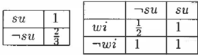
Hence, II( -.se 1\ wi 1\ su ) = �. Lastly: II( -,se wi 1\ su) = !f = l following conditional possibilities:

We add the instance {(wi,l),(su,l)} toE (Step 1). (suVse, �), We have I n c ( L: ') = 0. Then, h = 1 {Step 2). We now add (-.se, 1) to L:' (Step 3). We get L:" {(-.se, 1 ), (wi, 1), (su, 1), (su V -.wi, i), (su V se, �), (-.wi V se, �), (wi V -.se, �)}. We have Inc(L:11) = �-Then, h' = �· With a similar way, we get the =

w� -.wz

---.su � 1

s u 1 1

II(SE I WI, SU)

	-. w z s u	-.wz-.su	WZSU	wi ---. s u
se	�	1	1	1
-.s e	1	1		1

..

�

It can be checked that the possibility distribution asso­ ciated with the constructed 11 G (using the chain rule) is the same as the one associated with the possibilistic base.

Observe that we have chosen the ordering of the vari­ ables in the example arbitrarily. Clearly each appli­ cation suggests orderings which are the more natural ones, or which leads to a simple structure. Note also that the computation of the weights could be also han­ dled symbolically.

7 Conclusion

In the possibility theory framework, desires or knowl­ edge can be equivalenty expressed in different formats. This paper has used two compact representations of possibility distribution: a possibilistic knowledge base and possibilistic graph.

Each of these representations have been shown in pre­ vious papers [3, 6] to be equivalent to a possibility distribution which rank-orders the possible worlds ac­ cording to their level of plausibility. The framework may use a symbolic discrete linearly ordered scale, or can as well be interfaced with numerical settings by us­ ing the unit interval as a scale, using a different type of conditioning in each case [9].

This paper is on step further in establishing the rela­ tionship between different compact representation of possibility distribution. The results presented in this paper would enable us also to translate a possibilistic logic base easily into a kappa function graph [14] since

二

there exists direct transformations [7] b e t w e en possi­ bility theory and Spohn's ordinal conditional functions [19].

References

• [lJ N. Ben Amor, S. Benferhat, D. Dubois, H. Geffner, and H. Prade. Independence in qual­ itative uncertainty frameworks. In Seventh Inter­ national Conference on Principles of Knowledge Representation and Reasoning (KR '2000), Breck­ enridge, Colorado, April 11-15, pages 235-246. Morgan Kaufmann, 2000.
• S. Benferhat, D. Dubois, L. Garcia, and H. Prade. Directed possibilistic graphs and possibilistic logic. In 15th International Conference on In­ formation Processing and Management of Uncer­ tainty in Knowledge-based Systems (IPMU'98), Paris, pages 1470-1477, 1998.
• [ 3] S. Benferhat, D. Dubois, L. Garcia, and H. Prade. Possibilistic logic bases and possibilistic graphs. In 15th Conference on Uncertainty in Artificial Intelligence (UAI'99), Stockholm, pages 57-64, 1999.
• C. Boutilier, T. Deans, and S. Hanks. Deci­ sion theoric planning: Structural assumptions and computational leverage. Journal of Artificial Intelligence Research, 11:1-94, 1999.
• G. De Cooman and D. Aeyels. Supremumpreserving upper probabilities. Information Sci­ ences, 118:173-212, 1999.
• D. Dubois, J. Lang, and H. Prade. Possibilistic logic. In Handbook of Logic in Artificial Intelli­ gence and Logic Programming, 3, Oxford Univer­ sity Press:pages 439-513, 1994.
• D. Dubois and H. Prade. Epistemic entrench­ ment and possibilistic logic. Artificial Intelligence, 50:223-239, 1991.
• D. Dubois and H. Prade. When upper proba­ bilities are possibility measures. Fuzzy sets and Systems, 49:65-74, 1992.
• D. Dubois and H. Prade. Possibility theory: qual­ itative and quantitative aspects. In Handbook of Defeasible Reasoning and Uncertainty Man­ agement Systems. (D. Gabbay, Ph. Smets, eds.), Vol. 1: Quantified Representations of Uncer­ tainty and Imprecision, ( P h . Smets, ed.) Kluwer, Dordrecht:169-226, 1998.
• D. Dubois, H. Prade, and P. Smets. New seman­ tics for quantitative possibility theory. In 6th Eu­ ropean Conference on Symbolic and Quantitative
• Approaches to Reasoning and Uncertainty (EC­ SQARU'Ol), Toulouse. Springer, LNAI, to ap­ pear, 2001.
• P. Fonck. Conditional independence in possibility theory. In 10th International Conference on Un­ certainty in Artifcial Intelligence (UA/'94), pages 221-226, 1994.
• J. Gebhardt and R. Kruse. Possinfer - a software tool for possibilistic inference. In Fuzzy set Meth­ ods in Information Engineering. A Guided Tour of Applications (D. Dubois, H. Prade, R. Yager, eds.), Wiley, 1997.
• R Giles. Foundations for a possibility theory. In F uzz y Information and Decision Processes, pages 83-195. (M. M. Gupta and Sanchez, eds.), North Holland, Amsterdam, 1982.
• M. Goldszmidt. Belief-based irrelevance and net­ works: Towards faster algorithms for prediction. In AAAI'94 Fall Symposium Series: Relevance. http:/ jwww.pitt. edu/ druzdzeljpapersjmoises.html, pages 89-94, 1994.
• J. Kohlas, R. Haenni, and S. Moral. Propositional information systems. Journal of Logic and Com­ putation, 9(5):651-681, 1999.
• D. Poole. Logic, knowledge representation, and Bayesian decision theory. In Computational Logic -CL 2000, pages 70-86. LNAI 1861, Springer, 2000.
• P. Smets. The transferable belief model for quan­ tified belief representation. In Handbooks of De­ feasible Reasoning and Uncertainty Management Systems, Vol. 1, pages 267-301. (D. Gabbay and P. Smets, eds.) Kluwer, Dordrecht, 1998.
• P. Smets. Quantified possibility theory seen as an hyper cautious transferable belief model. In Ren­ contres Francophones sur la Logique Floue et ses Applications, pages 343-353. Cepadues, Toulouse, 2000.
• W. Spohn. Ordinal conditional functions: a dy­ namic theory of epistemic states. In Causation in Decision, Belief Change, and Statistics, Vol. 2:pages 105-134, 1988.
• P. Walley. Statistical inferences based on a second-order possibility distribution. Interna­ tional Journal of General Systems, 26:337-383, 1997.
• L. Zadeh. Fuzzy sets as a basis for a theory of possibility. Fuzzy Sets and Systems, 1:3-28, 1978.