HUGS: Combining Exact Inference and Gibbs Sampling in Junction Trees

Uffe Kjrerulff

Department of Mathematics and Computer Science, Aalborg University Fredrik Bajers Vej 7E, DK-9220 Aalborg 0, Denmark [email protected]

Abstract

Dawid, Kjrerulff & Lauritzen (1994) provided a preliminary description of a hybrid between Monte-Carlo sampling methods and exact lo­ cal computations in junction trees. Utiliz­ ing the strengths of both methods, such hy­ brid inference methods has the potential of expanding the class of problems which can be solved under bounded resources as well as solving problems which otherwise resist ex­ act solutions. The paper provides a detailed description of a particular instance of such a hybrid scheme; namely, combination of ex­ act inference and Gibbs sampling in discrete Bayesian networks. We argue that this com­ bination calls for an extension of the usual message passing scheme of ordinary junction trees.

1 INTRODUCTION

This paper presents an extension of the expert system shell Hugin (Andersen, Olesen, Jensen & Jensen 1989), called HUGS ("Hugin +Gibbs sampling"), involving a subset of the functionality described by Dawid et al. (1994). The extension involves the introduction of a new kind of belief universe, called a GIBBS universe. This has a dramatic impact on both the compilation process and the various inference steps performed in a junction tree.

Compiling a Bayesian network involves construction of a junction tree (Jensen 1988) via the processes of mor­ alization and triangulation (Lauritzen & Spiegelhalter 1988). Inference in the Bayesian network is then for­ mulated in terms of message passing in the junction tree (Jensen, Lauritzen & Olesen 1990). A node, U, of a junction tree is called a belief universe (or simply a universe) and consists of

• a cluster of variables of the Bayesian network and
• a set of potential functions (or simply potentials), cpu, defined on these variables.

Provided the independence graph of the Bayesian net­ work is a directed acyclic graph, cpu is initially a set of (conditional) probability functions, where each func­ tion is defined on a variable (the child) and a set of conditioning variables (the parents) such that both the child and its parents are members of U. Later, when messages are being passed to U from its neighbours V, . . . , W, cpu is extended with functions defined on U n V, . . . , U n W, where we use U etc. as shorthand for 'the variables associated with U'. These intersec­ tions are called separators (Jensen et al. 1990) (consult this reference for further details on the definition and properties of junction trees).

Hence, a universe, U, may be considered an au­ tonomous entity containing local knowledge (i.e., cpu). Absorption of messages possibly improves this knowl­ edge, and eventually, when U has received active mes­ sages from each of its neighbours, it has got sufficient information to calculate the true joint (probability) distribution over its variables. (A message is called active if the sender has received active messages from each of its neighbours, with the possible exception of the recipient, and it is the first message from the sender to the recipient with that property (Dawid 1992). FUr­ ther, when an active message has been sent in each direction along each link of the junction tree, equilib­ rium has been established (i.e., each universe contains complete information to calculate the true joint distri­ bution over its variables). The process of establishing equilibrium is also termed propagation and involves an inward and an outward pass with the inward pass be­ ing completed when only one universe is capable of sending an active message (in which case exactly one active message has been passed along each link of the junction tree).)

At any time, the exact joint potential, tfou, of a uni­ verse, U, is calculated as the product of the current potentials in 4>u. H all variables of U are discrete and U calculates tfou, we shall refer to U as a DE uni­ verse, where 'DE' stands for 'discrete exact'. Note that the complexity of calculating tfou may be expressed through the complexity of the complete subgraph in­ duced by U (or, in other words, the independence graph induced by tfou is complete, since tfou itself does not carry explicit information about its original fac­ torization). In many real-world applications, the cal­ culation of tfou is prohibitive due to the size of Xu (the configuration space of U). Then a possible fruitful al­ ternative (as suggested in the present paper) could be to approximate tfou through simulation (i.e., establish­ ing a potential J>u � tfou through repeated sampling of the potentials in 4> u).

If the calculation of the joint potential is approximated through Gibbs sampling (Geman & Geman 1984), we shall refer to U as a GIBBS universe. Note that the complexity of calculating J>u is proportional to the complexity of the moral graph induced by 4>u (i.e., the moral graph of the union of the independence graphs induced by the potentials in 4>u) provided that vari­ ables are only sampled simultaneously when necessary. However, to ensure convergence, it is often necessary to sample 'blocks' of variables simultaneously; thus in HUGS we use an advanced Gibbs sampling device (Jensen, Kong & Kjrerulff 1995). We shall elaborate on the issue of blocking-Gibbs sampling in Section 2.

A message sent via a separator S may be perceived as a list of configurations and associated weights. Con­ figurations with no explicit weight associated are as­ sumed to have weight zero. If the message contains a non-negative weight for each x E Xs, the message is complete; otherwise, it is incomplete. Note that in order to avoid conflicts, two or more incomplete mes­ sages cannot, in general, be absorbed simultaneously. This calls for an extension of the message-scheduling vocabulary and management as discussed in Sections 5 and 6.

The motivation for introducing GIBBS universes is twofold. First, as already discussed, the computational complexity imposed by a GIBBS universe is not ex­ ponential in the number of variables of the universe. Second, the use of Monte-Carlo type ai.gorithms for in­ ference makes it possible to handle a larger range of distributions and mixtures of distributions. In HUGS, however, we have limited the functionality to ordinary discrete-type Bayesian networks.

Thomas, Spiegelhalter & Gilks (1992) have described a general program, called BUGS, for Bayesian inference in graphical structures using Gibbs sampling. How- ever, contrary to HUGS, BUGS relies exclusively on Gibbs sampling, but is able to handle a wide range of continuous as well as discrete distributions.

Section 3 presents a (small) example used throughout the paper to illustrate some relevant issues of propaga­ tion in HUGS. In Sections 4-8 we shall provide detailed descriptions of message format, message generation in a GIBBS universe, and message scheduling. Section 9 briefly discusses possible future extensions of HUGS.

2 GIBBS SAMPLING

When a GIBBS universe, U, has completed sampling (i.e., an approximation J>u of tfou has been found), U becomes a DE universe in the sense that all subse­ quent absorptions and generations of mes�ages will be performed in the usual DE manner using tfou (or modi­ fications of it). To see why U cannot perform sampling in both the inward and the outward pass of propaga­ tion, it might be helpful to express J>u as the product of tfou and a 'disagreement' function 6u which can be considered an evidence (or likelihood) function. That is, in a sense, the error imposed when generating J>u amounts to inserting evidence into U. Then, obvi­ ously, performing sampling in the outward pass would require another propagation, which in turn would re­ quire yet another, etc. So, sticking to a two-pass ap­ proach, GIBBS universes must change status to DE whenever they have performed sampling.

Gibbs sampling is characterized by imposing a neigh­ bouring structure onto the configuration space, say Xu, from which the samples are drawn. That is, the samples are dependent in the sense that, given a par­ ticular current configuration, only a (small) subset of Xu will be candidate next configurations. The topol­ ogy of the neighbouring structure depends heavily on the extent to which variables are sampled simultane­ ously: the greater the number of variables sampled si­ multaneously the denser the neighbouring structure. Further, the denser the neighbouring structure the larger the independence between samples and, conse­ quently, the faster the convergence. So, finding an optimal balance between complexity and rate of con­ vergence is essentiaL

Consider, for example, a universe, U, containing two binary variables XA and XB with XA = {a1,a2} and XB = {b1,b2}· Assume that 4>u = {<pu,1/JB}, where <pu(al,bt) = <pu(a2,b2) = 1, <pu(at,�) = <pu(a2,bi) = 0, and 1/JB(XB) = (z,l- z). Let (a1,b1) be the initial configurati?n. Then samplin� XA and XB individually, we get rfou(a1.b1) = 1 and rfou(y) = 0 for y E Xu\ {(at,b1)}. Sampling XA and XB si­ multaneously, on the other hand, we get the correct answer, namely J>u(a1,bl) -+ z, J>u(a2,b2) -+ 1 z,

and ¢u(al,b2) = ¢u(a2,bl) = 0. In the first case, the neighbouring structure is characterized by a dis­ connected graph, whereas, in the second case, it is a complete graph. The Markov chains induced are also said to be, respectively, reducible and irreducible.

Blocking-Gibbs sampling cannot, in general, guarantee irreducibility except, of course, in the degenerate case where all variables are sampled simultaneously. Vari­ ous stochastic relaxation techniques, like simulated an­ nealing, can be employed to guarantee irreducibility with probability arbitrarily close to 1, but this out of the scope of the present paper.

3 AN EXAMPLE: AUNT EMILY

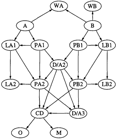
The example chosen to illustrate the features of HUGS is the Aunt Emily network displayed in Figure 1 (a toy example for revealing the cause of death for two elderly, wealthy ladies who have heart troubles and unscrupulous and greedy heirs).

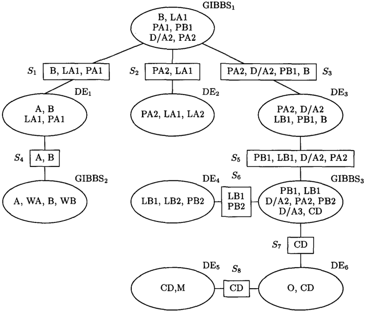
A hybrid junction tree (i.e., a junction tree containing both DE and GIBBS universes) for the Aunt Emily network is displayed in Figure 2.

The distribution of potentials (conditional probabil­ ity functions) over the various universes is handled as usual, except that the potentials are stored in differ­ ent ways in the two kinds of universes and that GIBBS universes are preferred to DE universes for the sake of efficiency: the more information available before sam­ pling in a GIBBS universe takes place, the fewer sam­ ples are required to obtain a certain level of precision.

For each DE universe, U, we calculate r/Ju = [lcpE.Pu <p, where <p : Xv --7 [0; oo[, V � U and each <p is extended to Xu (i.e., if x E Xu and y is the projection of x on Xv, then <p(x) = <p(y)). For each GIBBS universe, U, we simply store ci>u in U. The distribution of poten­ tials could be done as indicated in Table 1.

Table 1: Sample distribution of potentials showing in what form (i.e., product, ¢u, or list, ci>u) the potentials are stored in the various universes.

Universe	Potentials assigned
DE1	¢(1All A,PAl)*¢(PAll A)
DE2	¢(LA2ILAl,PA2)
DE3	¢(1BllB,PBl)
DE4	¢(LB21PB2,LBl)
DEs	¢(MICD)
DE6	¢(OICD)
GIBBS1	{¢(PBllB),¢(D/A2lPAl,PBl), ¢(PA21LAl,PAl,D/A2)}
	{¢(A),¢(B),¢(WAIA,B),¢(WBIB)}
	{¢(PB2ID/A2,PBl,LBl), ¢(D/A3IPA2, D/A2,PB2), ¢(CDIPA2,D/A2,D/A3,PB2)}

In conventional DE-type junction trees, propagation is typically performed at this point. The resulting uni­ verse potentials, which are true marginal distributions (provided normalization is performed in the 'root' uni­ verse when the inward pass has been completed), are used as the basis for subsequent belief revision.

In a hybrid junction tree, however, this initial propa­ gation should not be performed, since the approximate DE representations of the potentials of the GIBBS uni­ verses will typically be crude approximations of the exact potentials. Therefore, using these approximate potentials as the basis for subsequent belief revision might lead to severely distorted posteriors. In partic­ ular, the distributional tails are likely to be severely distorted or even non-existing; thus, if these tails play a crucial role in the propagation of subsequent evi­ dence, the computed posteriors might be extremely unreliable.

Also, if new evidence is to be incorporated after prop­ agation has been performed, the computed, posteriors should be discarded before the new evidence is entered and propagated.

To discuss and shed some light on the issues related to message generation and message passing in a hybrid junction tree we shall describe a propagation scenario based on the junction tree of Figure 2 and with evi­ dence LAl = 1, D/A3 =no, and 0 =arsenic. Since

we shall restrict ourselves to sending active messages, we must start sending from a leaf universe. Assume that universe GIBBS� sends the first message.

4 MESSAGE FROM GIBBS2

As discussed in Section 2, to send a message from a GIBBS universe, U, we must first turn it into a DE uni­ verse through sampling from the potentials in iP u, pro­ ducing an approximation ¢u of ¢u. Since the samples are generated using Gibbs-type sampling methods, the samples are obtained from a graphical structure (inde­ pendence graph) based on the moral graph induced by the potentials in iPu. (In case of plain Gibbs sam­ pling (i.e., sampling one variable at a time), the moral graph is used; otherwise, performing blocking-Gibbs sampling, triangulated subgraphs of the moral graph are used (Jensen et al. 1995).)

4.1 CREATING SAMPLES

For simplicity, let us assume that plain Gibbs sampling is applied in our example. Thus, the relevant graphical structure is the subgraph of the directed acyclic graph in Figure 1 induced by A, B, WA, and WB. (Note that in this case it is possible to sample from the true marginal distribution (cf. Table 1).)

Before being able to start sampling we must identify a legal initial configuration, say x�mas2, such that ¢maas2(x�mas2) > 0. Ideally, x�mas2 should be found by drawing from ¢maas2, but this might not be computationally tractable. Therefore, we shall limit ourselves to fulfilling the positivity requirement, im­ plying that the first, say, 5-10% of the samples should be rejected such that sampling from ¢GIBBS2 can be expected; in the literature this rejection phase is often termed 'burn-in'. (Note that in this particular case an ideal initial configuration can easily be found through forward sampling, eliminating the need for burn-in.)

A legal initial configuration, x�mas2, can be searched for using either a deterministic or a stochastic ap­ proach. Using a deterministic approach, x�mas2 can be found by establishing the total orderings ( (0) (1) (2) ) v = ( (0) ( 1 ) (2) ) XA xA ,xA ,xA , t"'. B x8 ,x8 ,x8 , XwA = (x�-txU/A), Xwa = (xW8,xU/8), GIBBS 2 = (A, B, WA, WB) and clamping the four variables to their (0)-state. Then, if all potentials in iPaiBBS2 are positive, we let x�mss2 = ( x�), x�) , xWA, xW8); oth­ erwise, clamp WB to xU/8. If the potentials are pos-

itive, let x�mss2 = (x�), x�), xWA, xW8); otherwise, clamp WA to xWA and WB to xW8. Etc.

Having determined an x�mss2, the Gibbs sampler be­ gins its job. Let the sampling order be, for example, A, B, WA, WB. That is, we need to compute

and

where xb8882 = (xl,x�,x�A,x�8) is the first sample produced. Note that ¢(XwA Jxi,x�) and ¢(Xws Jx�) are readily available once A and B have been sampled.

4.2 WEIGHTS AND MESSAGE FORMAT

When the Gibbs sampler has completed its job and generated, say, N samples, GIBBS2 changes status from being a GIBBS universe to becom­ ing a DE universe with the joint probability ta­ ble �GIBBS2 given by a set of N' S N possi­ ble configurations (xb8882, · . . , x[f;888J with weights 1 N' . ( w 01 8882, . . . , w018882), respectively, where w(;mss2 equals the number of samples identical to xb8882 . Thus, the message, ¢84, to be sent to DE1 is of the form

where N" S N' is the number of possible configura­ tions in Xs4, and Li w�4 =E. wbmss2 = N. Ideally, the sum of weights should be E ¢ m ss s 2 instead of N. However, since the calculation of this sum might be very time consuming, we shall attach weight 1 to each sample and perform appropriate normalisation after­ wards (e.g. in the 'root' universe when the inward pass has been completed). As a consequence of this weight­ ing scheme, the normalisation constant will no longer be useful.

5 CASCADING

The generation of the message ¢84 by GIBBS2 poten­ tially reduces the set of possible configurations that other GIBBS universes are allowed to sample. This may happen only if ¢8 4 is incomplete (i.e., N" < JXs4 J) and only for GIBBS universes which either share vari­ ables with GIBBS2 or contain variables related func­ tionally to variables of GIBBS2.

For example, imagine that we use a message scheduling in our sample junction tree where universe DE1 become

'root' (i.e., DE1 is the only universe capable of send­ ing an active message when the inward pass has been completed) and that the message, ¢8 1 , from GIBBS1 to DE1 contains the information 'variable B cannot be in state x�) , (i.e., ¢8 1 does not include configurations xs1 with (xs1 )s = x�)). Then, if the message, ¢84, from GIBBS2 to DE1 contains the information 'variable B can only be in state x�)' (i.e., ¢8 4 does not include configurations xs4 with (xs4)s :f. x�)), the normal­ ization constant in DE1 becomes zero ( cf. inconsistent evidence).

Therefore, in order to avoid such inconsistent mes­ sages, other GIBBS universes should possibly be noti­ fied of the constraints generated by a GIBBS universe before they start generating their own messages. The process of making them aware of such constraints is termed cascading, since we might need to initiate a cascade of messages to the relevant GIBBS universes. Note that cascading can involve non-active messages.

The determination of whether cascading is required or not can be quite complicated. Here we shall describe a simple yet sufficient, but not necessarily necessary cascading mechanism based on the observation that cascading will be required only if an incomplete mes­ sage, ¢8, is passed from one universe, U, to another universe, V, and the support of ¢8 is smaller than the support of Evw ¢v (i.e., there exists at least one con­ figuration, xs, such that ¢8(xs) = 0 and ¢v(xs) > 0). Note that incomplete messages may be generated by both GIBBS and DE universes. GIBBS universes (prac­ tically) always generate incomplete messages, whereas DE universes may only do so when they have received an incomplete message.

To be precise, having performed absorption (and pos­ sibly sampling) in a universe U, for each neighbour V for which the message ¢imv is incomplete, ¢unv must be sent to V as a cascade message unless

1. the subtree rooted at V (and not including the U -branch) does not contain a GIBBS universe,
2. U has already received a message from V, or
3. all zeros of ¢unv coincide with zeros of Evw ¢v.

Further, whenever a universe receives a cascade mes­ sage, it must absorb the message (and possibly perform sampling), and all other message sending activity must be suspended (at least in a subtree) until the cascading has been completed.

Therefore, the message ¢84 from GIBBS2 to DE1 is either an 'active non-cascade' or an 'active cascade' message. We shall assume that ¢84 is incomplete (i.e., an active cascade message). In Section 6 we shall

elaborate on the issues of message types and message scheduling.

6 MESSAGE SCHEDULING

In a junction tree involving only exact computations and active messages, message scheduling can be de­ signed as in Hugin, following a strict sequential one­ branch-at-a-time schedule in both the inward an the outward pass. The possible need for cascading makes such a rigid scheme inadequate for hybrid junction trees.

Instead we shall take a more localized, object-oriented approach, where each object (universe) performs book­ keeping regarding incoming and outgoing active mes­ sages. Thus, for example, if a universe has received ac­ tive messages from all of its neighbours except one, it can send an active message to that neighbour. When each universe has sent and received active messages to/from all of its neighbours, message passing stops and equilibrium has been established.

When sending a cascade message it should obviously be checked if the message is active, and if so, appro­ priate book-keeping should take place. For example, the cascade message from GIBBS2 to DE1 is active, and once this message has been absorbed by DE1, the cascade message from DE1 to GIBBS1 is also ac­ tive, whereas the subsequent cascade messages from GIBBS1 are non-active; but they may nevertheless be required, since GIBBS1 and GIBBS3 share the variables PB1, D/A2, and PA2.

In summary, what we need to know to build a message­ scheduling mechanism for HUGS is the following.

1. A message can be one of three kinds:
2. (a) active non-cascade,
3. (b) non-active cascade, or
4. (c) active cascade.
5. When an active message is received, the recipient notes that an active message has been received from the sender.
6. When an active message is sent, the sender notes that an active message has been sent to the recip­ ient.
7. A universe may send an active message to a neigh­ bour when and only when (i) it has received active messages from all of its neighbours except possi­ bly from the recipient, and (ii) no cascading is taking place.
8. When a universe receives a cascade message, it must absorb the message, and start sampling if the universe is of type GIBBS.
9. When a GIBBS universe has completed sampling or a DE universe has absorbed a cascade message, the universe must send cascade messages to all of its neighbours
10. (a) from which it has not yet received messages,
11. (b) in the subtrees of which there are GIBBS universes, and
12. (c) for which incomplete messages will be gener­ ated with support smaller than the support of the corresponding marginal of the recipi­ ent.

Note that obedience to the second premise of Rule (4) is easily observed as long as the message passing is implemented on a sequential computer. A parallel implementation requires some sort of central control mechanism to prevent universes from sending (includ­ ing generating) active, non-cascade messages whenever cascading takes place.

7 FINISHING CASCADING

The cascading initiated by GIBBS2 must be completed before any other message-sending activities take place.

First, the (active cascade) message (1) is absorbed by DE1, assuming that evidence £LA1 = (0, 1, 0) is entered into DE1:

Assume now that Rule (6) in Section 6 applies. That is, DE1 must send a cascade message to GIBBS1. Note that this message is active.

GIBBS1 absorbs this message, and according to Rules (5)-(6), GIBBS1 must perform sampling and send cascade messages to those of its neighbours, DE2 and DE3, for which Rule (6) applies. Gibbs sampling is first conducted to turn GIBBS1 into a DE universe.

As described in Section 4.1, we first need to find a legal initial state, x�IBBs1, fulfilling the requirement cf>mBBS1 (x�IBBS1) > 0. We might start by drawing an x�1 from ¢8 1. Thus x&mss1 = (x� 1, x&IBBS1 \S1 ), where x�IBBs1 \S1 could be determined as described in Section 4.1 with Xs1 clamped to X�1· If no legal x&mBs1 \S1 exist, we could draw another x�1 from ¢'81, etc.

Using the subgraph induced by the variables of GIBBS1 (cf. Figure 1), Table 1, and sampling order PB1, D/ A2,

PA2, 81 = {LAl, PAl, B} we generate the i'th sample as follows

1. Draw 4Bl

1. Draw xb;A2 from

1. Draw x�A2 from

When sampling has been completed, we are left with a list of possible configurations Xamss1 � Xamss1 and a list of associated weights.

Assume now that no cascading to DE2 is required and that a cascade message, ¢83, must be sent to DE3. Note that this message is not active; following the ter­ minology of Section 6, it is a non-active cascade mes­ sage.

The absorption of ¢'83 into DE3, producing ¢DEa· is similar to the absorption of ¢84 into DE1 (cf. (2)). We assume that a non-active cascade message, ¢s5 = LDEa \ S5 ¢rm3, must be sent to GIBBS3. The absorp­ tion of ¢'85 into GIBBS3 and subsequent generation of N samples is similar to the message absorption and sampling that took place in GIBBS1, except that ev­ idence £ o;A 3 = (0, 1) is taken into account through clamping D / A3 to the value 'no'.

Now, no further cascading is required, since all three GIBBS universes have been transformed into DE uni­ verses at this point.

8 FINISHING MESSAGE PASSING

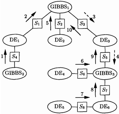
Now we complete the inward pass: the only universes in position to send active messages are the leaf uni­ verses DE2, DE4, and DE5. Assume that they send messages in that order. Next, DE6 absorbs the evi­ dence £o = (1, 0) and sends an active message to (the

DE universe) GIBBSg, which in turn sends one to DE3. Finally, DE3 sends an active message to GIBBS1, fin­ ishing the inward pass. Figure 3 illustrates the inward process, where solid arrows indicate active messages, dashed arrows indicate non-active cascade messages, and the labels attached to the arrows indicate the or­ der in which the messages were sent.

Having finished inward message passing in the hybrid junction tree, all universes will be of type DE; thus, outward message passing in a hybrid junction tree is performed as in conventional DE-type trees.

9 DISCUSSION

For illustration purposes the message scheduling in our example made a GIBBS universe send the first mes­ sage. In general, however, this will probably be sub­ optimal, since, as mentioned above, the more infor­ mation available before sampling takes place the bet­ ter. Thus, an optimal message scheduling strategy will probably select DE universes whenever possible. Thus, in our example a better schedule would probably let DE2, DE4, DEs, and DE6 send messages before either GIBBS2 or GIBBS3 send the next message.

As an indication of the anticipated ratio between the numbers of GIBBS and DE universes, we have investigated a subnetwork of the MUNIN network

(Andreassen, Jensen, Andersen, Falck, Kjrerulff, Woldbye, S0rensen, Rosenfalck & Jensen 1989) con­ sisting of 1041 nodes and 876 universes in a corre­ sponding junction tree. Letting all universes with ta­ bles containing more than 100, 000 entries be GIBBS universes, we find that 41 of the 876 universes should be of type GIBBS. The tables of these universes (con­ stituting less than 5% of the universes) take up 91.7% of the total storage engaged by universe tables. As­ suming that we generate 10, 000 samples in each of the 41 GIBBS universes, we still face a reduction of storage requirement by almost 90%. In absolute values, this means a reduction from 66 Mbytes to 7 Mbytes, using 32-bit representation of floating point numbers.

Experience shows that the ratio between the number of 'very large' universes and the number of 'smaller' universes in the above example is typical. That is, a small number of universes take up the majority of the total storage engaged. Thus, to obtain a large reduc­ tion of storage requirement, only a small proportion of the universes need to be of type GIBBS.

Supposedly, the present paper represents the very first attempt to combine exact and approximate inference in Bayesian networks. So, obviously, a large number of theoretical as well as practical issues need to be ad­ dressed. On the practical side, a thorough comparison with standard Gibbs and exact methods, will be con­ ducted in the very near future.

Regarding theoretical work, a large number of issues can be addressed. A few important ones are develop­ ment of methods providing variance estimates of the posteriors, development of methods to handle various kinds of continuous distributions, and development of alternative sampling schemes.

Acknowledgements

I am imdebted to my co-authors, A. Philip Dawid and Steffen L. Lauritzen, for providing the foundation of the present paper in the paper of Dawid et al. (1994). Further, I grateful to Steffen L. Lauritzen and anony­ mous referees for providing valuable comments on ear­ lier drafts of the paper. Finally, I thank the remaining members of the ODIN group at Aalborg University (http:/ fwww.iesd.auc.dkfodin) for providing a stimu­ lating environment. This research was supported by the Danish Research Councils through the PIFT pro­ gramme.

References

• Andersen, S. K., Olesen, K. G., Jensen, F. V. & Jensen, F. (1989). HUGIN- A shell for building Bayesian belief universes for expert systems, Pro-
• ceedings of the Eleventh International Joint Con­ ference on Artificial Intelligence, pp. 1080-1085.
• Andreassen, S., Jensen, F. V., Andersen, S. K., Falck, B., Kjrerulff, U., Woldbye, M., S0rensen, A. R., Rosenfalck, A. & Jensen, F. (1989). MUNIN - an expert EMG assistant, in J. E. Desmedt (ed.), Computer-Aided Electromyography and Ex­ pert Systems, Elsevier Science Publishers B. V. (North-Holland), Amsterdam, chapter 21.
• Dawid, A. P. (1992). Applications of a general propa­ gation algorithm for probabilistic expert systems, Statistics and Computing 2: 25-36.
• Dawid, A. P., Kjrerulff, U. & Lauritzen, S. L. (1994). Hybrid propagation in junction trees, Proceedings of the Fifth International Conference on Informa­ tion Processing and Management of Uncertainty in Knowledge-Based Systems (IPMU), Cite Inter­ nationale Universitaire, Paris, pp. 965-971.
• Geman, S. & Geman, D. (1984). Stochastic relaxation, Gibbs distributions, and the Bayesian restoration of images, IEEE Transactions on Pattern Analy­ sis and Machine Intelligence 6(6): 721-741.
• Jensen, C. S., Kong, A. & Kjrerulff, U. (1995). Blocking-Gibbs sampling in very large proba­ bilistic expert systems, International Journal of Human-Computer Studies. Special Issue on Real­ World Applications of Uncertain Reasoning. To appear.
• Jensen, F. V. (1988). Junction trees and decompos­ able hypergraphs, Research report, Judex Data­ systemer A/S, Aalborg, Denmark.
• Jensen, F. V., Lauritzen, S. L. & Olesen, K. G. (1990). Bayesian updating in causal probabilistic networks by local computations, Computational Statistics Quarterly 4: 269-282.
• Lauritzen, S. L. & Spiegelhalter, D. J. (1988). Lo­ cal computations with probabilities on graphical structures and their application to expert sys­ tems, Journal of the Royal Statistical Society, Se­ ries B 50(2): 157-224.
• Thomas, A., Spiegelhalter, D. J. & Gilks, W. R. (1992). BUGS: A program to perform Bayesian inference using Gibbs sampling, in J. M. Bernardo, J. 0. Berger, A. P. Dawid & A. F. M. Smith (eds), Bayesian Statistics 4, Oxford Uni­ versity Press, Oxford, UK, pp. 837-842.