HyFlex: A Benchmark Framework for Cross-domain Heuristic Search

Edmund Burke · Tim Curtois · Matthew

Hyde · Gabriela Ochoa · Jos´ e A. V´ azquez-Rodr´ ıguez

Received: date / Accepted: date

Abstract Automating the design of heuristic search methods is an active research field within computer science, artificial intelligence and operational research. In order to make these methods more generally applicable, it is important to eliminate or reduce the role of the human expert in the process of designing an effective methodology to solve a given computational search problem. Researchers developing such methodologies are often constrained on the number of problem domains on which to test their adaptive, self-configuring algorithms; which can be explained by the inherent difficulty of implementing their corresponding domain specific software components.

This paper presents HyFlex , a software framework for the development of crossdomain search methodologies. The framework features a common software interface for dealing with different combinatorial optimisation problems, and provides the algorithm components that are problem specific. In this way, the algorithm designer does not require a detailed knowledge the problem domains, and thus can concentrate his/her efforts in designing adaptive general-purpose heuristic search algorithms. Four hard combinatorial problems are fully implemented (maximum satisfiability, one dimensional bin packing, permutation flow shop and personnel scheduling), each containing a varied set of instance data (including real-world industrial applications) and an extensive set of problem specific heuristics and search operators. The framework forms the basis for the first International Cross-domain Heuristic Search Challenge (CHeSC), and it is currently in use by the international research community. In summary, HyFlex represents a valuable new benchmark of heuristic search generality, with which adaptive cross-domain algorithms are being easily developed, and reliably compared.

Keywords hyper-heuristics · combinatorial optimisation · search methodologies, self-adaptation, adaptation

Automated Scheduling, Optimisation and Planning (ASAP) research group

University of Nottingham, School of Computer Science,

Jubilee Campus, Wollaton Road, Nottingham NG8 1BB, UK

E-mail: { ekb,tec,mvh,gxo } @cs.nott.ac.uk

1 Introduction

There is a renewed and growing research interest in techniques for automating the design of heuristic search methods. The goal is to remove or reduce the need for a human expert in the process of designing an effective algorithm to solve a search problem, and consequently raise the level of generality at which search methodologies can operate. Evolutionary algorithms and metaheuristics have been successfully applied to solve a variety of real-world complex optimisation problems. Their design, however, has become increasingly complex. In order to make these methodologies widely applicable, it is important to provide self-managed systems that can configure themselves 'on the fly'; adapting to the changing problem (or search space) conditions, based on general high-level guidelines provided by their users.

Researchers pursuing these goals within combinatorial optimisation, are often limited by the number of problems domains available to them for testing their adaptive methodologies. This can be explained by the difficulty and effort required to implement state-of-the-art software components, such as the problem model, solution representation, objective function evaluation and search operators; for many different combinatorial optimisation problems. Although several benchmark problems in combinatorial optimisation are available (Taillard, 1993; Argelich et al, 2009; ESICUP, 2011; Beasley, 2010; TSPLIB, 2008) (to name just a few); they contain mainly the data of a set of instances and their best known solutions. They generally do not incorporate the software necessary to encode the solutions and calculate the objective function, let alone existing search operators for the given problem. It is the researcher who needs to provide these in order to later test their high-level adaptive search method. To overcome such limitations, we propose HyFlex , a modular and flexible Java class library for designing and testing iterative heuristic search algorithms. It provides a number of problem domain modules, each of which encapsulates the problem-specific algorithm components: solution representation, fitness evaluation, instance data, and a repository of associated problem-specific heuristics. Importantly, only the high-level control strategy needs to be implemented by the user, as HyFlex provides an easy to use interface with which the problem domains can be accessed. Indeed, HyFlex can be considered as an extension of the notion of a benchmark for combinatorial optimisation. Instead of providing only a data-set for a given problem domain, HyFlex also provides the problem specific software surrounding it. Thus, HyFlex acts as a benchmark for cross-domain optimisation and more general search methodologies.

A number of techniques and research themes within operational research, computer science and artificial intelligence would benefit from the proposed framework. Among them: hyper-heuristics (Burke et al, 2003b,a, 2010c; Ross, 2005), adaptive memetic algorithms (Krasnogor and Smith, 2001; Jakob, 2006; Ong et al, 2006; Smith, 2007; Neri et al, 2007), adaptive operator selection (Fialho et al, 2008, 2010; Maturana and Saubion, 2008; Maturana et al, 2010), reactive search (Battiti, 1996; Battiti et al, 2009), variable neighborhood search (Mladenovic and Hansen, 1997) and its adaptive variants (Braysy, 2002; Pisinger and Ropke, 2007); and generally the development of adaptive parameter control strategies in evolutionary algorithms (Eiben et al, 2007; Lobo et al, 2007). HyFlex can be seen, then, as a unifying benchmark, with which the performance of different adaptive techniques can be reliably assessed and compared. Indeed, HyFlex is currently used to support an international research competition: the First CrossDomain Heuristic Search Challenge (CHeSC, 2011). The challenge is analogous to the athletics Decathlon event, where the goal is not to excel in one event at the expense

of others, but to have a good general performance on each. The competition will also provide a set of state-of-the-art initial results on the HyFlex benchmark. Competitors will submit one Java class file representing their hyper-heuristic or high-level search strategy. This class file will then be run in HyFlex through the common interface. This ensures that the competition is fair, because all of the competitors must use the same problem representation and search operators. Moreover, due to the common interface, the competition will consider not only hidden instances, but also hidden domains. An interesting feature of CHeSC is the Leaderboard, a table which ranks participants according to their best score on a rehearsal competition conducted every week. This rehearsal competition is based on a set of results submitted by the participants who chose to do so. It has brought substantial dynamism and interest to the challenge. CHeSC currently has 43 registered teams from 23 different countries.

This article is structured as follows. Section 2 describes the antecedents and architecture of the HyFlex framework. It also includes examples of how to implement and run hyper-heuristics within the framework. Section 3 presents the four problem domains which are currently implemented: maximum satisfiability (MAX-SAT), onedimensional bin packing, permutation flow shop, and personnel scheduling. For each domain, details are given on the instance data, solution initialisation method, objective function evaluation, and the set of problem specific heuristics. Section 4 illustrates the implementation of three high-level search strategies using HyFlex: an iterative hyperheuristic, a multiple neighbourhood iterated local search algorithm, and a multi-meme memetic algorithm. They are not intended to be state-of-the-art adaptive approaches in their categories. Instead, they were selected to illustrate the wide range of algorithm designs that can be implemented within HyFlex. Section 5 presents a comparative study of the three algorithms. The goal is not to determine the best performing algorithm, but instead to illustrate their difference in behavior across the different problem domains. Finally, section 6 summarises our contribution and suggests directions for future research.

2 The HyFlex Framework

2.1 Overview of HyFlex

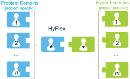
HyFlex (Hyper-heuristics Flexible framework) is a software framework designed to enable the development, testing and comparison of iterative general-purpose heuristic search algorithms (such as hyper-heuristics). To achieve these goals it uses modularity and the concept of decomposing a heuristic search algorithm into two main parts (see Figure 1):

1. A general-purpose part: the algorithm or hyper-heuristic.
2. The problem-specific part: provided by the HyFlex framework.

In the hyper-heuristics literature, this idea is also referred to as the domain barrier between the problem-specific heuristics and the hyper-heuristic (Burke et al, 2003a; Cowling et al, 2000). HyFlex extends the conceptual domain-barrier framework by maintaining a population (instead of a single incumbent solution) in the problem domain layer. Moreover, a richer variety of problem specific heuristics and search operators is provided. Another relevant antecedent to HyFlex is PISA (Bleuler et al, 2003),

a text-based software interface for multi-objective evolutionary algorithms. PISA provides a division between the application-specific and the algorithm-specific parts of a multi-objective evolutionary algorithm. In HyFlex, the interface is not text-based. Instead, it is given by an abstract Java class. This allows a more tight coupling between the modules and overcomes some of the speed limitations encountered in PISA. While PISA is designed to implement evolutionary algorithms, HyFlex can be used to implement both population-based and single point metaheuristics and hyper-heuristics. Moreover, it provides a rich variety of fully implemented combinatorial optimisation problems including real-world instance data.

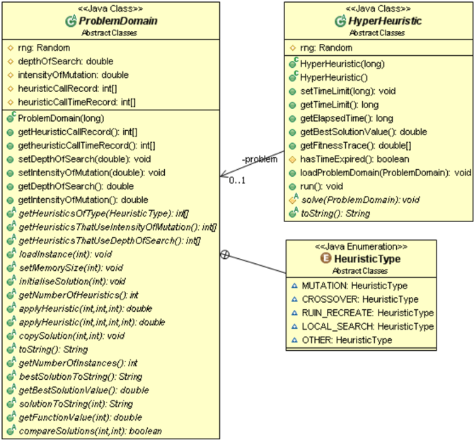
The framework is written in java which is familiar to and commonly used by many researchers. It also benefits from object orientation, platform independence and automatic memory management. At the highest level the framework consists of just two abstract classes: ProblemDomain and HyperHeuristic. The structure of these classes is shown in the class diagram of figure 2. In the diagram, the signatures adjacent to circles are public methods and fields, and the signatures adjacent to diamonds are protected. Abstract methods are denoted by italics, and the implementations of these methods are necessarily different for each problem domain class.

2.1.1 The ProblemDomain Class

As shown in figure 2, an implementation of the ProblemDomain class provides the following elements, each of which is easily accessed and managed with one or more methods.

1. A user-configurable memory (a population) of solutions, which can be managed by the hyper-heuristic through methods such as setMemorySize and copySolution .
2. A routine to randomly initialise solutions, initialiseSolution( i ) , where i is the index of the solution index in the memory.

2.1.2 Description

Problem formulation : 'SAT' refers to the boolean satisfiability problem. This problem involves determining if there is an assignment of the boolean variables

Table 1 MAX-SAT instances

	name	source	variables	clauses
1	contest02-Mat26.sat05-457.reshuffled-07	CRIL (2007)	744	2464
2	hidden-k3-s0-r5-n700-01-S2069048075.sat05-488.reshuffled-07	CRIL (2007)	700	3500
3	hidden-k3-s0-r5-n700-02-S350203913.sat05-486.reshuffled-07	CRIL (2007)	700	3500
4	parity-games/instance-n3-i3-pp	CRIL (2009)	525	2276
5	parity-games/instance-n3-i3-pp-ci-ce	CRIL (2009)	525	2336
6	parity-games/instance-n3-i4-pp-ci-ce	CRIL (2009)	696	3122
7	highgirth/3SAT/HG-3SAT-V250-C1000-1	Argelich et al (2009)	250	1000
8	highgirth/3SAT/HG-3SAT-V250-C1000-2	Argelich et al (2009)	250	1000
9	highgirth/3SAT/HG-3SAT-V300-C1200-2	Argelich et al (2009)	300	1200
10	MAXCUT/SPINGLASS/t7pm3-9999	Argelich et al (2009)	343	2058

of a formula, which results in the whole formula evaluating to true. If there is such an assignment then the formula is said to be satisfiable, and if not then it is unsatisfiable. An example formula is given in equation 2, which is satisfied when x 1 = false x 2 = false x 3 = true and x 4 = false .

HyFlex implements one of SAT's related optimisation problems, the maximum satisfiability problem (MAX-SAT), in which the objective is to find the maximum number of clauses of a given Boolean formula that can be satisfied by some assignment. The problem can also be formulated as a minimisation problem, where the objective is to minimise the number of unsatisfied clauses.

Solution initialisation : The solutions are initialised by randomly assigning a true or false value to each variable.

Objective function : The fitness function returns the number of 'broken' clauses, which are those which evaluate to false.

Instance data : The ten training instances and their sources are summarised in Table 2.

2.1.3 Search Operators

This domain contains a total of 9 search operators, summarised by Fukunaga (2008). Before describing them, find below four relevant definitions. Let T be the state of the formula before the variable is flipped, and let T ′ be the state of the formula after the variable is flipped.

• Net gain of a variable is defined as the number of broken clauses in T minus the number of broken clauses in T ′ .
• Positive gain of a variable is the number of broken clauses in T that are satisfied in T ′ .
• Negative gain of a variable is the number of satisfied clauses in T that are broken in T ′ .
• Age of a variable is the number of variable flips since it was last flipped.

Mutational heuristics

• h 1 : GSAT: Flip the variable with the highest net gain, and break ties randomly (Selman et al, 1992).

• h 2 : HSAT: Identical functionality to GSAT, but ties are broken by selecting the variable with the highest age (Gent and Walsh, 1993).
• h 3 : WalkSAT: Select a random broken clause BC. If any variables in BC have a negative gain of zero, randomly select one of these to flip. If no such variable exists, flip a random variable in BC with probability 0.5, otherwise flip the variable with minimal negative gain (Selman et al, 1994).
• h 4 : Novelty: Select a random broken clause BC. Flip the variable v with the highest net gain, unless v has the minimal age in BC. If this is the case, then flip it with 0.3 probability. Otherwise flip the variable with the second highest net gain (McAllester et al, 1997).

Ruin-recreate heuristics

h 5 : A proportion of the variables is randomly reinitialised.

Local search heuristics

• h 6 : This is a first-improvement local search. In each iteration, flip a variable selected completely at random.
• h 7 : This is a first-improvement local search. In each iteration, flip a randomly selected variable from a randomly selected broken clause.

Crossover heuristics

h 8 : Standard one point crossover on the boolean strings of variables.

h 9 : Standard two point crossover on the boolean strings of variables.

1. A set of problem specific heuristics, which are used to modify solutions. These are called by the user's hyper-heuristic with the applyHeuristic( i, j, k ) method, where i is the index of the heuristic to call, j is the index of the solution in memory to modify, and k is the index in memory where the resulting solution should be put. Each problem-specific heuristic in each problem domain is classified into one of four groups, shown below. The heuristics belonging to a specific group can be accessed by calling getHeuristicsOfType( type ) .
2. -Mutational or perturbation heuristics: perform a small change on the solution, by swapping, changing, removing, adding or deleting solution components.
3. -Ruin-recreate (destruction-construction) heuristics: partly destroy the solution and rebuild or recreate it afterwards. These heuristics can be considered as large neighbourhood structures. They are, however, different from the mutational heuristics in that they can incorporate problem specific construction heuristics to rebuild the solutions
4. -Hill-climbing or local search heuristics: iteratively make small changes to the solution, only accepting non-deteriorating solutions, until a local optimum is found or a stopping condition is met. These heuristics differ from mutational heuristics in that they incorporate an iterative improvement process, and they guarantee that a non-deteriorating solution will be produced.
5. -Crossover heuristics: take two solutions, combine them, and return a new solution.
6. Avaried set of instances that can be easily loaded using the method loadInstance( a ) , where a is the index of the instance to be loaded.
7. A fitness function, which can be called with the getFunctionValue( i ) method, where i is the index of the required solution in the memory. HyFlex problem domains are always implemented as minimisation problems, so a lower fitness is always superior. The fitness of the best solution found so far in the run can be obtained with the getBestSolutionValue() method.

1. Two parameters: α and β, (0 < = [ α, β ] < = 1), which are the 'intensity' of mutation and 'depth of search', respectively, that control the behaviour of some search operators.

2.1.4 The HyperHeuristic Class

The HyperHeuristic class is designed to allow algorithms which implement this class to be compared and benchmarked across one or more of the problem domains available (for example, in a competition). Users create cross-domain heuristic algorithms by creating implementations of this abstract class. Each class must contain a toString() method, to give the methodology a name. It must also contain a solve() method, in which the functionality of the particular methodology is written.

The solve() method would normally contain a loop, which continues while the time limit (defined by the user) has not been exceeded. In the loop, the code should provide a mechanism for selecting between the available problem-specific heuristics, and choose to which solutions in memory to apply the heuristics. This class could choose to work with a memory size of 1 for a single point search, or a large memory could be maintained for a population based approach. The memory can be easily defined and

maintained through calling methods of the ProblemDomain class, where the memory is stored. A hyper-heuristic class automatically records the length of time for which it has been running, and this can be monitored through methods such as hasTimeExpired() and getElapsedTime() .

The solve method is the only method which must be implemented, all other common functionality is provided by the HyFlex software, such as the timing function and the recording of the best solution.

2.2 Running a Hyper-Heuristic

Algorithm 1 shows the ease with which a hyper-heuristic can be run on a problem domain. An object is created for the problem domain (in this example MAX-SAT), and for the hyper-heuristic, each with a random seed. Then a problem instance is loaded from the selection available in the problem domain object. In this example we choose the instance with index 0. The problem domain is now set up for the hyper-heuristic.

We set the time for which the hyper-heuristic will run, in milliseconds. Then the hyper-heuristic object is given a reference to the problem domain object. Now that the setup is complete, the run() method of the hyper-heuristic is called, to start the search process. The hyper-heuristic will run for 60 seconds in this example, and the best solution found during that time is retrievable with the getBestSolutionValue() method, as shown in algorithm 1.

Algorithm 1 Java code for running a hyper-heuristic on a problem domain
ProblemDomain problem = new SAT(1234); HyperHeuristic HHObject = new problem.loadInstance(0); HHObject.setTimeLimit(60000); HHObject.loadProblemDomain(problem); HHObject.run(); System.out.println(HHObject.getBestSolutionValue());
ExampleHyperHeuristic1(5678);

2.3 An Example Hyper-Heuristic

This section provides an example hyper-heuristic, to illustrate the ease with which a hyper-heuristic can be created. This is done by extending the HyperHeuristic abstract class, and implementing only one method. All of the common functionality is provided by the HyFlex software, such as the timing function and the recording of the best solution. This example demonstrates exactly how to use certain elements of HyFlex functionality, including the solution memory.

After the run() method of the hyper-heuristic is called (see section 2.2), the hyperheuristic abstract class performs some housekeeping tasks, such as initialising the timer, and then calls the solve method of the chosen hyper-heuristic. In our example this is an object of the class ExampleHyperHeuristic1 . Algorithm 2 shows the code for the solve() method in ExampleHyperHeuristic1 . It shows that very few lines of code are

necessary in order to implement a hyper-heuristic method with the HyFlex framework. Algorithm 2 is written in pseudocode, but each line corresponds to no more than one line of actual Java code. The solve() method is the only substantial method which needs to be implemented. Indeed the only other necessary method is toString() , which requires one line to give the hyper-heuristic a name.

From Algorithm 2, we can see that the solve() method takes the problem domain object as an argument, and first checks for the number of search operators available within it. We also initialise a value to store the current objective function value. It is also necessary to initialise at least one solution in the memory. The default memory size is 2, and we initialise the solution at index 0, which means we build an initial solution with the method specified in the problem domain (generally a fast randomised constructive heuristic). The solution at index 1 remains uninitialised, and therefore has a value of null .

An implemented hyper-heuristic must always contain a while loop which checks if the time limit has expired. The code within the loop specifies the main functionality of the hyper-heuristic. In this example, we choose a random operators, and then apply it to the solution at index 0. The modified solution is put in the memory at index 1 (previously not initialised). Note that a random number generator rng is provided by the HyperHeuristic abstract class. This is created when the hyper-heuristic object's constructor is called, and is the reason why that constructor requires a random seed.

If the new solution is superior to the old solution, it is accepted, and the new solution overwrites the old one in memory. The copySolution method of the problem domain class is employed to manage this. If the new solution is not superior, then the new solution is accepted with 0.5 probability.

Algorithm 2 Pseudocode for the solve method of ExampleHyperHeuristic1 . This is called when the run() method of the hyper-heuristic is called (see algorithm 1)

Require: A ProblemDomain object, problem int numberOfHeuristics = problem.getNumberOfHeuristics double currentObjValue = Double.POSITIVE-INFINITY problem.initialiseSolution(0) while hasTimeExpired = FALSE do int h = rng.nextInt(numberOfHeuristics) double newObjValue = problem.applyHeuristic(h, 0, 1) double delta = currentObjValue - newObjValue if delta > 0 then problem.copySolution(1, 0) currentObjValue = newObjValue; else if rng.nextBoolean = TRUE then problem.copySolution(1, 0) currentObjValue = newObjValue; end if end if

end while

2.4 Summary of HyFlex Description

In this section, we have given an overview of the HyFlex framework, and demonstrated that it is very easy to create and run a hyper-heuristic using the framework. The contribution of HyFlex is that the hyper-heuristic developer now does not need expertise in any of the problem domains. The developer is therefore free to focus their research efforts into developing hyper-heuristic methodologies which can be shown to be generally successful across a range of problem domains.

3 HyFlex Problem Domains

Currently, four problem domain modules are implemented(which can be downloaded from CHeSC (2011)): maximum satisfiability (MAX-SAT), one-dimensional bin packing, permutation flow shop, and personnel scheduling. Each domain includes 10 training instances from different sources, and number of problem-specific heuristics of the types discussed in section 2.1.

3.1 Maximum Satisfiability (MAX-SAT)

3.1.1 Description

Problem formulation : 'SAT' refers to the boolean satisfiability problem. This problem involves determining if there is an assignment of the boolean variables of a formula, which results in the whole formula evaluating to true. If there is such an assignment then the formula is said to be satisfiable, and if not then it is unsatisfiable. An example formula is given in equation 2, which is satisfied when x 1 = false x 2 = false x 3 = true and x 4 = false .

HyFlex implements one of SAT's related optimisation problems, the maximum satisfiability problem (MAX-SAT), in which the objective is to find the maximum number of clauses of a given Boolean formula that can be satisfied by some assignment. The problem can also be formulated as a minimisation problem, where the objective is to minimise the number of unsatisfied clauses.

Solution initialisation : The solutions are initialised by randomly assigning a true or false value to each variable.

Objective function : The fitness function returns the number of 'broken' clauses, which are those which evaluate to false.

Instance data : The ten training instances and their sources are summarised in Table 2.

3.1.2 Search Operators

This domain contains a total of 9 search operators, summarised by Fukunaga (2008). Before describing them, find below four relevant definitions. Let T be the state of the formula before the variable is flipped, and let T ′ be the state of the formula after the variable is flipped.

Table 2 MAX-SAT instances

	name	source	variables	clauses
1	contest02-Mat26.sat05-457.reshuffled-07	CRIL (2007)	744	2464
2	hidden-k3-s0-r5-n700-01-S2069048075.sat05-488.reshuffled-07	CRIL (2007)	700	3500
3	hidden-k3-s0-r5-n700-02-S350203913.sat05-486.reshuffled-07	CRIL (2007)	700	3500
4	parity-games/instance-n3-i3-pp	CRIL (2009)	525	2276
5	parity-games/instance-n3-i3-pp-ci-ce	CRIL (2009)	525	2336
6	parity-games/instance-n3-i4-pp-ci-ce	CRIL (2009)	696	3122
7	highgirth/3SAT/HG-3SAT-V250-C1000-1	Argelich et al (2009)	250	1000
8	highgirth/3SAT/HG-3SAT-V250-C1000-2	Argelich et al (2009)	250	1000
9	highgirth/3SAT/HG-3SAT-V300-C1200-2	Argelich et al (2009)	300	1200
10	MAXCUT/SPINGLASS/t7pm3-9999	Argelich et al (2009)	343	2058

• Net gain of a variable is defined as the number of broken clauses in T minus the number of broken clauses in T ′ .
• Positive gain of a variable is the number of broken clauses in T that are satisfied in T ′ .
• Negative gain of a variable is the number of satisfied clauses in T that are broken in T ′ .
• Age of a variable is the number of variable flips since it was last flipped.

Mutational heuristics

• h 1 : GSAT: Flip the variable with the highest net gain, and break ties randomly (Selman et al, 1992).
• h 2 : HSAT: Identical functionality to GSAT, but ties are broken by selecting the variable with the highest age (Gent and Walsh, 1993).
• h 3 : WalkSAT: Select a random broken clause BC. If any variables in BC have a negative gain of zero, randomly select one of these to flip. If no such variable exists, flip a random variable in BC with probability 0.5, otherwise flip the variable with minimal negative gain (Selman et al, 1994).
• h 4 : Novelty: Select a random broken clause BC. Flip the variable v with the highest net gain, unless v has the minimal age in BC. If this is the case, then flip it with 0.3 probability. Otherwise flip the variable with the second highest net gain (McAllester et al, 1997).

Ruin-recreate heuristics

• h 5 : A proportion of the variables is randomly reinitialised.

Local search heuristics

• h 6 : This is a first-improvement local search. In each iteration, flip a variable selected completely at random.
• h 7 : This is a first-improvement local search. In each iteration, flip a randomly selected variable from a randomly selected broken clause.

Crossover heuristics

• h 8 : Standard one point crossover on the boolean strings of variables.
• h 9 : Standard two point crossover on the boolean strings of variables.

3.2 One Dimensional Bin Packing

3.2.1 Description

Problem formulation : The classical one dimensional bin packing problem consists of a set of pieces, which must be packed into as few bins as possible. Each piece j has a weight w j , and each bin has capacity c . The objective is to minimise the number of bins used, where each piece is assigned to one bin only, and the weight of the pieces in each bin does not exceed c . To avoid large plateaus in the search space around the best solutions, we employ an alternative fitness function to the number of bins. A mathematical formulation of the bin packing problem is shown in equation 3, taken from (Martello and Toth, 1990).

Where y i is a binary variable indicating whether bin i contains pieces, x ij indicates whether piece j is packed into bin i , and n is the number of available bins (and also the number of pieces as we know we can pack n pieces into n bins).

Solution initialisation : Solutions are initialised by first randomising the order of the pieces, and then applying the 'first-fit' heuristic (Johnson et al, 1974). This is a constructive heuristic, which packs the pieces one at a time, each into the first bin into which they will fit.

Objective function : A solution is given a fitness calculated from equation 4, where: n = number of bins, fullness i = sum of all the pieces in bin i , and C = bin capacity. The function puts a premium on bins that are filled completely, or nearly so. It returns a value between zero and one, where lower is better, and a set of completely full bins would return a value of zero.

Instance data : The ten training instances and their sources are summarised in Table 3.

3.2.2 Search Operators

This domain contains a total of 8 search operators, some of which are taken from (Bai et al, 2007).

Mutational heuristics

Table 3 Bin packing instances

name	source	capacity	no. pieces
falkenauer/u1000-00	ESICUP (2011)	150	1000
falkenauer/u1000-01	ESICUP (2011)	150	1000
schoenfieldhard/BPP14	ESICUP (2011)	1000	160
schoenfieldhard/BPP832	ESICUP (2011)	1000	160
10-30/instance1	Hyde (2011)	150	2000
10-30/instance2	Hyde (2011)	150	2000
triples1002/instance1	Hyde (2011)	1000	1002
triples2004/instance1	Hyde (2011)	1000	2004
test/testdual4/binpack0	ESICUP (2011)	100	5000
test/testdual7/binpack0	ESICUP (2011)	100	5000

• h 1 : Select two different pieces at random, and swap them if there is space. If one of the pieces does not fit into the new bin then put it into an empty bin.
• h 2 : This heuristic selects a bin at random from those with more pieces than the average. It then splits this bin into two bins, each containing half of the pieces from the original bin.
• h 3 : Remove all of the pieces from the lowest filled bin, and repack them into the other bins if possible, with the best-fit heuristic.

Ruin-recreate heuristics

• h 4 : Remove all the pieces from the x highest filled bins, where x is an integer determined by the 'intensity of mutation' parameter. Repack the pieces using the best-fit heuristic.
• h 5 : Remove all the pieces from the x lowest filled bins, where x is an integer determined by the 'intensity of mutation' parameter. Repack the pieces using the best-fit heuristic.

Local search heuristics

These heuristics implement first-improvement local search operators. In each iteration, a neighbour is generated, and it is accepted immediately if it has superior or equal fitness. If the neighbour is worse, then the change is not accepted.

• h 6 : A first-improvement local search. In each iteration, select two different pieces at random, and swap them if there is space, and if it will produce an improvement in fitness.
• h 7 : A first-improvement local search. Take the largest piece from the lowest filled bin, and exchange with a smaller piece from a randomly selected bin. If there is no such piece that produces a valid packing after the swap, then exchange the first piece with two pieces that have a smaller total size. If there are no such pieces then the heuristic does nothing.

Crossover heuristics

• h 8 : Exon shuffling crossover (Rohlfshagen and Bullinaria, 2007). The bins from both parents are ordered by wasted space, least first. Then all of the mutually exclusive bins are added to the offspring. In the second phase, the remaining bins from the parents are added to the offspring by removing any duplicate pieces.

3.3 Permutation Flow Shop

3.3.1 Description

Problem formulation : The permutation flow shop problem consists of finding the order in which n jobs are to be processed in m consecutive machines. The jobs are processed in the order machine 1, machine 2, . . . , machine m . Machines can only process one job at a time and jobs can be processed by only one machine at a time. No job can jump over any other job, meaning that the order in which jobs are processed in machine 1 is maintained throughout the system. Moreover, no machine is allowed to remain idle when a job is ready for processing. All jobs and machines are available at time 0. Each job i requires a processing time on machine j denoted by p ij .

Given a permutation π = π (1) , . . . , π ( n ), where π ( q ) is the index of the job assigned in the q -th place, a unique schedule is obtained by calculating the starting and completion time of each job on each machine. The starting time start π ( q ) ,j of the q -th job on machine j is calculated as:

with

and its completion time is calculated as:

Given a schedule, let C i be the time when job i finishes its processing on machine m . The objective is to find the processing order of n jobs in such a way that the resultant schedule minimises the completion time of the last job to exit the shop, i.e. minimises max i C i .

Solution initialisation : Solutions are created with a randomised version of the widely used NEH algorithm (Nawaz et al, 1983), which works as follows. First a random permutation of the jobs is generated. Second, a schedule is constructed from scratch by assigning the first job in the permutation to an empty schedule; the second job is then assigned to places 1 and 2 and fixed where the partial schedule has the smallest makespan; the third job is assigned to places 1, 2 and 3 and fixed to the place where the partial schedule has the smallest makespan, and so on.

Objective function : The fitness function returns max i C i . Representing the completion time of the last job in the schedule.

Instance data : The ten training instances and their sources are summarised in Table 4.

3.3.2 Search Operators

A total of 15 search operators are implemented for this problem domain.

Mutational heuristics

• h 1 : Reinserts a randomly selected job into a randomly selected position in the permutation, shifting the rest of the jobs as required.
• h 2 : Swaps two randomly selected jobs in the permutation.
• h 3 : Randomly shuffles the entire permutation.

Table 4 Permutation flowshop instances

instance	name	source	no. jobs	no. machines
1	100x20/1	Taillard (2010)	100	20
2	100x20/2	Taillard (2010)	100	20
3	100x20/3	Taillard (2010)	100	20
4	100x20/4	Taillard (2010)	100	20
5	100x20/5	Taillard (2010)	100	20
6	200x10/2	Taillard (2010)	200	10
7	200x10/3	Taillard (2010)	200	10
8	500x20/1	Taillard (2010)	500	20
9	500x20/2	Taillard (2010)	500	20
10	500x20/4	Taillard (2010)	500	20

• h 4 : Creates a new solution using NEH (described above) and using the current permutation to rank the jobs.
• h 5 : Shuffles k randomly selected elements in the permutation, where k = 2 + glyph[floorleft] α · ( n -2) glyph[floorright] , and α is the mutation intensity parameter.

Ruin-recreate heuristics

• h 6 : Remove l , l = glyph[floorleft] α · ( n -1) glyph[floorright] , randomly selected jobs and reinsert them in an NEH fashion. This heuristic resembles the main component of the iterated greedy heuristic proposed by Ruiz and St¨ utzle. (2007b) for the permutation flow shop and later by Ruiz and St¨ utzle. (2007a) for the permutation flow shop with sequence dependent setup times.
• h 7 : Remove l , where l is as above, randomly selected jobs, reinsert them in an NEH fashion but this time, at every iteration of the NEH procedure the best q , q = glyph[floorleft] β · ( l -1) glyph[floorright] +1, sequences generated so far are considered for the reinsertion.

Local search heuristics

• h 8 : This is a steepest descent local search. At every iteration each job is removed from its current position and assigned into all remaining positions. The job is fixed to the position that leads to the best schedule. This is repeated until no improvement is observed.
• h 9 : This is a first improvement local search. At every iteration each job is removed from its current position and assigned into the remaining positions. This time, if an improvement movement is found, this is immediately accepted, and the search continues with the next job. This is repeated until no improvement is observed.
• h 10 : This is a random single local search pass. In this, r = glyph[floorleft] β ( n -1) glyph[floorright] +1 randomly selected jobs are tested (one at a time) on all positions and fixed to the best possible place. This is only done once.
• h 11 : This is a first improvement random single local search pass. This is as h 9 but jobs are assigned to the first place that improves the current schedule, i.e. jobs are not necessarily tested in all positions. This is only done once.
• Crossover heuristics The following crossover heuristics take two permutations as an input and return a single new permutation as offspring. These operators have been designed for permutation representation problems, including scheduling problems.
• h 13 : Partially mapped crossover (PMX): first proposed by Goldberg and Lingle (1985), as a recombination operator for the traveling salesman probem (TSP).

• It builds an offspring by choosing a subsequence of a tour from one parent and preserving the order and position of as many elements (cities in the case of TSP) as possible. A subsequence of a tour is selected by randomly choosing two cut points, which serves as boundaries for the swapping operations.
• h 12 : Order crossover (OX): proposed by Davis (1985) for order-based permutation problems. It builds an offspring permutation by choosing a subsequence of a solution from one parent and preserving the relative order of elements from the other parent. The OX operator exploits the property that the relative order of the elements (as opposed to their specific positions) is important.
• h 14 : Precedence preservative crossover (PPX): independently developed for the vehicle routing problems by Blanton and Wainwright (1993), and for scheduling problems by Bierwirth et al (1996). PPX transmits precedence relations of operations given in two parental permutations to one offspring at the same rate, while no new precedence relations are introduced.
• h 15 : This operators selects a single crossover point and produces a new permutation by copying all of the elements from one parent, up to the crossover point. Then the remaining elements are copied from the other parent, in the order that they appear.

3.4 Personnel Scheduling

3.4.1 Description

Problem formulation : Most of the personnel scheduling instances could justifiably be labelled as a new and different problem rather than just a different instance. This is because most instances contain unique constraints and objectives, not just different instance parameters (such as the number of employees, shift types, planning period length, constraint priorities etc). The reason for this variety is that each instance is taken from a different organisation or workplace and each workplace has its own set of rules and requirements. However, there is clearly a similar structure between instances and there are some constraints that are nearly always present. For example, cover constraints, holiday requests, maximum and minimum workloads etc. The result of this variety though is that it is arguably impossible to provide a standard mathematical model for 'The Personnel Scheduling Problem' and we will not attempt to do so here. However, for more information on the constraints and objectives present in the instances used here (and an integer programming formulation of one of them) we refer the reader to Curtois (2010).

Solution initialisation : The solution is initialised using local search heuristic h 5 which adds shifts to each employee's schedule in a greedy, first improvement manner. Instance data : The instances used are listed in Table 5.

3.4.2 Search Operators

A total of 12 search operators are implemented for this problem domain.

Mutational heuristics

• h 1 : This heuristic randomly un-assigns a number of shifts. The number of shifts un-assigned is proportional to the intensity of mutation parameter.

Table 5 Personnel scheduling instances

name		source staff	shift types	days
BCV-3.46.1	Curtois (2009)	46	3	26
BCV-A.12.2	Curtois (2009)	12	5	31
ORTEC02	Curtois (2009)	16	4	31
Ikegami-3Shift-DATA1	Ikegami and Niwa (2003)	25	3	30
Ikegami-3Shift-DATA1.1	Ikegami and Niwa (2003)	25	3	30
Ikegami-3Shift-DATA1.2	Ikegami and Niwa (2003)	25	3	30
CHILD-A2	Curtois (2009)	41	5	42
ERRVH-A	Curtois (2009)	51	8	42
ERRVH-B	Curtois (2009)	51	8	42
MER-A	Curtois (2009)	54	12	42

• Ruin-recreate heuristics The ruin and recreate heuristics implemented are based on the one presented by Burke et al (2008). The heuristic works by un-assigning all the shifts in one or more randomly selected employees' schedules before heuristically rebuilding them. They are rebuilt by firstly satisfying objectives related to requests to work certain days or shifts and then by satisfying objectives related to weekends. For example min/max weekends on/off, min/max consecutive working or non-working weekends, both days of the weekend on or off etc. Other shifts are then added to the employee's schedule in a greedy fashion (first improvement) attempting to satisfy the rest of the objectives.
• h 2 : Burke et al (2008) observed that it was best to un-assign and rebuild only 2-6 work patterns at a time (for instances of all sizes). For this reason the first ruin and recreate heuristic un-assigns x schedules where x is calculated using the intensity of mutation parameter as follows:
• h 3 : This heuristic provides a larger change to the solution by setting x using:
• x = Round(intensityOfMutation * Number of employees in roster)

x = Round(intensityOfMutation * 4) + 2

h 4 : This heuristic creates a small perturbation in the solution by using x = 1.

Local Search Heuristics

• h 5 : This is a first improvement local search which adds shifts to employees' schedules.
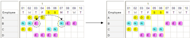
• h 6 : This is a first improvement local search which swaps shifts between two different employees. An example of the type of swap this local search may make is shown in Figure 3. The figure shows a section of a roster showing the the first ten days of the schedules for four employees: 'A', 'B', 'C' and 'D'. The coloured squares labelled 'D', 'E' and 'N' denote three different shifts types (Early, Day and Night)
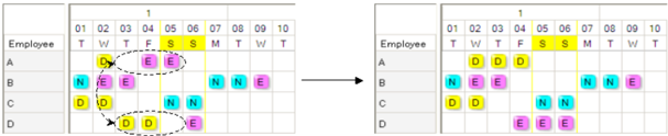
• h 7 : This is a first improvement local search which swaps shifts in a single employee's schedule. An example of the type of swap this local search may make is shown in Figure 4.
• h 8 : This is based on the ejection chain method described by Burke et al (2007). The maximum search time for it is set as: the depth of search parameter multiplied by 5 seconds.

h 9 : This is another version of the ejection chain method which incorporates a greedy heuristic method for generating entire schedules for single employees. The maximum search time for it is set as: the depth of search parameter multiplied by 5 seconds.

Crossover heuristics

h 10 : This heuristic was presented by Burke et al (2001). It operates by identifying the best x assignments in each parent and making these assignments in the offspring. The best assignments are identified by measuring the change in objective function when each shift is temporarily unassigned in the roster. The best assignments are those that cause the largest increase in the objective function value when they are unassigned. The parameter x ranges from 4-20 and is calculated using the intensity of mutation parameter as below:

x = 4 + round((1 -intensityOfMutation) * 16)

h 11 : This heuristic was published in (Burke et al, 2010b). It creates a new roster by using all the assignments made in the parents. It makes those that are common to both parents first and then alternately selects an assignment from each parent and makes it in the offspring unless the cover objective is already satisfied.

h 12 : This heuristic creates the new roster by making assignments which are only common to both parents.

4 Algorithms

This section presents three example algorithms created within the HyFlex software framework. We present these algorithms in order to show the range of algorithms that can be easily implemented in HyFlex. The results of these three algorithms are presented in section 5, to show the diversity of their results across the different problem

instances and problem domains. Recall from section 2.1.1 that HyFlex problem domains are always implemented as minimisation problems, so a lower fitness is superior.

4.1 Iterated Local Search

Iterated local search is a relatively straightforward algorithm. As often happens with many simple but sometimes very effective ideas, the same principle has been rediscovered multiple times, leading to different names (Baxter, 1981; Martin et al, 1992). The term iterated local search was proposed byLourenco et al (2002). The implementation reported here, first proposed in in (Burke et al, 2010a), contains a perturbation stage during which a neighborhood move is selected uniformly at random (from the available pool) and applied to the incumbent solution. This perturbation phase is then followed by an improvement phase, in which all local search heuristics are tested and the one producing the best improvement is used. If the resulting new solution is better than the original solution then it replaces the original solution, otherwise the new solution is simply discarded. This last stage corresponds to a greedy (only improvements) acceptance criterion. The pseudo-code of this iterated local search algorithm is shown below (Algorithm 3).

Algorithm 3 Iterated Local Search .
s 0 = GenerateInitialSolution s ∗ = LocalSearch( s 0 ) repeat s ′ = Perturbation ( s ∗ ) s ∗ ′ = LocalSearch( s ′ ) if f ( s ∗ ′ ) < f ( s ∗ ) then s ∗ = s ∗ ′ end if until time limit is reached

4.2 Tabu Search Hyper-heuristic with Adaptive Acceptance (TS-AA)

The functionality of this hyper-heuristic can be split into two parts, the heuristic selection mechanism and the move acceptance criteria. The pseudocode for TS-AA can be seen in Algorithm 4.

Heuristic selection mechanism for TS-AA : This hyper-heuristic implements the heuristic selection mechanism proposed in (Burke et al, 2003b).The algorithm maintains a value for each of the problem-specific heuristics, excluding the crossover type heuristics. The crossover heuristics are not used at all by this hyper-heuristic. The heuristic's value represents how well it has performed recently, and all heuristics have a value of zero at the beginning of the search. The mechanism also incorporates a dynamic tabu list of problem-specific heuristics that are temporarily excluded from the available heuristics.

At each iteration, the heuristic with the highest value is selected (breaking ties randomly), from those not in the tabu list. Therefore, the heuristics which have performed

well recently will be chosen more often. If the heuristic finds a better solution, then its value is increased. If it finds a worse solution, its value is decreased.

Acceptance criterion for TS-AA : The acceptance criterion accepts all improving solutions. Other solutions are accepted with a probability β . which changes depending on whether the search appears to be progressing or stuck in a local optimum. The β value begins at zero, thus, initially, it is an accept-only-improving strategy. However, if the solution does not improve for 0.1 seconds, then β is increased by 5%, making it more likely that a worse solution is accepted. It is increased to 10% if there is no further improvement in the next 0.1 seconds. Conversely, if the search is progressing well, with no decrease in fitness in the last 0.1 seconds, then β is reduced by 5%, making it less likely for a worse solution to be accepted. These modifications are intended to help the search navigate out of local optima, and to focus the search if it is progressing well.

4.3 Memetic Algorithm

This algorithm illustrates a population based approach implemented with HyFlex. It represents a steady-state evolutionary algorithm that incorporates multiple memes (a memetic algorithm). The pseudocode is given in Algorithm 5. First a population of 10 solutions is generated, each one initialised with the initialiseSolution() method provided by each problem domain. Two solutions are selected with a binary tournament method, and then a crossover type heuristic (selected uniformly at random from the available set) is applied to produce one offspring.

With 0.1 probability, the offspring is perturbed with a mutation heuristic (selected uniformly at random from the available set). Then the solution is further modified with either a local search heuristic or a ruin-recreate heuristic, chosen with a 0.5 probability (also selected each uniformly at random). If the new solution is equal to or better than the worst of the parents, then the offspring replaces it.

5 Experiments and Results

This section compares the three algorithms described in section 4 implemented with HyFlex. Exactly the same algorithms are used for each domain and instance. No domain-specific (or instance-specific) tuning process is applied. The goal is not to determine which is the best performing algorithm, but instead to illustrate the behaviour of different algorithmic designs in HyFlex. The 10 training instances for each domain, as described in section 2 (Tables 2-5), were considered. For each instance and algorithm, 5 runs were conducted, each lasting 10 CPU minutes. This experimental setup resembles that designed for the CHeSC competition. The experiments were conducted on a PC (running Windows XP) with a 2.33GHz Intel(R) Core(TM)2 Duo CPU and 2GB of RAM. The following subsections present our results from three different perspectives: ordinal data analysis (5.1), distribution of best objective function values on one selected instance per domain (5.2), performance behaviour over time on one example instance of the bin packing domain (5.3).

Create a initial solution s Initialise the value of each heuristic to 0 α = 1 β = 0 t = tabu tenure = number of heuristics-1 repeat Create a copy of the current solution: s ′ ← s H = heuristic with highest value apply H to s ′ if func ( s ′ ) < func ( s ) then { the new solution is superior } increaseV alue ( H,α ) else if func ( s ′ ) < func ( s ) then { the new solution is worse } empty the tabu list decreaseV alue ( H,α ) add H to the tabu list else if func ( s ′ ) = func ( s ) then add H to the tabu list release heuristics in tabu list for longer than t iterations end if if func ( s ′ ) < func ( s ) then s ← s ′ else if random [1 , 100] < β then s ← s ′ end if end if if 0.1s since last improvement then { make it more likely to accept worse solutions } β ← β +5 end if if 0.1s since last decrease in fitness then { make it less likely to accept worse solutions } β ← β -5 end if until time limit is reached

5.1 Borda count

Ordinal data analysis methods can be applied to compare alternative search algorithms or metaheuristics (Talbi, 2009). This approach is adequate because our empirical study considers different domains and instances with varied magnitudes and ranges of the objective values. Let us assume that m instances (considering all the domains) and n competing algorithms in total are considered. For each experiment (instance) an ordinal value o k is given representing the rank of the algorithm compared to the others (1 ≤ o k ≤ n ). Ordinal methods aggregate and summarise m linear orders o k into a single linear order O . We use here a straight forward ordinal aggregation method know as the Borda count voting method (after the French mathematician Jean-Charles de

Algorithm 5 Memetic algorithm

population = Create a initial population of 10 solutions repeat s1 = binaryTournament(population); s2 = binaryTournament(population); h = randomly selected crossover heuristic s ′ = applyheuristic( h , s1, s2); Apply randomly selected mutation heuristic to s ′ if rand < 0 . 5 then h = randomly selected local search heuristic else h = randomly selected ruin-recreate heuristic end if applyheuristic( h , s ′ ); if f ( s 1) worse than f ( s 2) then s 1 ← s ′ else s 2 ← s ′ end if until time limit is reached

Table 6 Borda count results for all domains

Domain	TS-AA	ILS	MA
MAX-SAT	12	27	21
1D Bin Packing	24	17	19
Permutation Flow Shop	30	17	13
Personnel Scheduling	13	16	30
Total	79	77	83

Borda, who first proposed it in 1770). An algorithm having a rank o k in a given instance is simply given o k points, and the total score of an algorithm is the sum of its ranks o k across the m instances. The methods are, therefore, compared according to their total score, with the smallest score representing the best performing algorithm. In our comparative study, the number of instances, m , is 40 (10 for each domain). Therefore, for a given domain the best possible score is 10, while the best possible total score (considering all the domains) is 40. The ranks were calculated using as a metric the median of the best objective functions obtained across the 5 runs per instance.

Table 6 shows the total Borda scores for the three competing algorithms, including the total scores per domain. Notice that although TS-AA produces the best scores in two domains: MAX-SAT and permutation flow shop; the ILS algorithm obtains the best overall scores, although by a minimal difference. Tables 7-10 show the Borda count (ranks) for each instance on the four domains, where 1 represents the best rank. These tables are useful to assess how homogeneous the results are for the ten instances on each domain. For example, for permutation flow shop and personnel scheduling (Tables 9-10) a single algorithm is consistently ranking 3rd, whereas this is not the case for MAX-SAT and bin packing (Tables 7-8).

Table 7 Borda count results for MAXSAT

MAX-SAT	TS-AA	ILS	MA
Instance1	2	3	1
Instance2	2	3	1
Instance3	1	3	2
Instance4	1	2	3
Instance5	1	2	3
Instance6	1	2	3
Instance7	1	3	2
Instance8	1	3	2
Instance9	1	3	2
Instance10	1	3	2
Total	12	27	21

Table 9 Borda count results for permutation flowshop

Table 8 Borda count results for 1D Bin Packing

Bin Packing	TS-AA	ILS	MA
Instance1	3	1	2
Instance2	3	1	2
Instance3	3	2	1
Instance4	2	3	1
Instance5	2	1	3
Instance6	3	1	2
Instance7	3	1	2
Instance8	3	1	2
Instance9	1	3	2
Instance10	1	3	2
Total	24	17	19

Table 10 Borda count results for personnel scheduling

Flow Shop	TS-AA	ILS	MA	Personnel Sched.	TS-AA	ILS	MA
Instance1	3	2	1	Instance1	1	2	3
Instance2	3	1	2	Instance2	2	1	3
Instance3	3	2	1	Instance3	1	1	3
Instance4	3	2	1	Instance4	2	1	3
Instance5	3	2	1	Instance5	1	2	3
Instance6	3	2	1	Instance6	2	1	3
Instance7	3	2	1	Instance7	1	2	3
Instance8	3	1	2	Instance8	1	2	3
Instance9	3	1	2	Instance9	1	2	3
Instance10	3	2	1	Instance10	1	2	3
Total	30	17	13	Total	13	16	30

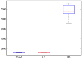
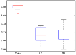
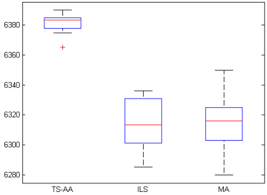
5.2 Distribution of the best objective function values

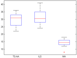
In addition to the Borda aggregation method presented above, the boxplots shown in figures 5-8 illustrate the magnitude and distribution of the best objective values (at the end of the run) for a selected instance of each domain. Each figure represents the result of 10 runs from each algorithm. Arbitrarily we selected instance number 1 from each domain, but similar distributions of results can be observed in the other instances.

From figures 5-8, it can be observed that the performance of the three algorithms differs significantly over the four problem instances. For example, in the max-sat instance (figure 5) the memetic algorithm (MA) performs the best, while it performs the worst in personnel scheduling instance(figure 8). The tabu search hyper-heuristic (TS-AA) clearly performs the worst on the instances of bin packing and flow shop (Figures 6-7), but performs the best on the personnel scheduling instance. The scale of Figure 8 means that it is difficult to see the difference between TS-AA and ILS. This is because the personnel scheduling domain applies penalties to solution that violates the constraints, and the memetic algorithm produced poor solutions in this instance.

In summary, these boxplots show that it is challenging to design an algorithm which operates well over all the problem domains. When an algorithm improves on one domain, its solution quality may reduce on another domain. This can also be true in a single domain, when an algorithm improves on a particular problem instance, and its performance reduces on other instances of that domain. The challenge is to design online learning mechanisms that can adapt on the fly, and thus select the most adequate heuristic at each decision step, using the feedback gathered from the search process.

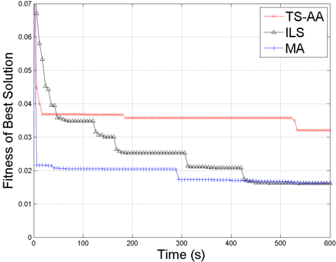
5.3 Progress of algorithms during a run

Figure 9 shows the progress of the three algorithms during one 10 minute run on instance 1 of Bin Packing. A lower fitness value represents a better solution. This information is easily available from within HyFlex by calling the getFitnessTrace()

method, and it is automatically recorded during the run. They show that the performance of the algorithms can differ greatly depending on how long they are left to run. Iterated local search (ILS) and the memetic algorithm (MA) both finish the run at approximately the same fitness. However, the memetic algorithm finds better quality solutions more quickly. The tabu search hyper-heuristic (TS-AA) begins the run by finding better solutions than ILS, but TS-AA stagnates, and by the end of the run ILS has found a better solution. This ability to easily obtain useful information for analysis is another way that HyFlex can save a significant amount of time for researchers.

6 Conclusions

This paper has presented and described the HyFlex software framework for the development of cross-domain heuristic search methodologies. HyFlex provides multiple problem domains, each containing a set of problem instances and search operators to apply. Therefore, it represents a novel extension of the notion of benchmark for combinatorial optimisation, with which cross-domain algorithms can be easily developed, and reliably compared. Researchers from different communities and themes within computer science, artificial intelligence and operational research, can potentially benefit from HyFlex, as it provides a common benchmark in which to test the performance and behavior of single-point and population-based self-configuring search heuristics. When using HyFlex, researchers can concentrate their efforts on designing their adaptive methodologies, rather than implementing the required set of problem domains.

This paper describes the architecture of HyFlex, including examples of how to create and run hyper-heuristics within the framework. The four problem domains are presented and discussed, and three example hyper-heuristics are analysed, with their results. The results show that the hyper-heuristics all have differing performances on the

four problem domains. No one algorithm is superior to the other two algorithms on all four problem domains. Although these are not state-of-the-art adaptive algorithms, the results suggest that there is still considerable scope for future research when desiging adaptive and self-configuring algorithms that can learn from the search process and select the most suitable search operators.

There is currently ample evidence that HyFlex is useful to the research community, due to the number of researchers which are currently employing it for their research and teaching. The HyFlex framework was made publicly available in August 2010. In May 2011, the software had been downloaded over 460 times, and the associated web-pages describing it had been visited over 11,844 times. The community has also responded well to a call for participation in the International Cross-domain Heuristic Search Challenge (CHeSC), which would not be possible without the HyFlex software. In May 2011, the competition had 43 registered participants and teams from 23 different countries.

HyFlex can be extended to include new domains, additional instances and operators in existing domains, and multi-objective and dynamic problems. The current software interface can also be extended to incorporate additional feedback information from the domains to guide the adaptive search controllers. It is our vision that the HyFlex framework will continue to facilitate and increase international interest in developing adaptive heuristic search methodologies, that can find wider application in practice.

References

• Argelich J, Li CM, Manya F, Planes J (2009) Maxsat evaluation 2009 benchmark data sets. Website, http://www.maxsat.udl.cat/
• Bai R, Blazewicz J, Burke EK, Kendall G, McCollum B (2007) A simulated annealing hyperheuristic methodology for flexible decision support. Tech. rep., University of Nottingham
• Battiti R (1996) Reactive search: Toward self-tuning heuristics. In: Rayward-Smith VJ, Osman IH, Reeves CR, Smith GD (eds) Modern Heuristic Search Methods, John Wiley & Sons Ltd., Chichester, pp 61-83
• Battiti R, Brunato M, Mascia F (2009) Reactive Search and Intelligent Optimization, Operations Research/Computer Science Interfaces Series, vol 45. Springer
• Baxter J (1981) Local optima avoidance in depot location. Journal of the Operational Research Society 32:815-819
• Beasley JE (2010) Or-library: collection of test data sets for a variety of operations research (or) problems. Website, http://people.brunel.ac.uk/ ~ mastjjb/jeb/info.htmll
• Bierwirth C, Mattfeld DC, Kopfer H (1996) On permutation representations for scheduling problems. In: Voigt H, Ebeling W, Rechenberg I, Schwefel H (eds) LNCS 1141: Proceedings of the 4th Parallel Problem Solving from Nature Conference (PPSN'96), Berlin, Germany, pp 310-318
• Blanton JL Jr, Wainwright RL (1993) Multiple vehicle routing with time and capacity constraints using genetic algorithms. In: Proceedings of the 5th International Conference on Genetic Algorithms, Morgan Kaufmann Publishers Inc., San Francisco, CA, USA, pp 452459, URL http://portal.acm.org/citation.cfm?id=645513.657758
• Bleuler S, Laumanns M, Thiele L, Zitzler E (2003) PISA-A Platform and Programming Language Independent Interface for Search Algorithms. In: Conference on Evolutionary Multi-Criterion Optimization (EMO 2003), Springer, Berlin, LNCS, vol 2632, pp 494-508
• Braysy O (2002) A reactive variable neighborhood search for the vehicle-routing problem with time windows. INFORMS Journal on Computing 15(4):347-368
• Burke EK, Cowling P, De Causmaecker P, Vanden Berghe G (2001) A memetic approach to the nurse rostering problem. Applied Intelligence 15(3):199-214
• Burke EK, Hart E, Kendall G, Newall J, Ross P, Schulenburg S (2003a) Hyper-heuristics: An emerging direction in modern search technology. In: Glover F, Kochenberger G (eds) Handbook of Metaheuristics, Kluwer, pp 457-474

• Burke EK, Kendall G, Soubeiga E (2003b) A tabu-search hyper-heuristic for timetabling and rostering. Journal of Heuristics 9(6):451-470
• Burke EK, Curtois T, Qu R, Vanden Berge G (2007) A time predefined variable depth search for nurse rostering. Tech. rep., School of Computer Science, University of Nottingham
• Burke EK, Curtois T, Post G, Qu R, Veltman B (2008) A hybrid heuristic ordering and variable neighbourhood search for the nurse rostering problem. European Journal of Operational Research 188(2):330-341
• Burke EK, Curtois T, Hyde M, Kendall G, Ochoa G, Petrovic S, Vazquez-Rodriguez JA, Gendreau M (2010a) Iterated local search vs. hyper-heuristics: Towards general-purpose search algorithms. In: IEEE Congress on Evolutionary Computation (CEC 2010), Barcelona, Spain, pp 3073-3080
• Burke EK, Curtois T, Qu R, Vanden Berge G (2010b) A scatter search methodology for the nurse rostering problem. Journal of the Operational Research Society 61:1667-1679
• Burke EK, Hyde M, Kendall G, Ochoa G, Ozcan E, Woodward J (2010c) Handbook of Metaheuristics, International Series in Operations Research & Management Science, vol 146, Springer, chap A Classification of Hyper-heuristic Approaches, pp 449-468. DOI DOI:10.1007/978-1-4419-1665-5, chapter 15
• CHeSC (2011) The First Cross-domain Heuristic Search Challenge, CHeSC 2011. Website, http://www.asap.cs.nott.ac.uk/chesc2011/
• Cowling P, Kendall G, Soubeiga E (2000) A hyperheuristic approach to scheduling a sales summit. In: Burke EK, Erben W (eds) Proceedings of the 3rd International Conference on the Practice and Theory of Automated Timetabling (PATAT 2000), Konstanz, Germany, pp 176-190
• CRIL (2007) Sat competition 2007 benchmark data sets. Centre de Recherche en Informatique de Lens, Website, http://www.cril.univ-artois.fr/SAT07/
• CRIL (2009) Sat competition 2009 benchmark data sets. Centre de Recherche en Informatique de Lens, Website, http://www.cril.univ-artois.fr/SAT09/
• Curtois T (2009) Staff rostering benchmark data sets. Website, http:///www.cs.nott.ac.uk/ ~ tec/NRP/
• Curtois T (2010) A hyflex module for the personnel scheduling problem. Tech. rep., School of Computer Science, University of Nottingham
• Davis L (1985) Job shop scheduling with genetic algorithms. In: Grefenstette JJ (ed) Proceedings of the 1st International Conference on Genetic Algorithms and their Applications, Hillsdale, NJ, USA, pp 136-140
• Eiben AE, Michalewicz Z, Schoenauer M, Smith JE (2007) Parameter Setting in Evolutionary Algorithms, Springer, chap Parameter Control in Evolutionary Algorithms, pp 19-46
• ESICUP (2011) European special interest group on cutting and packing benchmark data sets. Website, http://paginas.fe.up.pt/ ~ esicup/
• Fialho A, Costa LD, Schoenauer M, Sebag M (2008) Extreme value based adaptive operator selection. In: Parallel Problem Solving from Nature PPSN X, Lecture Notes in Computer Science, vol 5199, Springer Berlin / Heidelberg, pp 175-184
• Fialho A, Da Costa L, Schoenauer M, Sebag M (2010) Analyzing bandit-based adaptive operator selection mechanisms. Annals of Mathematics and Artificial Intelligence - Special Issue on Learning and Intelligent Optimization DOI 10.1007/s10472-010-9213-y
• Fukunaga AS (2008) Automated discovery of local search heuristics for satisfiability testing. Evolutionary Computation (MIT Press) 16(1):31-1
• Gent I, Walsh T (1993) Towards an understanding of hill-climbing procedures for sat. In: Proceedings of the 11th National Conference on Artificial Intelligence (AAAI'93), Washington D.C., USA, pp 28-33
• Goldberg DE, Lingle R (1985) Alleles, loci, and the traveling salesman problem. In: Grefenstette JJ (ed) Proceedings of the 1st International Conference on Genetic Algorithms and their Applications, Hillsdale, NJ, USA, pp 154-159
• Hyde MR (2011) One dimensional packing benchmark data sets. Website, http://www.cs. nott.ac.uk/ ~ mvh/packingresources.shtml
• Ikegami A, Niwa A (2003) A subproblem-centric model and approach to the nurse scheduling problem. Mathematical Programming 97(3):517-541
• Jakob W (2006) Towards an adaptive multimeme algorithm for parameter optimisation suiting the engineers' needs. In: Parallel Problem Solving from Nature - PPSN IX, 9th International Conference, Reykjavik, Iceland, September 9-13, 2006, Procedings, Springer, Lecture Notes in Computer Science, vol 4193, pp 132-141

• Johnson D, Demers A, Ullman J, Garey M, Graham R (1974) Worst-case performance bounds for simple one-dimensional packaging algorithms. SIAM Journal on Computing 3(4):299-325
• Krasnogor N, Smith JE (2001) Emergence of profitable search strategies based on a simple inheritance mechanism. In: Proceedings of the 2001 Genetic and Evolutionary Computation Conference, Morgan Kaufmann
• Lobo FG, Lima CF, Michalewicz Z (eds) (2007) Parameter Setting in Evolutionary Algorithms, Studies in Computational Intelligence, vol 54. Springer
• Lourenco HR, Martin O, Stutzle T (2002) Iterated Local Search, Kluwer Academic Publishers,, Norwell, MA, pp 321-353
• Martello S, Toth P (1990) Knapsack Problems: Algorithms and Computer Implementations. John Wiley and Sons, Chichester
• Martin O, Otto SW, Felten EW (1992) Large-step Markov chains for the TSP incorporating local search heuristics. Operations Research Letters 11(4):219-224
• Maturana J, Saubion F (2008) A compass to guide genetic algorithms. In: Proceedings of the 10th international conference on Parallel Problem Solving from Nature, Springer-Verlag, Berlin, Heidelberg, pp 256-265
• Maturana J, Lardeux F, Saubion F (2010) Autonomous operator management for evolutionary algorithms. Journal of Heuristics 16(6):1881-909
• McAllester D, Selman B, Kautz H (1997) Evidence for invariants in local search. In: Proceedings of the 14th National Conference on Artificial Intelligence (AAAI), Providence, Rhode Island, USA, pp 459-465
• Mladenovic N, Hansen P (1997) Variable neighborhood search. Computers and Operations Research 24(11):1097-1100
• Nawaz M, Jr EE, Ham I (1983) A heuristic algorithm for the m -machine, n -job flow-shop sequencing problem. OMEGA-International Journal of Management Science 11(1):91-95
• Neri F, Toivanen J, Cascella GL, Ong YS (2007) An adaptive multimeme algorithm for designing HIV multidrug therapies. IEEE/ACM Trans Comput Biology Bioinform 4(2):264-278
• Ong YS, Lim MH, Zhu N, Wong KW (2006) Classification of adaptive memetic algorithms: a comparative study. IEEE Transactions on Systems, Man, and Cybernetics, Part B 36(1):141152
• Pisinger D, Ropke S (2007) A general heuristic for vehicle routing problems. Computers and Operations Research 34:2403- 2435
• Rohlfshagen P, Bullinaria J (2007) A genetic algorithm with exon shuffling crossover for hard bin packing problems. In: Proceedings of the 9th annual conference on Genetic and evolutionary computation (GECCO'07), London, U.K., pp 1365-1371
• Ross P (2005) Hyper-heuristics. In: Burke EK, Kendall G (eds) Search Methodologies: Introductory Tutorials in Optimization and Decision Support Techniques, Springer, chap 17, pp 529-556
• Ruiz R, St¨ utzle TG (2007a) An iterated greedy heuristic for the sequence dependent setup times flowshop problem with makespan and weighted tardiness objectives. European Journal of Operational Research 187(10):1143-1159
• Ruiz R, St¨ utzle TG (2007b) A simple and effective iterated greedy algorithm for the permutation flowshop scheduling problem. European Journal of Operational Research 177:2033-2049
• Selman B, Levesque H, Mitchell D (1992) A new method for solving hard satisfiability problems. In: Proceedings of the 10th National Conference on Artificial Intelligence (AAAI'92), San Jose, CA, USA, pp 440-446
• Selman B, Kautz H, , Cohen B (1994) Noise strategies for improving local search. In: Proceedings of the 11th National Conference on Artificial Intelligence (AAAI'94), Seattle, WA, USA, pp 337-343
• Smith JE (2007) Co-evolving memetic algorithms: A review and progress report. IEEE Transactions in Systems, Man and Cybernetics, part B 37(1):6-17
• Taillard E (1993) Benchmarks for basic scheduling problems. European Journal of Operational Research 64(2):278-285
• Taillard E (2010) Flow shop benchmark data sets. Website, http://mistic.heig-vd.ch/ taillard/
• Talbi EG (2009) Metaheuristics: from design to implementation. Wiley
• TSPLIB (2008) Tsplib: a library of sample instances for the tsp (and related problems). Website, http://www.iwr.uni-heidelberg.de/iwr/comopt/soft/TSPLIB95/TSPLIB.html