Implementation of Continuous Bayesian Networks Using Sums of Weighted Gaussians

Eric Driver and Darryl Morrell Telecommunications Research Center and Department of Electrical Engineering Arizona State University Tempe, AZ 85287

Abstract

Bayesian networks provide a method of rep­ resenting conditional independence between random variables and computing the prob­ ability distributions associated with these random variables. In this paper, we ex­ tend Bayesian network structures to compute probability density functions for continuous random variables. We make this extension by approximating prior and conditional den­ sities using sums of weighted Gaussian dis­ tributions and then finding the propagation rules for updating the densities in terms of these weights. We present a simple exam­ ple that illustrates the Bayesian network for continuous variables; this example shows the effect of the network structure and approxi­ mation errors on the computation of densities for variables in the network.

1 INTRODUCTION

Bayesian networks provide a method of represent­ ing conditional independence relationships between random variables and of computing the probabil­ ity distributions associated with these random vari­ ables. Bayesian networks were originally developed for discrete-valued random variables; there is an increas­ ing interest in extending this approach to continuous­ valued random variables. Previous work on networks of continuous-valued variables has required that the variables have Gaussian density functions and that the relationships between these variables be linear(Pearl 1988, Shachter 1989). Theoretical issues involving the representation of relationships between random vari­ ables using a network (directed or undirected graph) consisting of both continuous and discrete random variables, including tests for conditional independence, are addressed in (Lauritzen 1989, Lauritzen 1990); an approach to updating conditional probabilities in which a single Gaussian is used to approximate a mix­ ture of Gaussian densities is given in (Spiegelhalter 1990). In this paper, we extend Bayesian networks

to include random variables with arbitrary distribu­ tions. We make this extension by approximating prior and conditional densities using sums of weighted Gaus­ sian distributions; to our knowledge, this is the first time this approximation technique has been used in Bayesian networks. Using this technique, we find prop­ agation rules for updating the densities of the network variables; information propagates through the network in the form of messages consisting of weight, mean, and variance updates.

2 PRELIMINARIES

We implement Bayesian networks for continuous vari­ ables by approximating both prior and conditional density functions by sums of weighted Gaussian den­ sities. A density so approximated is represented in terms of a set of weights, a set of means, and a set of variances. Computation of these approximations is a hard problem which we discuss in Section 5.

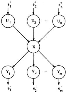
Figure 1 shows a fragment of a Bayesian network. For our implementation, we assume that the network is singly connected (i.e. at most one path connects any two variables) and we assume that X is related to its

parent nodes U1, U 2 , · · · , Un by

where g is an arbitrary function and Wx is a noise term assumed to be Gaussian with zero mean and uncorre­ lated with any other noise term or node in the network. In section 3. 5 we consider the case when g is linear.

From ( 1 ) , we have:

where N(x;u 2 ,J.L) is the Gaussian distribution defined by:

We approximate f(xJu1, . . . , un) by a weighted sum of Gaussians as follows:

where M is the number of Gaussians used to approxi­ mate f (xJut, . . . , un). Note that the approximation in ( 4) is capable of representing conditional density func­ tions that do not embody the relationship between X and U1, U 2 , . . . , Un given in ( 1 ) ; thus, this approach can be used in more general settings than considered here. Again, we refer to Section 5 for a discussion of how the weights { C j }, means { f-L�j} , and variances { uJ} can be determined to approximate a given con­ ditional density function.

Using this approximation, we show that all belief func­ tions and messages can be represented as sums of weighted Gaussians. Before proceeding, we state with­ out proof the following identity which will be useful in the upcoming derivations:

where a = N(J.Ll; u1 2 + u2 2 , f..L 2) is a constant with re­ spect to x.

3 THE PROPAGATION RULES

We first consider an arbitrary node X shown in Fig­ ure 1. The parents of X are U1, U 2 , . . . , Un and the children of X are Y1, Y 2 , . .. , Ym. We assume to begin that X has not been instantiated. The case when X has been instantiated and also the case when X has no parents or no children is considered in Section 3. 4.

3.1 COMPUTATION OF BEL(X)

Let e1 denote the evidence in the subnetwork above X and let ex denote the evidence in the subnet­ work below X. Also, let et (i = 1,2, . . . ,n ) de­ note the evidence coming to X via node U;, and let ej(j = 1,2, . . . ,m ) denote the evidence coming to X via node }j. We assume X has received messages 7rx(u;)(i = 1,2, .. . ,n ) from its parents; each message is a sum of weighted Gaussians:

where M; is the number of Gaussian densities in the representation for 1r x ( u;), { aL } is a set of real valued weights, { (u�.k,r} is a set of real valued variances, and {f-L�, k ;} is a set of real valued means. Sim­ ilarly, we assume X has received messages Ay;(x)(j = 1, 2, .. . , m) from its children:

where Pi is the number of Gaussian densities in the representation for Ay; ( x), {,ef;} is a set of real valued weights, { ( a{,l;) 2 } is a set of real valued variances, and {f-L{. I ;} is a set of real valued means.

The belief function for X is computed as follows:

where a = f(e)(lle f ) is a normalization constant.

We compute 1r( x) as follows:

where we have defined:

We now compute A(x), but first we make some def­ initions. Let C denote the set of child nodes of X, let R = {j E Clej -::J 0} , and let r be the number of elements in R. Next, we relabel the child nodes so that nodes Y1 through Yr correspond to the nodes with ej =j:. 0 . If r = 0 then A(x) � f 1. If r = 1 then A(x) � f Ayr(x). For r 2:: 2, we compute A(x) as follows:

Using the fact that a product of Gaussians is propor­ tional to a Gaussian we can see that (11) is indeed a weighted sum of Gaussians. We refer the reader to (Driver 1995) for a complete derivation. We write A(x) in the following form:

where Mo = IJ� = l Pi, { aio } is a set of real valued weights, {(17>. ,j0 ) 2} is a set of real valued variances, and {J-t io } is a set of real valued means.

We can now compute BEL(x) by forming the product of (12) and (9). BEL(x) can then be written as a weighted sum of Gaussians by using (5):

where

and a is a normalization constant chosen so that J BEL(x)dx = 1. Integrating (13) with respect to x, it follows that

3.2 TOP DOWN PROPAGATION

The message 1ry1(x) that node X sends to its jth child (j = 1, 2, .. . , m ) is formed as follows:

So 1ry1 ( x) can be computed by the method of the last section with the assumption that AyAx) = 1.

3.3 BOTTOM UP PROPAGATION

The message Ax ( u;) that node X sends to its ith par­ ent ( i = 1, 2, ... , n ) is formed as follows:

Consider the first distribution in the integrand:

Where C = f1�=1 f( et) is constant for a given set of kf;i evidence. Next, consider the second distribution in the integrand:

Substituting (18) and (19) into (17), we have:

The constant C will get absorbed during the normalization of BEL(x), so we can ignore it. J(xiu1, . .. ,un), A(x), and 7rx(uk) are given by ( 4 ) , ( 12 ), and (6) respectively. Substituting these into ( 20 ) we have:

where we have defined:

Note that if A(x) is constant then from ( 20 ) we have:

Hence, if A(x) = 1 then Ax(u;) = 1 for each i. So just like with discrete variables, evidence gathered at a node does not affect any spousal nodes until their common child node obtains evidence.

3.4 BOUNDARY CONDITIONS

If X is a root node (i.e. a node with no parents) that has not been instantiated, then we set 1r( x) equal to the prior density function f( x). This prior distribution is approximated by a sum of weighted Gaussians.

If X is a leaf node (i.e. a node with no children) that has not been instantiated, then we set A( x) = 1. This implies that BEL(x) = 1r(x).

If X is an evidence node, say X = x0, then we set A(x) = c5(x- x0) = N(x; 0, xo) regardless of the in­ coming A-messages. This implies that BEL(x) = N(x; 0, x0) as we would expect. Furthermore, for each j, 1Tyi(x) = N(x; 0, xo) is the message that node X sends to its children (each child gets the same message in this case). The messages that node X sends to its parents are still weighted sums of Gaussians.

3.5 SPECIAL CASE: LINEARITY

In this section, we consider the special case when the function g of Equation ( 1) has the form

where the b; 's are real numbers. This relationship was suggested in (Pearl 1988). With this we have

We note that only the computations of 1r( x) and Ax(u;) involve the distribution f(xJul, . . . , un), so all other computations are the same as before. Further­ more, we can obtain closed form solutions for 1r( x) and Ax ( u;) without invoking the approximation given by (4). To do so, we use the following identity:

For completeness we state the final result but omit the proof; we refer the interested reader to (Driver 1995):

Note that the means and variances of the Normal dis­ tributions in (26) and (27) have the same form as those in Pearl's result. The only real difference here is that our result is a sum of weighted Gaussians and Pearl's result is a single Gaussian.

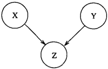
4 EXAMPLE

In this section, we present a simple example that illus­ trates the characteristics of this approach to continu­ ous Bayesian networks. The example uses the network of Figure 2. Nodes X andY are independent and uni­ formly distributed on [0, 1]. Node Z is related to X and Y by the following equation:

where wz is a Gaussian random variable with zero mean and variance 0.01 ; wz is independent of X and Y.

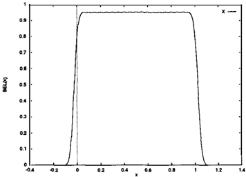
Figure 3 shows a graph of our approximation to the prior distributions of nodes X and Y; this approxima­ tion consists of 20 Gaussians with uniformly spaced

means, equal variances, and equal weights. The abso­ lute error in this approximation is 9%. Other approxi­ mations could be found that provide a better represen­ tation of the densities with fewer Gaussians; potential methods by which this can be done are discussed in Section 5.

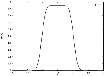
Performing the updating algorithm with no evidence in the network, we obtain the distribution for node Z. This is shown in Figure 4. From probability theory, we know that the distribution of a sum of two independent random varibles is the convolution of the individual distributions. So theoretically, the distribution of Z should be the triangular function on the interval [ 0 , 2 ]. Taking into account the effects of the noise wz and the approximation error in the prior distributions, this is exactly what we have in Figure 4.

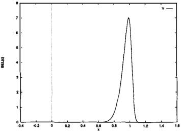
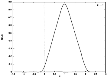
Next, we assume that node X is instantiated at a value of 1.0. Performing the updating algorithm for this evidence, we obtain the belief function for node Z. This is shown in Figure 5. We can explain this as follows. Given X = 1.0, Z is just the sum of the constant 1.0 and a uniform distribution (plus the noise term wz ) . Hence, Z is a uniform distribution on [ 1 , 2]. This is approximately what we have in Figure 5. Node Y of course remains unchanged since it is independent of X.

Now we reinitialize the network and assume we have

observed node Z = 2.0. Performing the updating algo­ rithm for this evidence, we obtain the belief function for node X. This is shown in Figure 6. The only way that Z can equal 2.0 is if both X andY are 1.0, so the distributions for X and Y should be delta functions centered at 1.0. From Figure 6, we see that our results are a reasonable approximation to a delta function, es­ pecially when we consider the effects of the noise and the approximation error in the prior density functions.

5 GAUSSIAN SUM APPROXIMATIONS

In this section, we discuss briefly some of the issues involved in choosing sum-of-Gaussian approximations to probability density functions. We first discuss the existence of good approximations. We then mention several techniques that can be used to obtain these approximations.

LetS be a compact subset ofnn and consider the set:

where C[S] is the set of all continuous functions from S ton. By a simple application of the Stone-Weierstrass theorem, it can be shown (Girosi 1990) that gs is dense in C[S]. That is, given any f E C[S] and any c > 0, there exists g E gs such that f s Jg(x) - f(x)JdV < t. (Note: here we have used the L1 norm, in fact the result holds for any Lp norm, 1 � p < oo. ) In other words, any arbitrary function in C[S] can be approx­ imated arbitrarily well by a finite sum of weighted Gaussians.

In this paper, the functions we are approximating are probability density functions. Since density functions die off at infinity, as an approximation we may assume that they are defined on compact subsets of nn ( i.e. we set them to zero outside some compact subset of nn). Hence, by the above results it is reasonable to assume that any density function can be approximated arbitrarily well by a finite sum of Gaussians.

We now turn our attention to actually finding such approximations. One approach to obtaining approxi­ mations is the use of neural networks (Poggio 1990). Another method (Klopfenstein 1983) approximates an arbitrary function by uniformly spaced Gaussians; us­ ing Fourier transform techniques, error estimates can be obtained. Other methods include simmulated an­ nealing and gradient descent algorithms. Our best re­ sults have been with the gradient descent algorithm, especially when approximating functions with a small number of variables.

Acknowledgements

This work supported by the United States Army Re­ search Office, grant number DAAH04-93-G-0218

References

1. Pearl, Probabilistic Reasoning In Intelligent Sys­ tems. San Mateo, CA: Morgan Kaufmann Publishers, 1988.
2. D. Shachter and C. R. Kenley, "Gaussian Influence Diagrams," Management Science, Vol. 35, No.5, May 1989, pp. 527-550.
3. L. Lauritzen and N. Wermuth, "Graphical Models for Associations Between Variables, Some of Which are Qualitative and Some Quantitative," The Annals of Statistics, Vol. 17, No. 1, 1989, pp. 31-57.
4. L. Lauritzen, A. P. Dawid, B. N. Larsen, and H. G. Leimer, "Independence Properties of Directed Markov Fields," Networks, Vol. 20, Iss. 5, Aug 1990, pp. 491-505.
5. J. Spiegelhalter and S. L. Lauritzen, "Sequen­ tial Updating of Conditional Probabilities on Directed Graphical Structures," Networks, Vol. 20, Iss. 5, Aug 1990, pp. 579-605.
6. Driver and D. Morrell, "Implementation of Continu­ ous Bayesian Networks Using Sums of Weighted Gaus-
7. sians," Technical Report TRC-SP-DRM-9501, Electri­ cal Engineering Department, ASU, May 1995.
8. Girosi and T. Poggio, "Networks and the Best Approximaton Property," Biological Cybernetics, Vol. 63, 1990, pp. 169-176.
9. Poggio and F. Girosi, "Networks for Approxima­ tion and Learning," Proceedings o f the IEEE, Vol. 78, No. 9, Sep. 1990,pp. 1481-1497.
10. Klopfenstein and R. Sverdlove, "Approximation by Uniformly Spaced Gaussian Functions," in Approxi­ mation Theory IV, (C. K. Chui, L. L. Schumaker, and J.D. Ward, eds.), pp. 575-580, Academic Press, 1983.