Incremental computation of the value of perfect information in stepwise-decomposable influence diagrams

(Nevin) Lianwen Zhang, Runping Qi, and David Poole

Department of Computer Science University of British Columbia Vancouver, B.C., Canada { !zhang, qi, poole } @cs. ubc.ca

Abstract

To determine the value of perfect informa­ tion in an influence diagram, one needs first to modify the diagram to reflect the change in information availability, and then to com­ pute the optimal expected values of both the original diagram and the modified diagram. The value of perfect information is the dif­ ference between the two optimal expected values. This paper is about how to speed up the computation of the optimal expected value of the modified diagram by making use of the intermediate computation results ob­ tained when computing the optimal expected value of the original diagram.

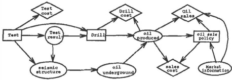
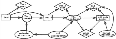
drill. This means that the drill decision is to be made knowing the type of test per­ formed and the test-result. There is no arc from market-information to drill. This means that market-information ( at the time when the oil-sale-policy is to be made ) is not available at the time the drill decision is to be made.

1 INTRODUCTION

The concept of the value of perfect information is very useful in gaining insights about decision problems. Matheson (1990) has demonstrated that influence di­ agrams provide a more suitable paradigm to address the issue than decision trees. This paper is concerned with the problem of computing the value of perfect information in influence diagrams.

An influence diagram is a graphical representation of a particular decision problem ( Howard and Matheson 1984). It is an acyclic directed graph with three types of nodes: decision nodes, random nodes and value nodes. The influence diagram in Fig. 1 represents an extension to the well-known oil wildcatter problem ( Raiffa 1968, Shachter 1986). The decision nodes are depicted as rectangles, random nodes as ellipses, and value nodes as diamonds.

The total value of the diagram is oil-sales minus the sum of test-cost, drill-cost, and sale-cost. The expectation of the total value depends on the decisions made. The optimal expected value of the diagram is de­ fined to be the maximum of the expected total values.

There are arcs from test and test-result to

To reduce risks, the oil wildcatter may choose to, before making the drill decision, hire an expert to predicate market-information at the time the oil-sale-policy is to be made. This operation may be expensive. So, before making up his mind, the oil wildcatter may wish to determine the value of the ex­ pert's predications. The value of perfect information on market-information serves as an upper bound for the value of the predications. Specifically, it is defined as follows. Modify the diagram by adding an arc from market-information to drill. The value of perfect information on market-information is the difference between the optimal expected value of the modified diagram and that of the original diagram.

A straightforward method of computing the value of perfect information is to exactly follow the definition. That is to respectively compute the optimal expected values of the original influence diagram and of the modified diagram, and then figure out the difference. This paper shows that one can do better than that. Since the original and the modified diagrams differ very little, there must be computation overlaps in the processes of evaluating them. By avoiding those over­ laps, one can speed up computing the optimal ex-

pected value of the modified diagram. This is espe­ cially interesting if one wants to assess the value of perfect information for a number of cases.

The exposition will be carried out in the terms of stepwise-decomposable influence diagrams, which is reviewed in section 2. Section 3 introduces the concept of influence diagram condensation. Section 4 shows how to use this concept to uncover the computation overlaps mentioned in the previous paragraph. The paper concludes at section 5.

2 STEPWISE-DECOMPOSABLE INFLUENCE DIAGRAMS

Stepwise-decomposable influence diagrams (SDID's) were first introduced by Zhang and Poole (1992) as a generalization to the traditional notion of influence diagrams. Better references in this regard are Zhang, Qi and Poole (1993b) and Zhang (1993). This section reviews the concept of SDID's.

2.1 THE PATH TO SDID'S

Traditionally, there are five constraints imposed on in­ fluence diagrams:

1. Acyclicity, which requires that there be no di­ rected loops in influence diagrams;
2. Regularity, which requires that there be a total ordering among all the decision nodes;
3. The no-forgetting constraint, which requires that any decision node and its parents be parents to all subsequent decision nodes;
4. The single-value-node constraint, which requires that there be only one value node; and
5. The leaf-value-node constraint, which requires that the value node have no children.

Influence diagrams that satisfy all the five constraints will be referred to as no-forgetting influence diagrams.

We propose to lift constraints 2-4 and to develop a general theory of influence diagrams starting with con­ straints 1 and 5 only.

There are several advantages to lift constraints 2-4. For instance, by lifting the no-forgetting constraint we are able to, anmong other things, represent the facts that some decision nodes are conditionally indepen­ dent of certain pieces of information. In the extended oil wildcatter problem (Fig. 1), it is reasonable to as­ sume that the decision oil-sale-policy is indepen­ dent of information on test-result given the quality and quantity of oil-produced. This piece of knowl­ edge can not be represented if the no-forgetting con­ straint is enforced. The reader is referred to Zhang (1993), Zhang, Qi and Poole (1993) for other rationale for lifting constraints 2-4.

Note: Traditionally, arcs into decision nodes are inter­ preted as indications of information availability. Now that the no-forgetting constraint has been lifted, those arcs need to be re-interpreted as indication of both information availability and dependency. More explic­ itly, the lack of an arc from a node c to a decision node d no longer implies that information c is not observed when making decision d. It may as well mean that d is independent of c given the parents of d.

Acyclicity and the leaf-node constraint together de­ fine a very general concept of influence diagrams. One theme of Zhang (1993) is to identify subclasses of in­ fluence diagrams with various computational proper­ ties. One important property for an influence diagram to possess is the so-called stepwise-solvability, which says that the diagram can be evaluated by considering one decision node at a time. If an influence diagram is not stepwise-solvable, then one needs to simulta­ neously consider several, even all the decision nodes, which usually tends to be computationally expensive.

When an influence diagram is stepwise-solvable? The answer: when it is stepwise-decomposable. It can be shown that a stepwise-decomposable influence di­ agram can be evaluated not only by considering one decision node at a time, but also by considering one section of the diagram at a time (Zhang, Qi and Poole 1993). It can also be shown that an influence di­ agram is stepwise-solvable only when it is stepwise­ decomposable (Zhang 1993).

In the rest of this section, we define stepwise­ decomposable influence diagrams.

2.2 INFLUENCE DIAGRAMS

An influence diagram is an acyclic directed graph con­ sisting of a set of random nodes C, a set of decision nodes D, and a set of value nodes U. The value nodes have no children. A random node c represents an un­ certain quantity whose value is determined according to a given conditional probability distribution P(cJ7rc), where 7r c stands for the set of the parents of c. A value node v represent one portion of the decision maker's utilities, which is characterized by a value function f v.

Let I be an influence diagram. For any node x in I, let 'lrx denote the set of the parents of X . Let nx denote the frame of x, i.e the set of possible values of x. For any set J of nodes, let nJ = nxEJ nx.

Let d1, ... , dk be all the decision nodes in I. For a decision node d;, a mapping 8; : n.,.d· ---+ nd, is called a decision function for d;. The set � f all the decision functions for d;, denoted by di, is called the decision function space for d;. The Cartesian product of the decision function spaces for all the decision nodes is called the policy space of I. We denote it by .6..

Given a policy 8 = (81, ... , 8k) E .6. for I, a probabil­ ity P0 can be defined over the random nodes and the

decision nodes as follows:

where P(cl7rc) is given in the specification of the influ­ ence diagram, while P6;(dil11"d;) is given by Oi as fol­ lows:

For any value node v, 11"11 must consist of only deci­ sion and value nodes, since value nodes do not have children. Hence, we can talk about P0(7r11). The ex­ pectation of the value node v under Po, denoted by E5[v], is defined as follows:

The summation of the expectations of all the value nodes is called the value of I under the policy 6, We denote this denoted by E5[I]. The maximum of E5[I) over all the possible policies 6 is the optimal expected value of I. An optimal policy is a policy that achieves the optimal expected value. To evaluate an influence diagram is to determine its optimal expected value and to find an optimal policy.

An influence is regular if there exists a total ordering among all the decision nodes. Even though all our results in this paper readily generalizes to influence diagrams which are not necessarily regular, we shall limit the exposition only to regular influence diagrams for the sake of simplicity.

2.3 STEPWISE-DECOMPOSABLE INFLUENCE DIAGRAMS

To introduce stepwise-decomposable influence dia­ grams (SDID), we need the concepts of moral graph and of m-separation. Let G be a directed graph. The moral graph G is an undirected graph m( G) with the same vertex set as G such that there is an edge be­ tween two vertices in m ( G) if and only if either there is an arc between them in G or they share a common child in G. The term moral graph was chosen because two nodes with a common child are "married" into an edge (Lauritzen and Spiegehalter 1988).

In an undirected graph, two nodes x and y are sepa­ rated by a set of nodes A if every path connecting them contains at least one node in A. In a directed graph G, x and y are m-separated by A if they are separated by A in the moral graph m( G). One implication of this definition is that A m-separates every node in A from any node outside A.

For any decision node d of I, the downstream of 7r d is the set of nodes that are not m-separated from d by 7r d. The upstream of 7r d is that set of nodes outside 7r d that are m-separated from d by 7rd.

A regular influence diagram is stepwise-decomposable if for any decision node d, none of the decision nodes that precede d are in the downstream of 71" d.

The influence diagram in Fig. 1 is a SDID. No­ forgetting influence diagrams are SDID's.

One desirable property of SDID's is that they are stepwise-solvable. As an example, consider the SDID in Fig. 1. One can first compute an optimal policy for oil-sale-policy in the part of the diagram that lies to the right of oil-produced with oil-produced included, and then find an optimal policy for drill, and then for test. The optimal expected value of the diagram obtained as a by-product of computing an optimal policy for test. See Zhang, Qi and Poole (1993b) for details.

3 CONDENSING SDID'S

This section presents a two-stage approach for evaluat­ ing SDID's. In the first stage, a SDID is "condensed" into a Markov decision process (Denardo 1982). This involves two types of operations: the operation of com­ puting conditional probabilities and the operation of summing up several functions. In the second stage, the condensed SDID is evaluated by the various algo­ rithms (Qi 1993, Qi and Poole 1993).

This two-stage approach is interesting because it al­ lows easy implementation of influence diagrams on top of a system for Bayesian network computations (Zhang 1993). The approach is also of fundamental signifi­ cance to the current paper, as the reader will see in Section 4.

This approach has been developed from a similar ap­ proach in terms of decision graphs (Qi 1993, Zhang, Qi and Poole 1993a). In the rset of this paper, we shall concentrate on the first stage, i.e. condensation. Let us begin with smoothness in SDID's.

3.1 SMOOTHNESS IN SDID'S

An influence diagram is smooth at a decision node d if there is no arcs from the downstream of 7rd to 7rd. If an influence diagram is smooth at all the decision nodes, we say that the diagram is smooth.

SDID's may be not smooth. For example, the SDID in Fig. 1 is not smooth at the decision node drill. The arc from seismic-structure to test-result is from the downstream of 1r drill to 7r drill·

Two influence diagrams are strongly equivalent if they have the same set of nodes, the same optimal policies, and the same optimal expected value. A non-smooth SDID can always be transformed, by a series of arc reversals ( Shachter 1986 ) , into a strongly equivalent smooth SDID ( Zhang, Qi, and Poole 1993b ) . For ex­ ample, the SDID in Fig. 1 can be transformed into a strongly equivalent SDID whose underlying graphical structure is shown in Fig. 2. This SDID is smooth.

From now on, we shall only be talking about smooth SDID's.

3.2 SECTIONS IN SDID'S

The concept of sections in SDID is a prerequisite for the concept of condensation.

Let I be a smooth regular SDID. Let d1, d2, ... , dk be the decision nodes. Since I is regular, there is a total ordering among the decision nodes. Let the total ordering be as indicated by the subscriptions of the decision nodes. As a consequence, we have that d; precedes di+1, and there is no other decision node d such that d; precedes d and d precedes di+l·

For any i E {1, 2, . . . , k1}, the section of I from 1rd; to 1rd;+l' denoted by I(d;,di+l), is the subnetwork of I that consists of the following nodes:

1. the nodes in 1r d; U 1r d ;+1 ,
2. the nodes that are in both the downstream of 1r d; and in the upstream of 1r d ;+1 ,

The graphical connections among the nodes remain the same as, in I except that all the arcs among the nodes in 1r d; U { di} are removed.

The initial section I(-, dt) consists of the nodes in 1r d, and the nodes in the upstream of 1r d,. It consists of only random and value nodes.

The terminal section I( dk, -) consists of the nodes in the 1r d�e and the nodes in the downstream of 1r dk ·

The nodes in a section that lie outside 1r d; U { d;} are either random nodes or value nodes. Their conditional probabilities and value functions are the same as those in I. The nodes in 1r d; U { d;} are either decision nodes or random nodes. There are no conditional probabili­ ties are associated with these nodes.

Let us temporarily denote the SDID in Fig. 2 by I. Let us denote the variables test by t, drill by d, oil-sale-policy by s, drill-cost by de, test-result by tr, oil-produced by op, and market-in:formation by mi.

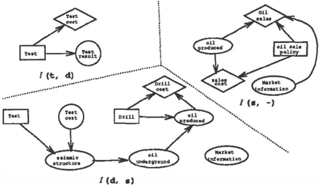
There are four sections in this SDID: I(-, t ) , I(t, d), I ( d, s ) , and I( s ,-) . The initial section I (-, t ) is empty. All the other sections are shown in Fig. 3.

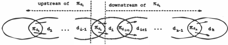
The concept of sections provides us with a perspec­ tive of viewing smooth regular SDID's. A smooth regular SDID I can be thought of as consisting of a chain sections I(-, d1), I(d1, d2), ... , I(dk-1, dk), and I(dk,-). Two neighboring sections I(di-l,di) and I(d;, di+l) share the nodes in 7rd,, which m-separate the other nodes in I(d;_1,d;) from all the other nodes I(d;, d;+l)· Fig. 4 shows this abstract view of a smooth regular SDID.

In the extended oil wildcatter example as shown in Fig. 3, the sections I( t , d ) and I ( d, s ) share the nodes test and test-result, and the sections I( d , s ) and I( s -) share the nodes oil-produced and market-in:formation.

3.3 CONDITIONAL PROBABILITIES AND LOCAL VALUES IN THE SECTIONS

In the section I(d;, d;+1), there is no decision node out­ side 1r d; U { di}. The value nodes are at leaves by defini­ tion. So, one is able to compute the conditional prob­ ability PI(d;,d;+1)(1rd;+1/7rd,, d;) of the nodes in 7rd; + 1 given the nodes in 1r d; and d;. We shall refer to this probability as the conditional probability of 1rd ;+1 given 1rd; and d; in I.

In the initial section I(-, d1), one can compute the probability PI(- , d1l7rd1). We shall refer to this prob­ ability as the prior probability 1r1 in I.

For a value node Vj in I(d;, d;+l), one can compute conditional probability PI(d;,d;+1)( 1rv i l 1r d., d;). Define

where fv; is the value function of Vj in I.

Let v1, . . . , Vm be all the value nodes in the section I(d;, di+1)· The local value function f;: n,.d· X n d , -n of the section I(d;, d;+t) is defined by I

When there are no value node in the section, then /; is defined to be the constant 0.

We can also define the local value "function" for the initial section, which is not really a function, but just a constant. We shall denote this constant by f o .

3.4 CONDENSATION

Intuitively, condensing a smooth regular SDID I means to do the following in each section I(d;, d;+l) of I: (1) getting rid of all the random nodes that are neither in the 7r d; nor in 7rd ' + " (2) combining all the value nodes into one single value node vf, and (3) col­ lecting the nodes in 1r a, into one compound variable x;. This results in a Markov decision process.

Now the formal definition. The condensation of I, de­ noted by Ic, is defined as follows:

1. It consists of the following nodes:
2. Random nodes x; (0:::; i:::; k), where x; is the compound variable consists of all the nodes in 1ra, when 71' d , =/= 0. When 7rd ; = 0 or when i = 0, x; is a degenerated variable that has only one possible value, say, o 1 .
3. Value nodes vf (0 :::; i:::; k ),
4. The same decision nodes d; ( 1 :::; i :::; k) as in I; and
5. The graphical connections among the nodes are as follows:
6. For any i E {2, 3, . . . , k }, there are two arcs converging at x;, one from Xi-1 and the other from di-1·
7. For any i E {1, 2, . . . , k }, there is an arc from x; to d;,
8. For any i E {1, 2, . . . ,k}, there are two arcs converging at vf, one from Xi and the other from d;.

1 The presence of the node xo makes the picture ugly. But we need it for two reasons. First, there may be value nodes in the initial section. Second, we want to be able to talk about the condensation of an influence diagram that contains no decision nodes.

• There are two arcs emitting from Xo, one to vg and the other to x1.
• The conditional probabilities and value functions are as follows:
• The conditional probability pe( Xi+llx;, d;) (i E {1, . . . ,k1}) is defined to be PI(d;+l,d;)(7rd;+ll 7rd., d;);
• The conditional probability pe(x1!xo = <> ) is defined to be PI( - , d l ) ( 1r d ,), and the probabil­ ity pc( x0) is trivially defined since x0 takes only one value <>;
• The value function fv� for vf (i E {0, 1, . . . , k}) is defined to ' be /;.

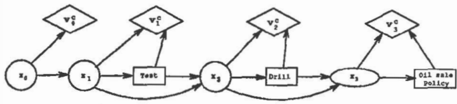
Fig. 5 depicts the condensation of the SDID shown Fig.2. Since test has no parent, x1 is a degener­ ated variable. The variable x2 stands for the com­ pound variable consisting of test and test-cost, and X3 stands for the compound variable consist­ ing of oil-produced and oil-market. The condi­ tional probability pe(x3lx2, d ) , for instance, is the con­ ditional probability P J(d , s) ( op, mi It, tr, d ) of op and mi given t, tr, and din the section I(d, s).

The value function fvc for the value node vf is a representation of tes 1 t-cost, fv � is a representa­ tion of drill-cost, and fvc is a representation of 3 oil-produced and sale-cost.

There is no value node in the initial section. So fvo is the constant 0. The node is kept only for uniformi t y.

Two decision networks are equivalent if they have the same optimal value and share the same optimal poli­ cies. The following theorem is proved in Zhang (1993).

Theorem 1 A smooth regular SDID is equivalent to its condensation.

To end this section, we would like to echo what we said at the beginning of the section. The process of con­ densing a SDID only involves two types of operations: the operation of computing conditional probabilities and the operation summing up functions (see subsec­ tion 3.3). The latter is straightforward. The formmer can be carried out by by any well established Bayesian network evaluation algorithm. One advantage of the concept of condensation is that it leads to a simple way of implementing influence diagrams on top of a system for Bayesian network computation.

4 COMPUTING THE VALUE OF PERFECT INFORMATION

Let I be a regular SDID. Let d3 and c respectively be a decision node and a random node in I, such that there is no arc from c to d8 in I. Let I' be the diagram obtained from I by adding arcs from c to d3 and to all the subsequent decision nodes. If there is no direct cycles in I'2, then I' is again a regular SDID. In such a case, the value of perfect information on c at d3 in I is defined to be the difference between the optimal expected value of I' and that of I.

In the following, we shall use 71'� to denote the set of parents of d in I'.

To determine the value of perfect information on c at d8, one needs to compute the optimal expected val­ ues of both I and I'. To this end, we adopt the two stage approach described in the previous section, i.e we first compute the condensations of I and I', and then evaluate the condensations respectively. An ad­ vantage of this approach is that it can make use of in­ formation stored in the condensation of I in comput­ ing the condensation of I'. More explicitly, for each section I(d;, di+1) of I, the conditional probability Pr(a,,a, + ,>{1l'a,+,l1l'a,, d;) and the local value function /; are computed and stored in the condensation of I. This paper seeks to make use of this conditional prob­ ability and this local value function in computing the conditional probability Pl'(d;,d;+1)(11'�· + 117l'd ; · d;) and the local value function ff of the corresponding sec­ tion I' ( d;, d;+1) of I'.

To see an example, 'let I be the SDID shown in Fig. 2. Consider the value of perfect informa­ tion on market-information at drill. In this case, I' is the same as I expect for the arc from market-information to drill. The section I'(s, -) is the same as I(s, -) . Thus, when computing the condensation of I', the conditional probability and the local value function for this section can simply be re­ trieved from the condensation of I.

The section I' ( t, d) is the same as I( t, d) except that u � tains one extra random node market-information. The node market-information is isolated in I'(t,d). In the condensation of I', one needs P1, (t,d) (mi, trlt). This can be computed by

where P(mi) is given in the specification of the diagram and PJ(t,d )(trlt) can be retrieved from the condensa­ tion of I.

The section I'(d, s) is also the same as I(d, s ) . How­ ever, the decision nodes drill has one more parent,

2It is always the case if the influence diagram is in the so-called Howard normal form. See Matheson (1990).

namely market-information in I' than in I. Thus, to obtain the condensation of I', one needs the conditional proba­ bility P1, (d , s )(op,mijt,tr,d,mi). In the condensation of I, one has PJ(d , s )( op, milt, tr, d). The nice thing is that one can easily compute P1, (d , s )(op,milt, tr, d, mi) from Pl' (d ,s)(op,milt, tr, d), which is the same as P J(d , s )(op,mijt,tr,d), which in turn can be retrieved from the condensation of I.

To summarize, it takes very little computation to ob­ tain the condensation of I' from the condensation of I. The rest of this section is to show that the same can be true for many other cases. We shall do this case by case. But first, some preparations.

4.1 REMOVABLE ARCS

A random node can be in more than one section. In the oil wildcatter example, market-information is in both the section I(d, s) and the section I( s, -) . Let dt be the last decision node such that c is in the section I(dt_1, dt) ( remember that there is a total ordering among the decision nodes ) .

The reader is advised to pay close attention to the definition of dt and the definition of d, ( given at the beginning of this section ) , ince we shall use them fre­ quently in the rest of the paper.

It follows from a result of Zhang and Poole (1992) that in I' the arcs from c to the decision nodes subsequent to dt, i.e to the decision nodes dt+b ... , dk are remov­ able, in the sense that the removal of those arcs results in an equivalent influence diagram. As a corollary, if t < s, all those arcs in I' that are not in I are remov­ able. Hence, I and I' are equivalent. In other words, if c is in the upstream of 71',, the value of perfect infor­ mation on c at d6 is 0. In the extended oil wildcatter example, it is of no value to acquire perfect knowledge about seismic-structure at the time one is to make the oil-sale-policy.

From now on, we shall let I' stand for the diagram after the removal of those removable arcs.

4.2 TWO ASSUMPTIONS

We assume that c is a root random node, i.e it has no parents. A consequence of this assumption is that if I is smooth, so is I'. When c is not a root, one can transform the diagram by a series of arc reversals so that c becomes a root in the resulting diagram. This is very similar to the operation of smoothing mentioned in subsection 3.1. See Zhang (1993) for details.

We also assume that dt_1 is a parent for every value node in the section I(dt-1, dt)· The assumption is to assure that if a value node appears in a section I( d ; , di+1) of I, then it appears in the corresponding section I'(d;, di+l) of I'. This a1lows us more chances in making use of the local value functions of the sec-

tions of I in computing the local value functions. of I', as the reader will see in the following. The assumption is not restrictive because one can always pretend that the value function f, of a value node v in I(dt-1. dt) depends on dt even thought it actually does not.

Under those two assumptions, we can show that I'(dj,dJ+t) is the same as I(dj,dJ+1) except that it may contain the extra random node c.

4.3 SECTIONS BEFORE da-1 AND SECTIONS AFTER dt

We need to consider four cases. Let us first discuss the easiest case: the sections before d·-1 and sections after dt.

This case occurs when i � s-2 or i"?:t. In such a case, I'(d;,, d£+1) is exactly the same as I(d;,, d;,+l)· So, the conditional probability and the local value function in I'(d;,, d£+1) are the same as those in I(d;, d;+l), which can simply be retrieved from the condensation of I.

In the extended oil wildcatter example, the terminal section falls into this category.

4.4 THE SECTION FROM da-1 TO d.

The section I'(da-1> d,) is the same as I(d·-1. d,), ex­ cept that it contains one extra node c. This node is isolated in I' ( d,_1, d.). Thus c is independent of all the other nodes in I'(d.-1, d,).

Since 7ra , _ , = 1r d,_, and 7r a , = 1r d, U { c}, the condi-. tional probability PI'(d,_, ,d,) ( ?ra , I?Ta , _ , , d a- 1) can be computed by

where equation (5) is due to the fact that c is inde­ pendent of all the other nodes in I'(ds-1> d.). In equa­ tion (6), P(c) is given in the specification of I and PI(d,_1,d,) (1Td,\1Td, _., ds-1) can be retrieved from the condensation of I.

We now turn to the local value function. For any value node v in the section I(d._1,d.), we have that c rt ?Tv , because c is in another section. By making use of the fact that c is independent of all the other nodes in I' (d s -1 > d8) again, we get

This equation and equations (3, 4) give us the following formula for computing the local value function /!_1 in the section I'(da-1 ,d 8 ) :

where fa-1 ( 1Td ,_1 , ds-1) can be retrieved from the con­ densation of I.

In the extended oil wildcatter example, the section from test to drill falls into this case.

4.5 SECTIONS IN BETWEEN d. ANDdt-1

This subsection considers the case when s < i < t -1. In this case, the section I'(d;, d;,+1) is t h e same as I( d;, d;,+l), except that it contains one extra node c. This node is isolated in I'(d;,, d£+1). So, c is in­ dependent of all other nodes in I'(d1, d;,+1). Since 1r d ; == 1r d; u { c} and ?ra ;+ < = ?T d;+1 u { c}, the condi­ tional probability pl'(d;,d i+l ) ( 1r a i+l 1 1r a ; ' d;,) satisfies

where PI(d;,d;+1)( 1T d;+1\?T d; , d;,) can be retrieved from the condensation of I since c E 1r d , ·

We now turn to the local value function. For any value node v in the section I(d;, d;+l), we have that c � 1r ,. By making use of the fact that c is independent of all the other nodes in I'(d;, di+l) again, we get

This equation and equations (3, 4) give us the following formula for computing the local value function ff in the section I'(d;, d£+1):

where / ;( 7rdi> d;) can be retrieved from the condensa­ tion of I.

4.6 THE SECTION FROM dt_1 TO dt

This subsection considers the section from dt-l to dt. The section I'(dt-1> dt) is the same as I ( dt-1> d t ) , and ?T a ,_, = 'lT d,_, U {c} and ?T a , = 1rd, · Thus we have

If c E 1r d, , we have

Thus, one can use the right nand side of equation (10) to compute PI'(d,_1,d,)(1rd,l1Td,_,,dt -d whencE 7rd,· In the extended oil wildcatter problem, the section from drill to oil-sale-policy is an example of this case.

On the other hand, if c rJ. 1Td,, there is no obvious way to make use of P1(d,_1,d,)(1rd, l7rd,_1, dt-d in com­ puting Pl'(d,_1,d,)( 1rd, i 1Td 1_ 1 , dt-d· In such a case, PI'(d,_1,d,)(1rd,i1Td,_1 , dt-1) needs to be computed from scratch.

Now, the local value function. If for every value node v in the section I( dt-1, dt), one has that 1r1J � 1Td1_1 U {dt-d, then it is easy to see that

Again in the extended oil wildcatter problem, the sec­ tion from drill to oil-sale-policy is an example of this case.

In any other case, we see no way to make use of ft-1 in computing JI_1. One needs to compute fi_1 from scratch.

4. 7 How much computation savings?

To end this section, we would like to give the reader some idea about how much computation our approach can save. There are two SDID's, the original I and the modified I'. The savings are in the process of evalu­ ating I'. There are two stages: in stage 1 one con­ denses I', and in stage 2 one evaluates the condensed SDID. As we have shown in this section that it takes very little computation to obtain the condensation of I' from that of I. This means a lot of savings if there are many random nodes in I that are not parents of any decision nodes, since those are the nodes that the condensation precess needs to get rid of. As we have pointed out earlier, our approach is especially useful if one wishes to evaluate the value of perfect information for a number cases. One can compute the condensa­ tion of I once and use it for all the cases. We can also save some computation in stage 2. Since I'(d;, di+1) and I(di, di+1) are the same for all i 2: t, we need not to re-evaluate these sections at all. Furthermore, we can save more if we adopt a top down approach for evaluating the condensed diagrams. See Qi (1993) and Zhang, Qi, and Poole (1993'a) for details.

5 CONCLUSIONS

The value of perfect information in an influence dia­ gram is defined as the difference between the optimal expected value of a properly modified influence dia­ gram I' and' that of the I itself. In this paper, we have described a method for computing the value of perfect information. The method is incremental in the sense that it computes the value of I' by using the in­ termediate computation results obtained in evaluating

1. Of fundamental importance to the method is the concept of condensation, which also leads easy imple­ mentations of SDID's on top of a system for Bayesian network computations.

Acknowledgement

This paper is partly supported by NSERC Grant OG­ P0044121.

References

1. V. Denardo (1982), Dynamic Programming: Models and Applications, Prentice-Hall.
2. A. Howard, and J. E. Matheson (1984), Influence Diagrams, in The principles and Applications of Deci­ sion Analysis, Vol. II, R. A. Howard and J. E. Math­ eson ( eds.). Strategic Decisions Group, Menlo Park, California, USA.
3. L. Lauritzen and D. J. Spiegehalter (1988), Local computations with probabilities on graphical struc­ tures and their applications to expert systems, Journal of Royal Statistical Society B, 50: 2, pp. 157 - 224.
4. E. Matheson (1990), Using influence diagrams to value information and control, in R. M. 0 liver and J. Q. Smith eds. (1990), Influence Diagrams, Belief Nets and Decision Analysis, John Wiley and Sons.
5. Qi (1993), Decision Graphs: algorithms and appli­ cations, Ph.D Dissertation, forthcoming.
6. Qi and D. Poole, Decision Graph Search, technique report TR-93-9, Department of Computer Science, the University of British Columbia. This paper has been submitted to a journal.
7. Raiffa, (1968), Decision Analysis, Addison-Wesley, Reading, Mass.
8. Shachter (1986), Evaluating Influence Diagrams, Operations Research, 34, pp. 871-882.
9. Zhang and D. Poole (1992), Stepwise-decomposable influence diagrams, in Proceedings of the Fourth Inter­ national Conference on the Principles of Knowledge Representation, Oct. 26-29, Cambridge, Mass.
10. Zhang, R. Qi and D. Poole (1993a), Minimizing De­ cision Tables in Influence Diagrams, in The Proc. of the Fourth International Workshop on Artificial Intel­ ligence and Statistics, Ft. Lauderdale, Florida, Jan­ uary 3-6, 1993.
11. Zhang, R. Qi and D. Poole (1993b), A computa­ tional theory of decision networks, technical report TR-93-6, Department of Computer Science, the Uni­ versity of British Columbia. This paper has been sub­ mitted to The International Journal a/Approximate Reasoning.
12. Zhang (1993), A computational theory of decision networks, Ph.D Dissertation, under preparation.