Independence with Lower and Upper Probabilities

Lonnie Chrisman School of Computer Science Carnegie Mellon University Pittsburgh, PA 15217 [email protected]

Abstract

It is shown that the ability of the interval probability representation to capture episte­ mological independence is severely limited. Two events are epistemologically indepen­ dent if knowledge of the first event does not alter belief (i.e., probability bounds) about the second. However, independence in this form can only exist in a 2-monotone probabil­ ity function in degenerate cases- i.e., if the prior bounds are either point probabilities or entirely vacuous. Additional limitations are characterized for other classes of lower prob­ abilities as well. It is argued that these phe­ nomena are a matter of interpretation. They appear to be limitations when one interprets probability bounds as a measure of epistemo­ logical indeterminacy (i.e., uncertainty aris­ ing from a lack of knowledge), but are ex­ actly as one would expect when probability intervals are interpreted as representations of ontological indeterminacy (indeterminacy in­ troduced by structural approximations).

1 Introduction

Let (!J, :F) be a probability space, and let E. , P :F --+ [0, 1] be set-functions on this space satisfy­ ing the following properties for any A, B E :F with An B = 0:

where A denotes !JA, the complement of A. Then P and P are called lower and upper probability functions respectively. It is always the case that P (A):::; P (A). It is only necessary to store one or the other of E. and P , since each can be obtained using Property 2 once the other is known. The lower and upper probabil­ ity envelopes of a non-empty set of distributions P on en 1 :F) are functionS

Every lower (upper) probability envelope is a lower (upper) probability. Thus, the lower probability rep­ resentation provides a convenient description of a set of distributions.

A number of uses have been suggested for lower prob­ abilities, and their use is rapidly increasing. Some feel that the use of a single exact distribution in Bayesian­ style inference fails to satisfactorily distinguish be­ tween uncertainty and ignorance or between certainty and c on fid e nc e , and t h er e f o r e a more gene r a l repre­ sentation such as lower probability functions may be a superior representation of belief [21, 22, 24, 32, 33]. Lower probabilities may also arise from incomplete or partial elicitation, such as when insufficient knowledge is available, or when it is too time consuming to obtain obtain the necessary knowledge to warrant the preci­ sion inherent in exact probabilities [2, 16, 18]. Lower probabilities are also useful for studying sensitivity and robustness in probabilistic inference [1, 36, 40], and they can be used to weigh computation effort against modeling precision [9]. They arise in group decision problems [24, 28] and in axiomatic approaches to un­ certainty when the axioms of probability are weakened [17, 26, 33, 36]. They arise when determining con­ straints on probabilities given only the probabilities on a finite set of other events [14, 27]. Finally, they may result from the abstraction of more detailed prob­ abilistic models [5, 6, 19].

This paper examines a particular problem that arises with the use of lower probability functions when we at­ tempt to model independent events. We limit our con­ sideration to Bayesian-style updating of lower proba­ bility functions, such that when evidence E C Q is learned, each distribution in P is updated according to Bayes's rule, yielding the new updated bounds

It is often impossible to capture epistemological m­ dependence within a lower probability representation ([36] uses the term epzstemic independence. Here we follow [37] by using the term epistemologica0. Two events being epistemologically independent would im­ ply that learning the truth about the first should not alter belief (i.e., probability bounds) on the sec­ ond. Specifically, if the initial lower probability is 2monotone (defined later), we show that epistemologi­ cal independence cannot be captured unless we are in one of the degenerate cases where P = P (i.e., the point probability case) or P = 0 and P = 1 (the vac­ uous case). We also characterize other circumstances in which a lower probability cannot capture this type of independence.

We argue that the apparent inability of lower proba­ bilities to capture independence is a matter of inter­ pretation. Although we have specified that the bounds arise as extrema of P, we have not specified why a set of distributions should be considered in the first place. The apparent difficulty arises from an implicit assump­ tion that the set of distributions is used to represent some form of epistemological indeterminacythat is, a degree of knowledge or the lack of knowledge about the true situation. The qualitative properties of the lower probability representation, particularly with re­ spect to representing independence, but also in terms of related phenomena such as dilation [ 2 9 ] , make it poorly matched for epistemologically-based interpre­ tations. We propose instead an alternative interpreta­ tion, whereby the bounds arise as a result of ontological (i.e. , structural) considerations. In our interpretation, (point) probabilities capture the epistemological inde­ terminacy, but ( approximate ) structural assumptions placed on a model from above introduce additional in­ determinacy with a qualitatively different nature, one in which the behavior of the bounds under condition­ ing can be logically interpreted.

2 Coin Tossing Example

Suppose we have two coins which we consider to be physically independent of each other. We are going to toss both coins and observe their outcomes. Each coin has only two possibilities, {heads , tails}, and each has its own (unrelated) bias on the probability of landing heads, which we know only to be between 1/4 and 3/4. First , we wish to characterize our knowledge using a lower probability function. We denote the four possi­ ble outcomes as n = {hth2, hti2, ith2, iti2}·

Since it may be the case that both coins have a 1/4 probability of heads, we assign E._({h1h2}) = 1/16. Similarly, they may both have a 3/4 probability of coming up heads, so we assign P ({h1h2}) = 9/16. Carrying out this logic for all of the 16 possible sets of outcomes, we obtain the bounds in Figure 1.

Let P( P ) denote the set of all probability distribu­ tions consistent with the bounds in Figure 1 -i.e.,

For the sets:	p	p
f/J	0	0
{h1h2J, {h1t2}, {t1h2}, or {t1t2}	1/16	9/16
{hth2,htt2}, _ {ith2,itt2}, {hth2, ith2} or {h1t2, t1t2}	1 4	3 4
{h1h2,t1t2} or {h1t2,t1h2}	3/8	5/8
thlt2,ith2,iti2�. {hth2,ith2, iti2}, {h1h2,h1t2, t1t2}, or {h1h2,h1t2,t1h2}	7 I6	15 16
n = {h1h2,h1t2,h2t1.t1t2}	1	1

F ig u r e 1: Bounds on the possible joint outcomes of two coins.

For the sets:	p	p
1/J, {t1h2}, {t1t2}, or {t1h2,t1t2}	0	0
thth2}, {hti�}, {hth2,ithd {hti2 , iti2}, {hth2,iti2}, {hti2, ith2} {h1t2,t1h2,t1t2}, or {h1h2,t1h2, t1t2}	1 8	7 8
thth2, htt2}, { _ hth2,hti2, tlt2}, {hth2,h1t2, t1h2}, or Q = {hth2,hti2,tth2,tlt2}	1	1

Figure 2: Bounds after conditioning on H1 {hth2, htt2}-

Suppose we observe the outcome of the first coin to be heads without observing the outcome of the sec­ ond coin. This gives us the conditioning event H1 = {h1h2, h1t2}· We then update our bounds given the new evidence as follows:

This yields the new bounds shown in Figure 2. Notice the new bounds for the event H2 = {hth2, t1h2}, which were previously [1/4, 3/4], but are now [1/8, 7/8]. The outcomes of the two coins are supposedly indepen­ dent, yet learning the outcome of the first coin had a marked influence on our beliefs about the outcome of the second (independent) coin. The representation has clearly failed to capture the independence.

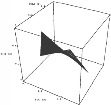
The inability to capture this independence is related to the fa c t that P(P ) includes distributions in which the coins are not independent. Using the set

would more accurately reflect the complete knowledge in this example. This is what [36] calls the sensitivity analysis approach to independence, and [11) call type1 independence. This (non-convex) set of p ro b a bi l i tie s is shown graphically in F i gu re 3. For this set, P (Hz),

as defined by ( 1) and shown in Figure 1, is equal to P (H2IH1), as defined by (2), so a perfect representa­ tion of P would capture the independence. However, a primary reason for studying the lower probability representation is for the purpose of using it as a com­ plete representation of belief. Because independence plays a central role in many theories of subjective be­ lief, the fact that the lower probability representation has problems capturing independence is significant. In the remainder of the paper, we will characterize this (in)ability to capture independence and examine what this suggests for the interpretation of the representa­ tion.

3 Lower Probability

Before examining the independence issues in more de­ tail, this section defines some notation and reviews some of the basics of the lower probability repre­ sentation. The subsequent section characterizes in­ dependence issues. The properties and terminology in this section has been developed and utilized by [ 3 , 4, 7, 36, 37] and others.

A lower probability is a function obeying the proper­ ties listed in the introduction. A probability distribu­ tion, P, is consistent with a lower probability P if for every A E :F, P (A) :S P(A). We denote by P(P ) the set of all distributions consistent with £ . The con­ ditions in the introduction are not strong enough to ensure that P(P ) i= 0. A lower probability P1 domi­ nates P2 if for all A E :F, P1 (A)� P 2 (A) ;in which case P(P 1 ) c P(P 2 ). --

Denote the lower probability envelope P obtained from P using (la) by P [P]. It does not follow that P(E_ (P]) = P. In other words, many different sets of distributions share the same bounds. The set P(P [P]) is called the maJ·arization of P. When P ( P [P]) = P, P is said to be closed to majorization ([39]). When P = P , then P is a probability distribution.

Every lower probability function is monotone (some­ times called 1-monotone), meaning that P (A) :S P (B) whenever A C B. A stronger property called 2-monotonicity is often usefuL A lower probability E._ is 2-monotone when for every A, B E F,

Two-monotonicity is a sufficient (but not necessary) condition to ensure that £ is a lower envelope. Two­ monotonicity is usually necessary for obtaining ex­ act dosed-form m ani p u la tion formula, and is therefore usually assumed in practice.

The lower and upper probabilities conditioned on event E E :F are given by

It is well-known [7, 13, 15, 38, 39] that when E. 1s 2-monotonc,

whenever £ (E) > 0, and P (AlE) = 1 whenever A C E and P (E) > £(E) == 0. If P (E) = 0, then the conditional lower probability is undefined.

Let f2 be finite, :F = 2°. The Mobius transform of P is a set function m : :F --+ lR defined by ((30, pg. 391)

If m(A) � 0 for all A E F, then P is said to be a belief function. Belief functions are used by the Dempster-Shafer theory ([30]) and in the Transferable Belief Model ([32]), but in those theories are given ev­ idential interpretations rather than the lower proba­ bilistic interpretation of interest here (see [20] and [31] for good discriptions of the difference). Belief func­ tions are also what [4] terms infinitely-monotone ca­ pacities ([34]). Every infinitely-monotone lower prob­ ability (i.e., belief function) is also 2-monotone, but the converse does not hold.

The Mobius transform is information preserving, so that the original function can be recovered from m

using the inverse Mobius transform, given by

Subsets A E F with m (A) -=f 0 are called the focal elements of P .

Let P A and PB be lower probabilities on 0 A and OB respectiveV. The meta-Markov combination of P A and P B ([10]), denoted P = P (P A ) @ P(PB ), is the set of distributions on 0 = 0 A ---x-?lB given by

This is the set consisting of all independent events, i.e., the set shown in Figure 3 for the coin tossing example. We also write P = P A @ PB for the majorization of this set. --

4 Representation of Independence

Probabilistic independence of A and B is characterized by either of two properties:

In the case of a probability distribution each of these imply the other. It is not hard to see that in the case of lower probabilities the two properties do not imply each other, and therefore it seems natural to define independence for lower probabilities as the conjunc­ tion of both properties, i.e., A and B are independent whenever

In fact, [37] give exactly this definition. However, as the subsequent theorems show, the two are often mu­ tually incompatible.

Theorem 1 When P is 2-monotone, the following conditions cannot all hold:

where P (A/B) = inf {P (A/B) : P E P(P ), P(B) > 0} and A, B C fl. If any one of the four properties is removed, the three remaining properties can co-exist.

The above shows that a 2-monotone lower probability cannot exhibit the desired properties of independence except in the degenerate cases where P (A) = 0 or P ( A)= 1, i.e., when P is entirely uninformative (vac­ uous) about A, or when P (B) = P (B) (i.e., P (B) is a point probability on B).

We can demonstrate the applicability of the above the­ orem on the following example.

Example 1: [The Extended Monte Hall Problem) Jane is a contestant on Let's Make a Deal, a game show. Presented with four curtains, behind only one of which is a prize, she selects Curtain 1. The host then reveals first that there is nothing behind Cur­ tain 4, and second that there is nothing behind Cur­ tain 3. Making the assumptions that initially the lo­ cation of the prize is equiprobable, that the host will always show two empty unselected curtains, that the unselected curtain not revealed is chosen uniformly, that the curtain order is independent of all other as­ pects of the problem, and that her knowledge about how the curtain order is picked is characterized by a vacuous lower probability, what is the lower prob­ ability of winning if she does not change her selec­ tion? What is the lower probability of winning if she does change selection? Assume Jane initially captures all the knowledge of the problem using only a lower probability distribution, and that the frame of dis­ cernment used includes the curtain order (so that n = {123,132,124,142,134,143,234,243,324,342,423,432} where ijk abbreviates "the prize is behind i, the host reveals first j and second k).

The information stated above is encoded in the lower probability function with the Mobius transform focal elements

The initial lower probability is in this case a belief function, and therefore 2-monotone. Conditions 1, 2, 4, and 5 of Theorem 1 are satisfied, so by observing the order in which the curtains are revealed, we know her lower probability for each of the two questions is effected. In particular, after observing the revealed curtains and their order, her remaining belief becomes vacuous, i.e.,

Had she ignored curtain order entirely, using fl = { 12, 13, 14, 21, 31,41}, where ij abbreviates "the prize is behind i , the host does not reveal j , " her final be­ liefs (according to Bayes's rule) are that she'd have a point-probability of 3/4 of winning if she changes her selection, or a point-probability of 1/4 if she does not change. Once again, the result should be com­ pletely independent of the curtain order, but in the

lower probability representation the influence can be quite dramatic. D

Theorem 1 covers a wide class of lower probabilities that are of great interest. However, there are in ad­ dition lower probability functions that are not even 2-monotone, but for which independence properties cannot hold. The lower probability in the initial coin tossing example (Figure 1) was such an example - it is not 2-monotone. Therefore, it is possible to obtain further characterizations for when the independence properties cannot co-exist. The following characteri­ zation covers the coin tossing example.

Theorem 2 Suppose P(£. ) is the set of distributions consistent with E. I and let A, B c n. If there exists a P E P(P ) such that P(A) = P (A), P(B) > 0 and P(A) > P(AIB), then P (A) > P (AlB).

Dually, if there exists a P E P(P ) such that P(A) = P (A) and P(A) < P(AIB)� then P (A)< P (AlB).

That Theorem 2 covers the initial coin tossing ex­ ample is immediately seen with the distribution (1/16, 3/8, 3/16, 3/8), which is consistent with the bounds in Figure 1 and satisfies the conditions in The­ orem 2.

Theorem 2 is closely related to [29, Theorems 2 and 3] which state virtually identical conditions under which B will dilate the lower probability bounds (i.e., the posterior bounds after updating on B will strictly con­ tain the prior bounds). Clearly, if the bounds dilate on an event that is supposed to be independent, the lower probability is not exhibiting the independence properties. However, the connection between dilation and independence is actually closer than this. For ex­ ample, [29, Theorem 1] shows that dilation can only occur if the set of distributions with the desired in­ dependence property intersects the set of consistent distributions. The following theorem emphasizes this connection between the independence properties and dilation - independent events cannot cause a set of independent distributions to contract.

Theorem 3 Let P = P A @ PB 1 with P (AlB) given by (2). (Similarly for P ). Then for A = A' X nB and B = n A X B', where A' c nA and B' cOB:

In addition to the connection with dilation (Items 3 and 4), Items 1 and 2 of Theorem 3 demonstrate that the factorization property of independence is always a property of lower probabilities when we are dealing with independent events. Recall that these conditions appeared in Theorem 1.

The idea that information about one fact should not influence beliefs regarding certain other facts is an im­ portant component in many formalizations of knowl­ edge representation. The theorems in this section demonstrate that the lower probability representation often cannot exhibit this property except in degenerate cases.

An alternative version of epistemological independence is possible. Instead of requiring that independent events do not affect conditioned probability bounds, events can be called independent whenever P (AlB) :::; P (B). This version is identified by [12, Definition 4.3] with the rationale that independent events should not contribute additional information, a requirement that is much weaker than the irrelevance requirement. This weaker requirement is compatible with the factoriza­ tion property and, as evidenced by the results of this section, is a preferable property for independence within the lower probability framework. It also should be noted that while [37] define independence as hav­ ing both properties hold, [36] defines epistemological independence as the first property (irrelevance) only.

5 Abstraction

This section examines factorization and the relation­ ship between a factored lower probability and its con­ sistent probability distributions. This relationship is central to the interpretation of lower probability con­ sidered in the subsequent section.

Let P* be an arbitrary probability distribution on 0 = n A X nB. Specifically, it is not necessarily the case that A ll B [P*] (that A is independent of B with respect to P*).

Definition 1 A lower probability P on 0 is an ab­ straction of P* relative to the assertion A ll B when

where p A is a lower probability on n A I PB is a lower probability on OB. P is a proper abstraction if it is not dominated by any other abstraction of P* relatzve to A ll B.

It is worth emphasizing that an abstraction is factoriz­ able (Item 2) and captures information about p· with­ out introducing information that is not implied by P*. No abstraction can capture strictly more information than a proper abstraction without introducing infor­ mation that is not implied by p·; however, a proper abstraction is not unique - there may be an arbitrar­ ily large number of proper abstractions relative to a single independence assertion, and each of these may contain information not contained by the others. Note that by definition, any abstraction is closed to ma­ jorization.

Theorem 3 has already revealed that P (A n B) = P (A)P (B). This does not, however, describe the lower probability of non-rectangular sets ( those which cannot be written as Ax B). The full characterization of all sets is most conveniently stated in terms of the Mobius transform.

Theorem 4 If P is an abstraction of a distribution P relative to A Jl B , and m is the Mobius transform of P, then

Theorem 4 does not reqmre the abstraction to be proper.

It is possible to generalize the concept of an abstrac­ tion relative to a single independence assertion to the concept of an abstraction relative to a set of con­ ditional independence assertions. This introduces a number of complications beyond the scope of the cur­ rent paper. A general concept of factorization ( decom­ position ) of lower probabilities is developed in [8].

The concept of a proper abstraction immediately suggests an interpretation for probability bounds namely, that a lower probability is an abstraction of some ( more detailed ) probability distribution. The ex­ act identity of this distribution is lost - it is known only to be in P(P ) . The next section develops this interpretation.

6 The Ontological Interpretation

This section introduces an interpretation of lower probability. This interpretation resolves many of the apparent limitations discussed above, and provides an interpretation that suggests important uses for lower probabilities.

Let us assume that a probability or a lower probabil­ ity function is to serve as a model of some system or phenomena, as is often the case. Models are by their very nature approximations or abstractions of the ac­ tual system being modeled, and as such they bring with them a certain amount of indeterminacy. By in­ cluding probabilities or lower probabilities in the de­ scription of the model, we often aim to quantify this indeterminacy explicitly.

Constructing a model of a system involves two basic steps: (1) Choosing an ontology, and (2) Filling in the knowledge required by the ontology. An ontol­ ogy specifies the language used to describe the system, as well as structural and parametric assumptions that are built into the model. We can think of an ontol­ ogy as identifying a set of parameters that must be filled in to specify the actual knowledge of the partic­ ular system being modeled, as well as a set of variables that are used to describe particular problem instances. The ontology ( alone ) leaves the values of the param­ eters unspecified, for this is the epistemological infor­ mation. Once the parameters are specified, the model is completely specified, and the ontology relates these parameters to each other and to the problem instance variables. We refer to these two levels as the ontologi­ cal level and the epistemological level.

In the case where two coins are tossed, choices at the ontological level include assuming that exactly one of only two possible outcomes can occur for each coin, that the outcome of each coin can be characterized by a single probability, that outcomes of consecutive tosses are independent of one another and of the other coin. These correspond to choices of language, parametric assumptions, and structural assumptions respectively. This ontology requires two parameters to be filled in to completely specify the model. The values for the two coins' biases are the knowledge at the epistemological level.

Indeterminacy in a model can arise at either level, and we refer to these as ontological indeterminacy or epis­ temological indeterminacy ( these terms were coined by [37]). However, ontological indeterminacy can only ex­ ist when there is epistemological indeterminacy, be­ cause otherwise our model is nothing more than an exact description of the true situation.

Probability provides a very good representation for epistemological indeterminacy. We argue, therefore, that ( non-point ) lower probabilities are inappropri­ ate for quantifying pure epistemological indetermi­ nacy. This viewpoint is much along the lines of a strict "Bayesian" interpretation of probability, and in stark contrast to epistemological interpretations of proba­ bility bounds offered by [18, 20, 21, 23, 24, 25], and others, in which imprecision arises from a deficiency of knowledge or training data. Under our proposed inter­ pretation, interval probability bounds arise only as a result of ontological indeterminacy, i.e., structural as­ sertions that are only approximately true. Thus, when given a lower probability function, we immediately in­ terpret non-point intervals as a reflection of ontologi­ cal indeterminacy, and probabilities as a reflection of epistemological indeterminacy.

The relationship between epistemological and ontolog­ ical indeterminacy can be visualized as follows. The epistemological indeterminacy of a rational, coherent agent is quanitified by a probability distribution P*. p· can be thought of as the agent's deepest beliefs, but these might not be easily accessible to a resource­ bounded agent. Inferences are performed using a model that includes ontological assumptions conve­ nient for the problem ( s ) being solved. The model used by the agent is an abstraction of P* relative to the on­ tology's independence assertions. Ideally it is a proper abstraction so that a minimal amount of additional in-

determinacy is introduced by the abstraction.

It has been said that "the assumption of conditional independence is usually false" (35). By asserting a con­ ditional independence assertion, an agent is more typ­ ically asserting a belief that two events a r e almost con­ ditionally independent given a th i r d. An agent might assume, for example, that gravitational acceleration is independent of an object's height because it results in a useful model, even though deep down at the epistemo­ logical level the agent does not believe they are truly independent. The result of this structural approxima­ tion is that ontological indeterminacy is introduced.

6.1 Coin Tossing Revisited

It is instructive to apply this interpretation to the coin tossing example considered earlier. Consider the prob­ ability distribution, P*, given by

This probability distribution quantifies epistemologi­ cal indeterminacy. Since there is no structure (i.e., no independence or parametric restriction), there is no ontological indeterminacy, so the point probability on the joint space captures all the agent's uncertainty. If a rational agent had unlimited time and resources to access and compute the ramifications of its deep­ est beliefs, P* is the full assessment of beliefs it would obtain.

However, suppose the agent models the coins as in­ dependent. From (7), it is clear the agent does not really believe the coins to be independent - this is a structural approximation. There are several possible rationale for the agent imposing this artificial struc­ ture on its model: to simplify (factorize) computation, to reduce the number of parameters that must be as­ sessed, to obtain a structure that is better suited for explanation, to reason at different hierarchical levels of abstraction, etc.

The agent adopts (or subjectively estimates) a proper abstraction of P* relative to this independence asser­ tion. An infinite number of proper abstractions are possible, one of which is obtained by setting P (H1) = E.. (H2) = P (T1) = E.. (T2) = 1/4, which is shown in Figure 4. The lower probability in Figure 1 contains Mobius assignments on two non-rectangular sets, but is otherwise comparable to the lower probability of Fig­ ure 4. In [12], de Campos and Huete call Figure 4 a type-2 product, and Figure 1 a type-1 product, and relate the two with their Proposition 3.6.

When inference is performed using E.. , one should not assume anything a b ou t p· except what is implied as a result of P being an abstraction of P*. So, for exam­ ple, P is also a proper abstraction of the distribution

For the sets:	p	p
ll'l	0	0
{h1h2}, {h1t2}, { t 1 h 2 } or {ht2}	1/16	9/16
{hlh2, hlt2},_{tth2, t l t 2 } , {hlh2, ith2} or {h 1 t 2 , t1t2}	1/4	3/4
{h1h2, ittz} or {h1t2, t 1 h2l_	1/8	7/8
thlt2, ith2, itt2t, {hth2, ith2, t l t2 },	7	15
{h1h2, h1t2, t 1t 2 } or { h 1 h 2 , h1t2, t1h2}	i6	16
= {hlh2, hlt2, ith2, itt2}	1	1

0

Figure 4: Bounds encoding ontological indeterminacy for two independent coins.

Any inference from P should be valid for P as well as for p·.

Suppose the agent observes the outcome of the first coin to be heads, w it hout observing the outcome of the second coin. P ( H 2 I H 1 ) should bound the conditional probability P(H21Ht) for any more de­ tailed probabilistic model, and the bound must be valid for any consistent distribution. For example, P*(H2IH1) = 7/8, but if P is the distribution of (8) then P ( H 2 I H 1 ) = 1/8. In full, the desired conditional lower probability is indeed that given by (3) and shown in Figure 2. In other words, under the ontological i n ­ terpretation of lower probability, the bounds that pre­ viously seemed to present a paradox are in fact the desired conditional bounds. These new bounds are guaranteed to be consistent wit.h any ( ontologically) more detailed model.

The apparent paradox with the coin tossing example of Section 2 only appears paradoxical because of an implicit assumption that the lower probabilities are representing a form of epistemological indeterminacy. By interpreting the intervals of a lower p r ob a b i lity as r e pres e ntin g ontological indeterminacy, the results of conditioning are precisely what we would expect and desire.

6.2 Monte Hall Revisited

In the Monte Hall example, observing the order in which curtains are revealed causes Jane's b e l i e f about the prize's location to change from a point probabil­ ity to total ignorance. This occurs despite the fact that curtain order is modeled as independent of the prize's location. This result, however, is quite reason­ able when the lower probability is given an ontological interpretation. We must assume that independence between curtain order and prize location is imposed in order to factorize the lower probability. Furthermore, they are not independent at the epistemological level, for if they were, the belief would be characterized by point bounds.

The lower probability of (6) is an abstraction of a more refined model in which the host encodes the exact lo­ cation of the prize with the selection of curtain order.

For example, if the prize is behind the lower numbered unrevealed curtain, the curtains opened are revealed with the lowest numbered revealed first. This more refined model is certainly consistent with (6), as is the one where the encoding is reversed.

By adopting the beliefs in (6), Jane must believe that deep down, given enough time and thought, she can figure out how the host encodes the prize's location. The vacuous bounds simply indicate that the use of a more detailed model is certainly warranted for this problem. The assertion that the identity of the curtain not revealed is independent of the order the curtains are revealed hardly an approximation- it is blatantly false - and as a result, vacuous bounds result.

7 Conclusion

Lower probabilities are utilized for a great number of purposes within the robust statistics and uncertain in­ ference communities.

However, the results here demonstrate that the rep­ resentation has significant limitations in its ability to represent epistemological independence, the idea that knowledge of one event should not influence belief about a second event. Theorem 1 showed that inde­ pendence of this type can never be represented by a 2-monotone lower probability unless the bounds are tight (i.e., a point probability), or the bounds are to­ tally vacuous. Theorem 2 shows that this limitation extends to an even wider class of lower probabilities, and Figure 3 suggests the limitations extend even to more general representations of convex sets of proba­ bility distributions.

These limitations almost appear to be paradoxical. However, they are only paradoxes when one interprets probability bounds as an indication of epistemological indeterminacy. For example, one often sees it said that lower probabilities are useful because point probabil­ ities require more precision than available knowledge warrants. The results deal a blow to epistemologi­ cal interpretations such as this. When lower probabil­ i t y is appropriately interpreted, these limitations and the unusual influence of independent events on prob­ ability bounds is entirely natural and fully consistent with the interpretation. The ontological interpretation says simply that epistemological indetermancy (uncer­ tainty due to lack of total knowledge) is appropriately represented by a pure probability distribution. When structural approximations are asserted, ontological in­ determinacy is introduced. The lower probability rep­ resentation captures this ontological indeterminacy.

Several other concepts of independence for lower and upper probabilities, as well as for more general sets of probabilities, are also possible ([11, 12]). There are also several possible types of products that can be formed from marginal lower probability representa­ tions, and these result in various relationships between independence concepts and product formula. These relationships are studied in [12] and [36, Section 9.3].

In some cases it may be appropriate for an agent to fully assess its epistemological indeterminacy, thus ob­ taining a probability distribution P*, and then only later abstract this to a lower probability relative to a more structured or simplified model. This form of hier­ archical reasoning can reduce the computational effort for solving specific inferences considerably. Further­ more, for any given inference, the bounds obtained give a quantitative indication of how much precision was lost by using the abstract model, and this in turn gives an indication of whether an answer from the current level of abstraction is sufficient. However, fully assess­ ing epstemological indeterminacy first is not entirely necessary. It is also conceivable that bounds them­ selves are subjectively estimated without first estimat­ ing P*, perhaps by considering only the most extreme situations that violate structural approximations. A precise interpretation is important when making such subjective assessments, since it provides a conceptual basis for chasing specific bounds.

Concepts of independence are central to probabilistic reasoning, and are especially important when it comes to scaling to large domains. A thorough understand­ ing of independence and how it can be properly utilized is equally important to lower probabilistic reasoning. The ontological interpretation may provide a useful foundation for utilizing abstraction and structural ap­ proximation in the context of probabilistic inference, ideas that are also important when scaling probabilis­ tic inference to very large domains.

Acknowledgements

I would like to thank Fabio Cozman for comments on a draft of this paper. The author was supported by NASA-Jet Propulsion Lab Grant No. NGT-51039. The views and conclusions contained within are those of the author and should not be interpreted as repre­ senting the official policies, either expressed or implied, of the U.S. government.

References

1. J. 0. Berger. Robust bayesian analysis: Sensitiv­ ity to the prior. J. Stat. Plan. Inf., 25:303-328, 1990.
2. [2) J. Cano, M. Delgado, and S. Moral. Propagation of uncertainty in dependence graphs. In R. Kruse and P. Siegel, eds., European Conference on Sym­ bolic and Quantitative Approaches to Uncertainty (ECSQA U)., pages 42-47, 1991. .
3. A. Chateauneuf and J.-Y. Jaffray. Some charac­ terizations of lower probabilities and other mono­ tone capacities through the use of Mobius inver­ sion. Math. Soc. Sci., 17:263-283, 1989.
4. G. Choquet. Theory of capacities. Ann. Inst. Fourier (Grenoble), 5:131-295, 1953.

1. L. Chrisman. Abstract probabilistic modeling of action. In J . Hendler, editor, 1st Int. Conf. on AI Plan. Sys. , College Park, MD, 1992.
2. L. Chrisman. Reasoning about probabilistic actions at multiple levels of granularity. In A A A I Spring Symposium Ser.: Decision­ Theoretic Planning, Stanford Univ., 1 994.
3. L. Chrisman. Incremental conditioning of lower and upper probabilities. Int. J. Approx. Reas. , 13(1):1-25, 1995.
4. L. Chrisman. Propagation of 2-monotone lower probabilities (a.k.a. Choquet capacities) on an undirected graph. In 12th Conf. Uncert. in A.J. , 1996.
5. F. Cozman and E. Krotkov. Quasi-Bayesian strategies for efficienL plau generation: Applica­ tion to the planning to observe problem. In 12th Con f. Uncert. in A. I. , 1 996.
6. [10) A. P. Dawid and S. L. Lauritzen. Hy pe r Markov laws in the statistical analysis of de c om p o s a bl e graphical models. Ann. Stat., 21(3) , 1 993.
7. [ 1 1) L. de Campos and S. Moral. Independence con­ cepts for convex sets of probabilities. In E le ve n t h Annual Conf. Uncert. in A .J. , Montreal, 1 995 . .
8. [ 1 2] L. M . de Campos and J . F. Huete. Indepen­ dence concepts in upper and lower probabilisties. In B. Bouchon-Meunier, et al. , eds. , Uncert. Int. Sys. , pages 85-96. 1993
9. [1 3] L. M . de Campos, M. T. Lamata, and S. M or a l . The concept of conditional fuzzy measure. Int. J. Intel/. Sys., 5(3) :237-246, 1990.
10. B. DeFinetti. Foresight: Its logical laws, its sub­ jective sources. In H.E. Kyburg, Jr. and H.E. Smokier, eds., Studies in Subjective Probability, pages 93-172. Wiley, 1964. Appeared originally in An na l e s de l 'Institut Henri P o i n car e , Vol. 7 ( 1 9 37). Translated by H.E. Kyburg Jr.
11. R. Fagin and J . Y. Halpern. A new approach to updating beliefs. Technical Report RJ7222, IBM Almaden Res. Cntr., Comp. Sci., 1989.
12. K. W. Fertig and J . S. Breese. Probability inter­ vals over influence diagrams. IEEE Trans. PAM!, 15(3):280-286, 1993.
13. F. J . Giron and S. Rios. Quasi-Bayesian be­ haviour: A more realistic approach to decision making? In J. M. Bernardo, et al ., eds., Bayesian Statistics, pages 17-38. Univ. Press, 1 980.
14. I. J. Good. Subjective probability as the measure of a non-measurable set. In Logic, Methodology, and Philosophy of Science, pages 319-329, 1962. Stanford Univ. Press.
15. P. Haddawy and M. Suwandi. Decision-theoretic refinement planning using inheritance abstrac­ tion. In AAAI Spring Symposium Ser.: Decision­ Theoretic Planning, Stanford Univ., 1 994.
16. J. Y. Halpern and R. Fagin. Two views of be­ lief: Belief as generalized probability and belief as evidence. Art. Intel!., 54(3):275-317, 1992.
17. [21) H. E. Kyburg, Jr. Higher order probabilities and intervals. Int. ]. Approx. Reas. , 2: 1 95-209, 1 988.
18. H. E. Kyburg, Jr. In defence of intervals. Tech­ nical Report TR268, Univ. of Rochester, Camp. Sci., 1988.
19. I. Levi. The Enterprise of Knowledge. MIT Press, Cambridge, Mass., 1980.
20. I. Levi. Compromising Bayesianism: A plea for indeterminacy. J. Stat. Plan. Inf. , 25:347-362, 1990.
21. [25) I. Levi. On indeterminate probabilities. J. Phil. , 71:391-418, 1974.
22. [26) R. F. N au. Indeterminate probabilities on finite sets. Ann. Stat., 20(4): 1737-1767, 1 992.
23. N. J. Ni l s son . Probabilistic logic. Art. Intel/. , 28:71-87, 1 986.
24. T. Seidenfeld, M. Schervish, and J . B. Kadane. On the shared preferences of two Bayesian deci­ sion makers. J. Phil., 86:225-244, 1989.
25. [29) T. Seidenfeld and L. Wasserman. Dilation for sets of probabilities. Ann. Stat., 2 1 (3): 1 1 39-1 154, 1993.
26. (30] G. S h af e r. A Mathematical Theory of Evidence. Princeton Univ. Press, 1 976 .
27. [3 1) G. Shafer. Constructive probability. S y n t h es e , 48: 1-60, 1981 .
28. P. Smets and R. Kennes. The transferable belief model. Art. Inte/1. , 66: 1 9 1-234 , 1 994.
29. C. A. B. Smith. Consistency in statistical infer­ ence and decision. J. Roy. Stat. Soc. , Ser. B, 23: 1-25, 1961.
30. [34) P. Suppes and M. Zanotti. On using random re­ lations to generate upper and lower probabilities. S y n t h es is , 36:427-440, 1977.
31. P. S. Szolovits and S. G. Pauker. Categorical and probabilistic reasoning in medical diagnosis. Art. Intell. , 1 1 : 1 1 5-144 , 1 978.
32. [36) P. Walley. S t a t i s ti c a l Reasoning with Impr ec i s e Probabilities. Chapman and Hall, 1991.
33. [37J P. Walley and T. L. Fine. Towards a frequentist theory of upper and lower probability. A n n . Stat. , 10(3):741-761, 1982.
34. L. A. Wasserman. Prior envelopes based on belief functions. Ann. Stat., 18:454-464, 1990.
35. [39) L. A. Wasserman and J. B. Kadane. Bayes' theorem for Choquet capacities. Ann. Stat., 18(3):1328-1339, 1990.
36. L. A. Wasserman and J. B. Kadane. Symmet­ ric upper probabilities. A n n . Stat., 20: 1720-1736, 1992.