Inference in Multiply Sectioned Bayesian Networks with Extended Shafer-Shenoy and Lazy Propagation

Y. Xiang· and F.V. Jen s en @

*Department of Computer Science, University of Regina Regina, Saskatchewan, Canada S4S OA2, [email protected] @Department of Computer Science, Aalborg University DK-9220 Aalborg, Denmark, fv [email protected]

Abstract

As Bayesian networks are applied to larger and more complex problem domains, search for flexible modeling and more efficient in­ ference methods is an ongoing effort. Mul­ tiply sectioned Bayesian networks (MSBNs) extend the HUGIN inference for Bayesian networks into a coherent framework for flexible modeling and distributed inference. Lazy propagation extends the Shafer-Shenoy and HUG IN inference methods with reduced space complexity.

We apply the Shafer-Shenoy and lazy propa­ gation to inference in MSBNs. The combina­ tion of the MSBN framework and lazy propa­ gation provides a better framework for mod­ eling and inference in very large domains. It retains the modeling flexibility of MSBNs and reduces the runtime space complexity, allow­ ing exact inference in much larger domains given the same computational resources.

1 Introduction

Bayesian networks (BNs) provide a coherent frame­ work for inference with uncertain knowledge, and as more complex domains are being tackled, search for flexible modeling and more efficient inference meth­ ods is an ongoing effort. Multiply Sectioned Bayesian Networks (MSBNs) [11] extend the HUGIN inference method (2]. The framework allows a large domain to be modeled modularly and inference to be performed distributedly. It supports ob ject-oriented modeling (3] and multi-agent paradigm (10]. Lazy propagation (5] extends the Shafer-Shenoy (S-S) (9] and the HUGIN methods, resulting in much reduced runtime space complexity.

We extend the lazy propagation to inference in an MSBN. The contribution is an inference scheme for

MSBNs that has much reduced space complexity com­ pared to the S-S and HUGIN-based scheme. The new scheme allows coherent inference in much larger MS­ BNs given the same computational resources.

We extract common aspects of tree-based inference in Section 2. We review the S-S and lazy propagation in Section 3. A distributed triangulation for MSBN compilation is presented in Section 4. We overview MSBNs in Sections 5. In Section 6, we present a new MSBN compilation. We extend the S-S and lazy prop­ agations for inference with MSBNs in Sections 7 and 8. We compare alternative MSBN inference methods in Section 9.

We focus on the new methods without detailing most formal properties. A few necessary formal results are included with the proofs omitted due to space limit. These proofs will be included in a longer version.

2 Communication in trees

Consider a connected tree T where each node has its (internal) state and can receive/send a message from/to a neighbor. The exchange follows the con­ straints:

1. Each node sends one message to each neighbor.
2. Each node can send a message to a neighbor after it has received a message from each other neigh­ bor.

A message sent by a node is prepared on the basis of the messages received and its internal state. If the state may change as a result of messages received, then the message passing is called dynamic (see Fig. 1 and Section 4), otherwise called static (see 3.2 and 3.3). We shall refer to all the processing (outgoing message preparation and state change) taking place between re­ ceiving messages and sending a message to a particular neighbor as a generic operation called SetMsgState.

二

We refer to the combined activity of nodes according to the constraints as (message) propagation. Based on the constraints, initially only leaves can send and at any time there is a subset of nodes ready to send a mes­ sage. Depending on the sending order of nodes, two regimes of propagation can be identified, asynchronous and rooted.

In asynchronous propagation, no additional rules gov­ ern the sending order. In rooted propagation, a node r is arbitrarily chosen as the root, and T is directed from r to the leaves. All nodes except r has exactly one parent. First a recursive operation CollectMessage is called in r. For each node x, when CollectMessage is called in x, x calls CollectMessage in all children. When each child has finished with a message sent to x, x sends a message to its parent (if any). We shall refer to this stage of rooted propagation as a (rooted) collect propagation.

After CollectMessage has terminated in r, another re­ cursive operation DistributeMessage is called in r. For each node x in T, when DistributeMessage is called in x, x sends a message to each child and calls Dis­ tributeMessage in the child. We shall refer to this stage as a (rooted) distribute propagation. It is easy to show that each asynchronous propagation corresponds to a rooted propagation.

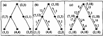
Consider Figure 1 (a). Each node stores a pair ( x, y), where x is a local constant and y is a sum initialized to x. To sum x at all nodes, we call CollectMessage from any root (b). SetMsgState consists of adding incoming numbers toy, and setting the message to a neighbor V as the sum of x and all incoming numbers except that from V. The sum can now be retrieved from the root. Next, we call DistributeMessage at the same root (c). The sum can now be retrieved from any node.

3 Probability propagation in JTs

Various methods for inference in BNs have been con­ structed [6, 1, 4, 8, 9, 2]. Several [4, 9, 2] use a junction tree ( JT) as mntime structure. We review how to con­ vert a BN into a JT and then consider two of them.

3.1 Conversion of a BN into a JT

A BN S is a triplet (N, D, P) where N is a set of variables, D is a DAG whose nodes are labeled by el­ ements of N, and P is a joint probability distribution

(jpd) over N. D encodes independence inN through d-separation [6], and hence P(N) = DxEN P(xj1r(x)), where 1r(x) is the parents of x in D.

Conversion of a BN starts with moralization. It con­ verts a DAG into an undirected graph by completing the parents o f each node and dropping direction of links. The result is called a moral graph. Then trian­ gulation (see Section 4) converts the moral graph into a chordal graph [7].

A JT over N is a tree where each node is labeled by a subset (called a cluster) of N and each link is labeled by the intersection (called a sepset) of its incident clus­ ters, such that the intersection of any two clusters is contained in every sepset on the path between them1.

A maximal complete set of nodes in a graph is called a clique. After the triangulation step, a JT for a BN is created with nodes labeled by cliques of the chordal graph. Such a JT exists iff the graph is chordal.

After a JT is created, distributions in the BN are as­ signed to the clusters. For each x E N, P(xj1r(x)) is assigned to a cluster containing x and 1r( x).

3.2 Shafer-Shenoy propagation

S-S propagation [9] is static, where each cluster holds a belief table over its variables, defined as the product of all distributions assigned to it. Hence the product of the belief tables in all clusters is the jpd.

During propagation, each message sent over a sepset is a belief table over the variables in the sepset. SetMs­ gState consists of multiplying the local table with in­ coming tables from other neighbors and marginalizing the product down to the corresponding sepset. For each cluster, after the propagation, the product of the local tables and all incoming tables is the marginal probability distribution over the variables of the clus­ ter.

3.3 Lazy propagation

Lazy propagation [5] is also static, where each cluster C holds the assigned distributions as a set rather than as a product. The belief table of C is defined the same as above but the product is not explicitly computed (hence the reduced space complexity over the S-S and HUGIN methods).

Each message sent over a sepset is a set of tables each of which is over a subset of the sepset. SetMsgState to a given neighbor consists of taking the union of local tables and incoming tables from other neighbors, and then marginalizing out each variable not in the sepset.

1 The property is a.lso known as running intersection.

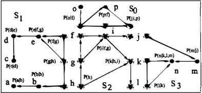
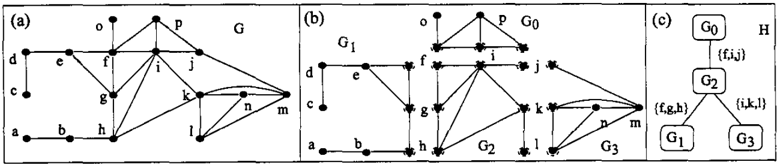
Figure 3: (a) G is the union of the graphs in (b) . (b) G is sectioned into four subgraphs. (c) A hypertree over G.

�

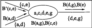
Figure 2: Message passing in lazy propagation.

Figure 2 illustrates lazy propagation. The cluster {a,c,d,e,g} has sepsets {a,d}, {c,e} and {d,e,g}. It has local tables {B(a,g), B(c, e)} and receives the tables B'(c,e) and B(a,d). It sends out B(d,g) == I:.B(a,d)B(a,g) and B(e) == LcB(c,e)B'(c,e).

4 Triangulation as tree propagation

We consider triangulating an undirected graph orga­ nized as a (hyper) tree.

Definition 1 Let G; == (N;, E;) (i == 0, . . . , n-1) be n graphs. The graph G == (U;N;, U;E;) is the union of G;s, denoted by G == U;G;.

If for each i and j, l;j == N; n Nj spans identical sub­ graphs in G; and Gj, then G is sectioned into G;s. l;j is the separator between G; and G j.

The graph in Figure 3 (a) is sectioned in (b) . Each node in a separator is highlighted by a dashed circle.

Definition 2 Let G == (N, E) be a connected graph sectioned into {G; == (N;, E;)}. Let the G;s be orga­ nized as a connected tree H where each node is labeled by a G; and each link is labeled by a separator such that for each i and j, N; n Ni is contained in each subgraph on the path between G; and Gj in H 2 . Then H is a hypertree over G. Each G; is a hypernode and each separator is a hyperlink.

Figure 3 (c) shows a hypertree H over G in (a) . Note that the above concepts are applicable to both directed and undirected graphs.

Definition 3 Let H be a hypertree over a graph G sectioned into { G;}. Let G' be a graph from a trian­ gulation of G such that each clique in G' is a subset of

2 Note the similarity to JTs.

some N;. Then the triangulation is constrained by H.

A node x in an undirected graph is eliminated by adding links such that all of its neighbors are pair­ wise linked and then removing x together with links incident to x. The added links are called fill-ins.

Theorem 4 ([7]) A graph is chordal iff all its nodes can be eliminated one by one without adding fill-ins.

Let a hypertree H over G be rooted at a given hyper­ node G;. An elimination order p of G is constrained by H if p consists of recursively eliminating nodes that are only contained in a single leaf hypernode of H.

Proposition 5 An elimination order of G con­ strained by a hypertree H over G produces a trian­ gulation of G constrained by H.

Triangulation constrained by H can be performed as a (dynamic) rooted collect propagation of fill-ins: Let G; be the child of Gj in H with separator I;j == N; n Nj. The message sent from G; to G j is a set of fill-ins over l;j. SetMsgState consists of the following:

Algorithm 1 (SetMsgState for propagating fill-ins) add to G; fill-ins received from each neighbor except G1; eliminate N; \ N1 and add fill-ins to G;; set message to G1 as all fill-ins over l;j obtained above;

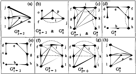
Suppose H is rooted at G1. For G1, SetMsgState is simplified ( Gj == null, Nj == ¢ and the last step is not applicable) . Figure 4 illustrates the collect propaga­ tion of fill-ins.

p 1

二

:�,

It can be shown that fill-ins sent during collect propa­ gation of fill-ins is independent of the elimination order used by SetMsgState in each hypernode and are deter­ mined uniquely by the chosen root. Hence if H has n hypernodes, potentially n different triangulations of G (assuming each local elimination is optimized without ties) can be obtained each from a collect propagation at a distinct root. To obtain then triangulations, how­ ever, we do not have to perform collect propagation n times. Instead, a full propagation in H is sufficient:

CollectMessage will be performed as above. Dis­ tributeMessage will be performed with the same SetMsgState (Algorithm 1). Finally, each non-root performs SetMsgState as if it is a root,

Figure 5 illustrates the full propagation with H in Fig­ ure 3. The root is G1. During CollectMessage, SetMs­ gState is first performed in Go and G�. Suppose the elimination order in G3 is (n, m ) . The fill-ins produced are { {j, k }, {j, /}} as shown in (a) with dashed links. The resultant chordal graph is labeled Gij_. 2· Ga sends the above fill-ins to G2. Similar operations then occur in Go (b) and G2 (c).

Since G1 is the root, it performs a simplified SetMs­ gState. After adding the fill-in {!, h}, the resultant graph Gi is chordal as shown in (d) . CollectMessage now terminates. DistributeMessage follows as shown in (e) to (g). Each non-root hypernode performs one more SetMsgState as if it is a root with the results shown in (b), (c) and (h). Note that in (h) , since the received fill-in is {j, k} and the elimination can be per­ formed in any order, G3 is simpler than G 3 _.2 .

5 Overview of MSBNs

An MSBN M is a collection of Bayesian subnets that together defines a BN [11, 10]. M represents proba­ bilistic dependence of a total universe partitioned into multiple subdomains each of which is represented by a subnet.

Just as the structure of a BN is a DAG, the structure of an MSBN is a multiply sectioned DAG (MSDAG) with a hypertree organization:

Definition 6 A hypertree MSDAG 1J = U D; 1 where each D; is a DAG, is a connected DAG such that {1} there exists a hypertree over 1), and {2} each hyper/ink d-separates {6] the two subtrees that it connects.

The second condition requires that nodes shared by two subnets form a d-sepset:

Definition 7 Let D; = (N;,E;) (i = 0,1) be two DAGs such that D = Do U D1 is a DAG. The in­ tersection I = No n N1 is a d-sepset for Do and D1 if for every x E I with its parents 7r( x) in D 1 either 1r(x) <; N0 or 7r(x) <; N1. Each x E I is called a d-sepnode.

This is established as follows:

Proposition 8 Let D; = (N;, E;) (i = 01 1) be two DAGs such that D = Do U D1 is a DAG. No \ N1 and N1 \ N0 are d-separated by I = No (l N1 iff I is a d-sepset.

It can be shown that the above definition of MSDAG is equivalent to the constructive definition in [11]. An MSBN is defined as follows:

Definition 9 An MSBN M is a triplet M = (N, 1J, 'P). N = U; N; is the total universe where each N; is a set of variables. 1) = U; D; (a hypertree MSDAG) is the structure where nodes of each DAG D; are labeled by elements of N;. Let x be a variable and 11'( x) be all parents of x in 1). For each x 1 exactly one of its occurrences {in a D; containing { x} U 7r( x)) is assigned P(x\1r(x))1 and each occurrence in other

√

DAGs is assigned a constant table. P = Il; Pn, is the jpd, where each Pn, is the product of the prob­ ability tables associated with nodes in D;. A triplet S; = (N;, D;, Pn.) is called a subnet of M.

An example MSBN is shown in Figure 6.

6 Compilation of MSBNs

So far, inference in MSBNs [11, 10] has been an exten­ sion to the HUG IN method [2]3, which works with one triangulation and one decomposition of messages for the entire propagation. As demonstrated in Section 4 and below, it is possible to let the triangulation and decomposition depend on the direction of messages. The resultant clusters can be smaller than obtained by the HUGIN method. Below we explore this idea for inference in MSBNs using the S-S and lazy propa­ gation.

6.1 Local structure for message/inference

First moralization is performed as a full dynamic prop­ agation on the hypertree. A message sent from a hy­ pernode to another consists of (moral) links over their d-sepset. During CollectMessage, SetMsgState con­ sists of the following: ( 1) For each hypernode, parents of each node in D; are completed and directions of links are dropped. (2) Moral links from each child hypernode are then added. (3) Set the message to the parent hypernode as the moral links over their d­ sepset. For DistributeMessage, SetMsgState consists of (2) and (3). Figure 3 (b) is the moralization of the MSBN in Figure 6.

Next triangulation is performed as in Section 4. Then we convert each Gi into a JT for local inference (as in Section 3.1) and convert each Gi'-tj into a junction forest (JF) for computing messages from subnet S; to Sj for inter-subnet belief propagation. We present the conversion of Gi-tj into a message JF below:

To see the need of multiple structures for each subnet, observe that Gi is generally more densely connected than Gi-t j . In Figure 5, the d-sepset is complete in Gi,

3The HUGIN propagation is dynamic whereas S-S as well as lazy propagation are static.

but incomplete in Gi .... 2. By using Gi-tj· the message from sl to s2 can be decomposed into two submes­ sages, one over {!, g} and the other over {g, h}. This results in a more compact message representation. For each Gi-+ i ' we organize its cliques into a set of JTs (a JF) so that each submessage can be obtained directly from one cluster of each JT. Without formally pre­ senting the general algorithm, we illustrate using the example in Figure 5.

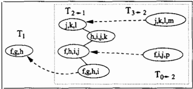
First, consider G3 .... 2· Since the d-sepset is complete (no opportunity for message decomposition) , we or­ ganize the cliques of G3 .... 2 into a JT Ta-t2 shown in Figure 7 ( 1). During inference, the message from Sa to s2 can then be obtained from the cluster {j' k' l' m}. Similarly, JTs To-t2, T2-tl and T2-to can be obtained.

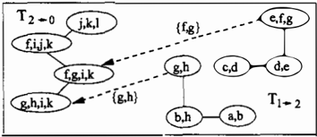
Next, consider G't .... 2· Since the d-sepset is incomplete (the message is decomposable) , we create a JF con­ sisting of two JTs as in (2). During inference, the submessage over {f, g} can be computed using the up­ per JT from the cluster { e,f, g }. The submessage over {g, h} can be obtained from the cluster {g, h} of the lower JT.

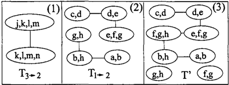
The JF is constructed as follows: For each clique in the subgraph of Gi .... 2 spanned by the d-sepset, create an isolated node labeled by the clique. Hence we obtain the two clusters at the bottom of (3). They are the candidate clusters from which the submessages will be obtained. We then complete the d-sepset in Gi .... 2 and create a JT out of it as shown in the top of (3). We split this JT into two and merge each with one of the candidate clusters as follows:

We delete the d-sepset cluster {f, g, h }, breaking the JT into two subtrees. For one subtree, the cluster {b, h} was adjacent to {f,g, h}. Since the candidate cluster {g, h} satisfies {g, h }n{b, h} = {f, g, h }n{b, h }, we connect {g, h} with {b, h}. For the other subtree, the cluster {e,f,g} was adjacent to {f,g, h}. Since the candidate cluster {f, g} is a subset of { e, f, g }, we remove the candidate cluster {!, g}. The resultant JF is the one in (2). Similarly, JF T2-t3 can be obtained.

Without confusion, we refer to message JFs and in­ ference JTs collectively as JFs. In the next section, we define a data structure to guide message passing between local JFs at adjacent subnets.

二

6.2 Linking message JFs and inference JTs

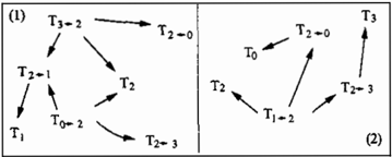
Inference in an MSBN can be performed as a full prop­ agation in the hypertree consisting of message passing among JFs (SetMsgState will be detailed later). When a message is to be sent from S; to Sj, it is computed using T;_.j. When Sj receives the message, it will be processed by T j and each Tj_.k (k =/; i). Figure 8 (1) illustrates directions of messages during collect propa­ gation with root sl' and (2) illustrates distribute prop­ agation.

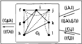
Figure Linkages between two message JFs. Figure 9 shows the two linkages from Tl-+2 to T2-+o used during distribute propagation. It reflects the fact that the d-sepset {!, g, h} can be decomposed into two independent subsets {f, g } and {g, h} conditioned on their intersection {g}. Each linkage (shown as a dashed arc) is labeled by the intersection of the two end clusters. We shall call the two clusters the hosts of the linkage. Once linkages are determined, the set of all JFs forms a linked junction forest (LJF).

6.3 Belief assignment

Next, we assign conditional probability tables (CPTs) in the MSBN to clusters in the LJF. For each JF of each subnet, the assignment is performed as follows: For each variable .r, if a CPT is associated with it, then assign the CPT to a cluster in the JF that contains .r and its parents.

The joint system belief of the LJF is then defined as B(.N) = fl; fl j fl k f3i,j,k, where i is the index of infer­ ence JTs, j is the index of clusters in a given J T, f3i,j denotes the set of CPTs assigned to the jth cluster in the ith JT, and f3i,j,k is the kth CPT in the set. It is easy to see that B(N) is identical to the jpd of the MSBN.

Since CPTs are assigned in the same way in inference JTs and message JFs, the belief of all JFs from the same subnet are identical.

Although each subnet is associated with multiple JFs, only one copy of each CPT needs to be physically stored. For each CPT, it suffices to store a poin ter at the assigned cluster in each JF.

7 Shafer-Shenoy propagation in LJF

We extend the S-S propagation (Section 3.2) for infer­ ence in a linked junction forest.

For each cluster in each JF of each subnet, a belief ta­ ble is created by multiplying the CPTs assigned to the cluster. Inference is performed as a full propagation over the hypertree during which messages are sen t be­ tween JFs in ad jacent subnets. When a message JF has multiple linkages to an ad jacent JF, the message consists of multiple submessages (otherwise the mes­ sage consists of a single submessage) each of which is sent across a distinct linkage. Each linkage is used for message passing in a unique direction.

Each submessage is prepared at a distinct JT in a mes­ sage JF. A local collect S-S propagation is started at the linkage host and the submessage is then obtained at the host. The propagation involves incoming link­ ages and their hosts in the ad jacent JFs, as illustrated in Figure 10.

Figure 10: To compute the submessage from T2-+1 to T1, T2-+1 is extended (dotted box) to include link­ age hosts {j, k , l , m } from T3-+2 and {!, i,j,p} from To-+ 2. The collect propagation starts at linkage host {f,g, h, i}.

Now we define SetMsgState for preparing the message from S; to Sj sen t by message J F T;-+j:

Algorithm 2 (SetMsgState for S-S propagation in LJF)

for each junction tree of Ti-tj start collect S-S propagation at the host of linkage to S1;

set submessage as marginal of host belief to the linkage;

To analyze the effect of the propagation, we define the belief tables associated with different identities in an LJF: For each cluster C with a local belief table (3 and incoming messages (3; ( i = 1, . . . ) , the belief table Be (C) is the product (3* f]; (3;. Note that the messages

include messages from sepsets as well as submessages from linkages. For each inference JT T over N, the be­ lief table BT(N) is the product BT(N) = IJ; Be, (C;), where i indexes clusters ofT. It can be shown that the extended S-S propagation is coherent.

After the extended S-S propagation in the LJF, a S-S propagation needs be performed at an inference JT to answer local queries. Note that the collect stage of the propagation should be performed on the extended JT to count the incoming messages from ad jacent message JFs. Also note that when evidence is available on a variable in a subnet, it should be entered to a relevant cluster in each JF of the subnet.

8 Lazy propagation in LJF

The extended S-S propagation can be directly modified into extended lazy propagation in LJFs as follows:

For each cluster in each JF of each subnet, its belief table is defined in the same way as the extended S­ S propagation, but multiplication of assigned CPTs is not performed explicitly. The S-S propagation per­ formed in each JF is replaced by lazy propagation (Sec­ tion 3.3). Each message over a sepset and each sub­ message over a linkage will in general be a set of belief tables over a subset of variables of the sepset/linkage without being multiplied together. Theorem 10 shows that the extended lazy propagation ensures coherent inference.

Theorem 10 After a full extended lazy propagation in an LJF, for each subnet S; over N;, its inference JT 11 satisfies BT, (N;) = I:.N"\N; Ilj BT; (Nj ) , where j indexes inference JTs.

As for normal BNs, the main advantage of lazy propagation is its decomposed representation of be­ lief tables/messages. The decomposition leads to re­ duced space complexity, which is particularly signifi­ cant when the problem domain is very large.

9 Conclusion

We presented how to construct a linked junction for­ est (LJF) from a multiply sectioned Bayesian network (MSBN), and how to extend Shafer-Shenoy and lazy propagation for inference in such an LJF. It is worth­ while to compare the new methods with earlier work on the construction of LJF and the HUG IN based in­ ference method [11, 10].

First of all, the new method constructs multiple JFs for each subnet, one for local inference and the oth­ ers for inter-subnet message computation. The previ­ ous method, on the other hand, creates a single JT at each subnet for both local inference and inter-subnet message computation. With the new method, since each message JF is dedicated to the computation of messages to a particular subnet, its structure is less constrained and is generally more sparse. With the previous method, a JT must function correctly at all conditions (send and absorb messages to/from each ad jacent subnet) and it is thus more constrained, re­ sulting in generally more densely connected JT struc­ tures.

Although we have extended the S-S and lazy propaga­ tions in the LJF constructed by the new method, they can be modified to perform in an LJF constructed by the previous method as well. Given what we have pre­ sented, the modification is straightforward. To the S-S propagation, the benefit of using the new construction is more compact belief representation and more effi­ cient inference computation due directly to the sparser JF structure. To lazy propagation, the benefit is that the sparser structures provide better guidance to the propagation. To see this, imagine that if an entire mes­ sage JF is a single cluster, the burden of finding an effective marginalization order for computing a mes­ sage will be placed entirely at runtime. Hence, each message JF in the new construction can be viewed as a concise recording of a set of effective marginalization orders ready for runtime exploitation. 4 On the other hand, the LJF by the previous method needs not to maintain multiple JFs at each subnet. Inter-subnet message computation and local inference computation can then be completed by just one propagation in the only JT at a subnet (instead of several propagations one at each JF) .

This observation suggests a tradeoff between using an LJF constructed by the new method and that by the previous method. One factor in making a choice is the relative sparseness of the LJF obtained by each method, which depends on the topology of the MSBN in question. Another factor in practice is the empha­ sis placed on simplicity in control (which translates to development time) and efficiency in runtime computa­ tion.

Secondly, the extended lazy propagation has much lower space complexity than the previous HUGIN based inference for MSBNs due to the factorized stor­ age of belief. With the lazy propagation, for each CPT in the MSBN, only one copy needs to be stored in the LJF. Hence the total number of independent param­ eters stored in the LJF is 46 for the example MSBN. If full CPTs are stored to save the on-line derivation,

4 A marginalization order specifies the order in which each variable is to be marginalized out. Two such orders are equally effective if their computational complexity are the same.

二

92 values should be stored. With the HUGIN based method, the total storage of all belief tables for all clusters in the sparsest LJF has a size of 140. As the MSBN grows in size and connectivity, the sizes of clus­ ters of the LJF grow. The belief storage per cluster in an LJF grows exponentially with the cluster size with the HUGIN based method, while with the extended lazy propagation it grows only linearly. Therefore, the extended lazy propagation will allow much larger MS­ BNs to be constructed and used than possible with the HUG IN based inference, given one's computational re­ source.

Acknowledgement

We thank the anonymous reviewers for helpful com­ ments. The support of Research Grant OGP0155425 to the first author from NSERC of Canada is acknowl­ edged.

References

1. M. Henrion. Propagating uncertainty in Bayesian net­ works by probabilistic logic sampling. In J .F. Lemmer and L.N. Kana!, editors, Uncertainty in Artificial In­ telligence 2, pages 149-163. Elsevier Science Publish­ ers, 1988.
2. F.V. Jensen, S.L. Lauritzen, and K.G. Olesen. Bayesian updating in causal probabilistic networks by local computations. Computational Statistics Quar­ terly, (4):269-282, 1990.
3. D. Koller and A. Pfeffer. Object-oriented Bayesian networks. In D. Geiger and P.P. Shenoy, editors, Proc. 19th Conf. on Uncertainty in Artificial Intelligence, pages 302-313, Providence, Rhode Island, 1997.
4. S.L. Lauritzen and D.J. Spiegelhalter. Local compu­ tation with probabilities on graphical structures and their application to expert systems. J. Royal Statisti­ cal Society, Series B, (50):157-244, 1988.
5. A.L. Madsen and F.V. Jensen. Lazy propagation in junction trees. In Proc. 14th Conf. on Uncertainty in Artificial Intelligence, 1998.
6. J. Pearl. Probabilistic Reasoning in Intelligent Sys­ tems: Networks of Plausible Inference. Morgan Kauf­ mann, 1988.
7. D.J. Rose, R.E. Tarjan, and G.S. Lueker. Algorith­ mic aspects of vertex elimination on graphs. SIAM J. Computing, 5:266--283, 1976.
8. R.D. Shachter, B. D'Ambrosio, and B.A. Del Favero. Symbolic probabilistic inference in belief networks. In Proc. 8th Nat/. Conf. on Artificial Intelligence, pages 126--131, 1990.
9. G. Shafer. Probabilistic Expert Systems. Society for Industrial and Applied Mathematics, Philadelphia, 1996.
10. Y. Xiang. A probabilistic framework for cooperative multi-agent distributed interpretation and optimiza­ tion of communication. Artificial Intelligence, 87(12):295-342, 1996.
11. Y. Xiang, D. Poole, and M. P. Beddoes. Multiply sectioned Bayesian networks and junction forests for large knowledge based systems. Computational Intel­ ligence, 9(2):171-220, 1993.