Information/Relevance Influence Diagrams

Ali Jenzarli

Department of Management The University of Tampa 401 West Kennedy Bvd. Box 15F Tampa, FL 33606-1490, USA (813) 253-3333,

Abstract

In this paper we extend the influence diagram (ID) representation for decisions under uncertainty. In the standard ID, arrows into a decision node are only infonnational; they do not represent constraints on what the decision maker can do. We can represent such constraints only indirectly, using arrows to the children of the decision and sometimes adding more variables to the influence diagram, thus making the ID more complicated. Users of influence diagrams often want to represent constraints by arrows into decision nodes. We represent constraints on decisions by allowing relevance arrows into decisions nodes. We call the resulting representation information/relevance influence diagrams (IRIDs). Infonnation/ relevance influence diagrams allow for direct representation and specification of constrained decisions. We use a combination of stochastic dynamic programming and Gibbs sampling to solve IRIDs. This method is especially useful when exact methods for solving IDs fail.

Key Words: Decision analysis, influence diagrams, asymmetric decision problems, stochastic dynamic programming, Markov chain Monte Carlo, Gibbs sampling.

1 INTRODUCTION

In this paper we introduce a variation on influence diagrams that allows the use of arrows into decision nodes to represent constraints as well as information. We call this new representation an Information I Relevance Influence Diagram (IRID). In an IRID, we model a decision variable that is constrained by other variables by drawing relevance arrows from the other variables to the decision variable. But we also still allow purely infonnational arrows into decision nodes.

Information/relevance influence diagrams allow for direct representation and specification of constrained decisions. This representation is a partial solution to the broader a [email protected]

problem of representing and solving asymmetric decision problems. Asymmetry in decision problems occurs when some values of decision and/or chance variables are not allowed given certain values of their predecessors. Recent works by Smith et al. (1993), Shenoy (1993) and all the references therein offer a more complete treatment of this problem. However, none of them provide a direct and explicit representation of asymmetries concerning decision variables.

The advantage of our representation lies in the solution method we use to evaluate !RIDs. This method is a combination of stochastic dynamic programming and Gibbs sampling, an iterative Markov chain Monte Carlo algorithm (Jenzarli, 1995). This method allows us to model asymmetries concerning chance variables by using zero-one conditionals. Our solution method is especially useful when exact methods for solving influence diagrams fail.

In this paper we assume that the reader is already familiar with directed acyclic graphs (DAGs), and belief networks (Pearl, 1988). Briefly, we defme a BN as a DAG in which nodes represent variables, together with a specification for each variable of a conditional probability distribution for that variable given its parents. (If there are no parents, this is a marginal probability distribution for the variable.) It is assumed that the joint probability distribution of the variables is the product of these conditional probability distributions.

We also assume that the reader is already familiar with Markov chain Monte Carlo (Hastings, 1970) and Gibbs sampling (Geman and Geman, 1984; and Gelfand and Smith, 1990).

We organize this paper as follows. In Section 2 we review influence diagrams (IDs) and their properties. In Section 3 we describe solutions algorithms for IDs. In Section 4 we describe infonnation/relevance influence diagrams. In Section 5 we adapt the Gibbs sampling algorithm of Jenzarli (1995) to !RIDs and illustrate with an example.

2 INFLUENCE DIAGRAMS

In this section we review influence diagrams (IDs) and their properties. We describe the assumptions on which the ID decision model is based. And, we conclude with a note on randomization. We use a numerical example to illusttate ideas and concepts where appropriate.

Let us begin by recalling the standard definition of an influence diagram.

Definition 1. An influence diagram (ID) is a DAG with variables as nodes, together with a specification for only some of the variables of conditionals given their parents. We call those variables with conditionals chance variables, and those without decision variables. For each chance variable, we specify a set of possible values. For each decision variable, we specify a set of admissible values that we call decision alternatives. An ID has a special chance node that is a sink and that is a deterministic function of its parents. We call this node the value node. Arrows into chance nodes are called relevance arrows while arrows into decision nodes are called informational arrows.

Consider the oil wildcatter's problem adapted from Raiffa (1968). The wildcatter has to decide whether to drill or not drill. This decision is represented by the decision variable D whose values are d (drill) and nd (not drill). The values d and nd are decision alternatives. The wildcatter is uncertain about the amount of oil in the well. The amount of oil in the well is represented by the chance variable 0, whose possible values are w (wet) and y (dry). The cost of drilling is $950,000, and the estimated revenue from drilling a wet well is $2,000,000. Table 1 shows the wildcatter's net monetary payoffs and his subjective probabilities for 0.

d obl Table 1. Pavoff table for the wil catter s pr em

D
State		d (drill)	nd (not drill)	Probability of State
0	y (dry)	-$950,000	0	0.4
	w (wet)	$1050000	$0	0.6

More information about the amount of oil in the well can be obtained by conducting one of two seismic tests; test1 is standard and relatively affordable, while test2 is advanced and more costly. The seismic testing decision is represented by the decision variable T, whose values are t1 (test1), t2 (test2) and nt (no test). The seismic test result is represented by the chance variable R, whose values are o (open structure), supporting a dry well, c (closed structure), supporting a wet well, and or (no result), indicating that no seismic test has been performed. Finally, the payoff function is represented by the value node V, which is a function of 0, T and D.

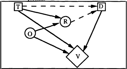
Figure 1 shows an ID for the oil wildcatter's problem, where chance variables are shown as circles, decision variables as rectangles, and the value node as a diamond.

Chance variables in an ID are interpreted just as they are in a BN. The conditional probability

Table 2. Conditional probability distribution of R given T and O

P ( X=x j X1 =x1, X2 =x2, ... , ?' t =xt } . (1) that we specify for a chance vartable X mdtcates our belief that X will take the value x when its parents, the X i , take the values X i . For the sake of generality, we will not rule out the possibility that the values of the conditional probability are unaffected as we change some of the X i . By drawing arrows to X from all the X i we signal that we think X depends on them all, and that we expect to specify values for (1) that do depend on them all. But if assessment of the probabilities follows the construction of the DAG, this expectation may fail to be fulfilled. In Figure 1 the chance variable R depends on the values of the decision variable T and the chance variable 0. The conditional probability distribution of R given T and 0 is shown in Table 2. Notice that the conditional probability of R given T = nt and 0 remains unchanged whether 0 = wor O= y.

		R
T	0	0	c	m
t1	w	0.2	0.8	0
t1	y	0.9	0.1	0
t2	w	0.05	0.95	0
t2	y	0.95	0.05	0
It	w	0	0	1
It		0	0	1

:1_

The decision maker can be asked to supply in advance a policy for the decision at each decision v � ble . t. . This policy usually takes the form of a s p ectficatton of a decision alternative for each configuration of the parents of the decision variable. For example, in Figure 1, when the oil wildcatter must decide whether to drill or not drill, he does so knowing his earlier choice at the decision variable T as well as the value of the chance variable R.

The result of such a policy can be interpreted as a conditional for Ji given its parents. This conditional gives only probabilities of zero and one:

where ()(x1, ··· ,xk) is the decision alternative that the decision maker deterministically chooses when he or she observes the values x1, ... ,xk of the parents. For example, in Figure 1, the wildcatter may supply a policy where he would use test2, i.e., T=t2, and drill only if T=t2 andR = c.

Notice that by supplying in advance conditionals for the decision variables, the decision maker turns the ID into a BN; he or she now has conditionals for all the variables given their parents.

In general, a chance node X in a BN or ID is called deterministic if its conditional is of the type (2), where a is replaced by X, d is replaced by x and ()(x1, ... ,xk) is replaced by f(x1, ... ,xt), f being the deterministic function that gives a value for X for every configuration x1, ... ,xk of the parents. We assume that an ID has exactly one sink, which is a deterministic chance node and which has real numbers for its values. The decision maker's purpose is to choose conditionals for the decision variables so as to maximize or minimize (optimize) the expectation of this node, which is called the value node and designated by V.

The decision maker may, if he or she wants, adopt a policy that makes the conditional for a decision variable depend on only some or none of its parents. For example, the wildcatter may adopt a policy that makes his conditional for whether to drill or not drill based only on the value of R, but not on the value ofT. In some cases, we can tell from the structure of the graph (without numerical calculations based on the conditionals for the chance nodes) that the best policy based on only some parents will do as well as the best policy based on them all. If some parents are omitted, then the corresponding arrows can be omitted; the graph with these arrows omitted will still be an ID, and once the decision maker has specified all the conditionals, it will be a BN. In general, description and computation in a BN or ID is easier with fewer arrows, so the decision maker would like to omit as many arrows as possible, but he or she may have to make his or her policy depend on all or most of the decision variables' parents in order to optimize the expectation of the value node. Thus the decision maker's objective is to make the policy depend on as few of the parents as possible while still optimizing the expectation of the value node.

Recall that the arrows into chance nodes are called relevance arrows and arrows into decision nodes are called informational arrows. Informational arrows indicate that the decision maker has certain information, not that he or she must use it. The relevance arrows will all remain in the BN that the decision maker constructs with his or her choice of conditionals for the decision variables, but the decision maker essentially omits informational arrows when he or she chooses a conditional that does not depend on the nodes from which these arrows come.

Following Clemen (1991), we distinguish between informational arrows and relevance arrows by representing the former with dashed arrows while still using solid arrows to represent the latter. Notice that decision variables are treated just like chance variables when they are parents. The difference between an informational and a relevance arrow depends on the kind of variable the arrow points to, not on the kinds of variables it comes from.

We follow Howard and Matheson (1981) and most of the ID literature in making two additional assumptions:

1. The decisions are all made by a single decision maker who remembers his or her previous decisions. This assumption is represented by the existence of a path in the DAG consisting only of all the decision variables. In other words, the decision variables are ordered, say al,a2, ... ,ak, so that there is an arrow from ai to ai+t· for i = 1, 2, ... , k-1. We summarize this by saying that the decision variables are completely ordered by the DAG.
2. The decision maker does not forget any previous information as he or she progresses through the decisions. This assumption is represented by the existence of an arrow from X to a i whenever there is an arrow from X to ai and i<j. In other words, each decision node inherits the parents of preceding decision nodes. This is called the no-forgetting assumption. Notice that a decision variable need not inherit the parents of chance variables that precede it. In Figure 1, for example, there is no arrow from 0 to D.

We conclude this section with a note on randomization that we include for completeness and that the reader may omit without loss of continuity. Recall that the decision maker can be asked to supply in advance a policy for the decision at each decision variable a . As we discussed above this policy can take the form of a specification of a decision alternative for each configuration of the parents of the decision variable. This policy can also take the form of a probability distribution over the decision alternatives for each configuration of the parents of the decision variable. For example, in Figure 1, the wildcatter has the option of choosing a probability distribution over the decision alternatives of whether to drill or not drill. In this case a probability distribution must be specified for each configuration of D's parents. For instance, he may decide to drill with probability 113 given T=tl and R=o, with probability 112 given T=tl and R=c, with probability 1/5 given T=t2 and R=o, with probability 9/10 given T=t2 and R=c, and with probability 114 given T=nt and R=nr.

The result of such a policy can be interpreted as a conditional for a given its parents. Again, the decision maker has conditionals for all the variables given their parents, and the ID becomes a BN. The decision maker's objective is still to make the policy depend on as few of the parents as possible while optimizing the expectation of the value node.

However, in optimizing the expectation of the value node, there is no advantage to randomization because of the convexity of the set of probability distributions that can be attained (von Neumann and Morgenstern, 1953). I ndeed, when we look at bow the expectation of the value node V is affected by varying the conditional for a particular decision node .d -futing for the moment conditionals for the other decision variables-we see that this expectation is an average of the expectations for V that would be obtained by fixed decision functions for .d . Such an average cannot be better than the best of the expectations being averaged (Dantzig, 1951). So instead of using conditionals for decision alternatives, researchers have traditionally used decision functions (Howard and Matheson, 1981).

3 SOLVING INFLUENCE DIAGRAMS

Solution algorithms for IDs can all be described as elaborations of various forms of the principle of optimality in stochastic dynamic programming, which allows us to fmd the decision functions in problems of this type sequentially (Bellman and Dreyfus, 1962).

In its standard form, the principle of optimality in stochastic dynamic programming applies when we want to maximize or minimize the expectation of a real-valued variable V whose joint distribution with k+ 1 other variables r 0, r 1, ... , r It (which may each be vectors of variables) depends in a stagewise manner on k parameters (which also may be single numbers, vectors or functions) 51, ... , a lt. More precisely, we assume that we can factor the joint probability for r 0, r 1, ... , r 1c and v in the form

where the factors are conditional probabilities. We must also assume that it is com � utationally feasible to compute from

for each value of alt and each configuration of values of r 0u ... ur Jt-1, or at least to find for each configuration ('Yo····· 'Y�c-d of r 0u ... ur �c-1 the value of S�c that op timizes

Finally, we must assume (this is crucial) that we can fmd a single value of ale that optimizes (4) for all ('Yo·····'Y�c-tl· Since the distribution of r0u ... u r �c_1 does not depend on alt. we have

Therefore, this optimizing value of Sit will also optimize the unconditional expectation E61 . .. A (V) for any choice of ( 5 1, . . . ,5 � _1). And therefore, it can be extended to a choice of t51, . . . ,SJt) to optimize this unconditional expectation.

Suppose we fix this optimal value of St eliminating it from our notation, and reducing (3) to

From this point, we proceed in either of two ways. We can sum or integrate r It out of the expectation. Or we can inco rporate r t as part of r t-1 ·

The first option, summing or integrating F out, means reducing (5) to

where

Once again, we assume that we can choose a single value of 5�c_1 so as to optimize simultaneously

for all ( 'Y 0, . . . , 'Y It 2 } . Then, as before, the choice of o k-1 can be extended to a choice of (S1, ... ,Sit_1) to optimize the unconditional expectation

So we may also fiX this optimal value of o1H, and reduce the problem further. We can continue in this way, choosing the oi sequentially, provided that the successive simultaneous optimizations like those in (4), (6), etc. are possible.

The second option means setting rJ.:_1 = r Jt -1 u r It· and reducing (5) to

where

Again, if we can choose 5t_1 to optimize simultaneously (6) for all (y0, ··· , y lt _ 2), and so on, we can proceed to choose the 8i sequentially.

This standard version of stochastic dynamic programming is not quite adequate for the case of influence diagrams. The reason is that although these diagrams involve

factorizations that can be written in the form (3), the factors are not necessarily conditional probabilities.

The standard version of stochastic dynamic programming can be modified to fit influence diagrams, but there bas been a considerable variety of opinion about bow to do this. The oldest sequential solution algorithm for influence diagrams, the Olmsted-Shacbter reduction algorithm (Olmsted, 1983; Shachter, 1986) goes considerably beyond stochastic dynamic programming, in order to maintain a representation of the influence diagram form as the algorithm proceeds. More recent algorithms, including the valuation network algorithm of Sbenoy (1992 and 1993) and the potential influence diagram algorithm of Ndilikilikesba (1992), stay closer to stochastic dynamic programming.

The simulation algorithm we will describe in Section 5, does not fit exactly into either Sbenoy's or Ndilikilikesba's framework, primarily because their algorithms integrate r k out, while our algorithm follows the second option described above, that of absorbing r k into h11 · We could elaborate one of their frameworks in orderttb make our algorithm fit, but it will be simpler for us to deal directly with the necessary modification in the standard form of stochastic dynamic prog ramm ing that we have just described.

Here is the modification that we require. Let us assume that the joint probability for r 0' r 1 ' ... ' r k and v is proportional to a factorization of the following form

Here we do � assume that the factors are conditional probabilities. But we .W assume that the 8i are functions; and we assume, as the notation indicates, that for fixed values of ro.rt>:···r k-1 · the factor b ll t l ro . ..r t -1.)' regarded as a function of r k and V, depends on 8k onry through the value Sk assigns to those values of r 0, r 1, ... , r k-1 . This assumption, as we will see implies that the simultaneous optimizations at each step are possible.

Notice first that the factorization (7) implies that

for ftxed values of r 0, r1 , ... , r k-1, is at least proportional to the conditional probability distribution for r k and V given these values of r 0 , r 1, ... , r t-1 . To see this, recall that a conditional probability distribution is always proportional to the corresponding joint probability distribution. Thus

where A. is constant with respect to r k and V. (The other variables are thought of as ftxed.) We usually write (8) with a symbol of proportionality:

Since only the last factor of (7) involves r k or V, (8) implies that

Again, this proportionality is to be interpreted by taking both sides as functions of r k and V only, with the other variables ftxed; we are able to omit the other factors only because they, as functions of the other variables, are also fixed and hence can be absorbed into the constant of proportionality.

Whenever a function is proportional to a probability distribution (or probability conditional), it contains all the information needed to find that conditional because the constant of proportionality is simply what is needed to make the function sum (or integrate) to one. Thus

bas, in particular, all the information needed to determine the conditional e � ctation V given ('Yo ... , 'Y �-1),

We can choose the value of 8t(y0, ... , 'Yt-1) to optimize this expectation, and by doing this for each set of values (ro .... , yk-1), we will have chosen a function sk that simultaneously optimizes (9) for all ( 'Y 0, ··· , 'Y k-1) .

Once this choice of Sk bas been carried out, we can proceed, as before : abso � bing h 11 t ( r 0 . . . ..rt,,) into h11 t _,(r ,o . .... r t -l ) , ftrst mtegrating 'Yt out tf we wtsh to do so. Thts means replacing the factor in the second line of (7) with a factor where

(1) r�t_1 = r k-1 u r k,

(2) �k, which is in r k, is now interpreted as a chance node , and

where s; is the optimal decision function and h � is the zero-one conditional representing s;. t

In order to fit influence diagrams into this version of stochastic dynamic programming, we write r i for the set of variables consisting of �i together with the chance variables observed by the decision maker between �i and

ai+1· for i = 1, ... , k-1, we write ro for the chance variables observed before a1 and r t for the set of variables consisting of lit together with the chance variables (other than V) observed after lit (or never), and we write 8i for the decision function for ai. Then we set h 0(r 0) equal to the product of conditionals for the chance variables in r 0· For i = 1, ... , k-1, we set h11 (rdr 0, .. . , r i _ 1 ) equal to the product of conditionals fo i the chance variables in r i, times the conditional corresponding to the decision function 8i (recall Formula (2)). And we similarly set h11 (r t· vir 0, ... , r t-1) equal to the product of the conditionals f or all varia b les in rt u{V}. Since h11 (rt,VIr0, ... , rt_t) depends on at only through its val � 8t(r o ..... r t-1). this puts us in the framework just described.

In the computational theory of Section 5 we will use Gibbs sampling to implement the method just described.

4 INFORMA TIONIRELEVANCE INFLUENCE DIAGRAMS

In the standard influence diagram, arrows into a decision node are only informational; they do not represent constraints on what the decision maker can do. We can represent such constraints only indirectly, using arrows to the children of the decision.

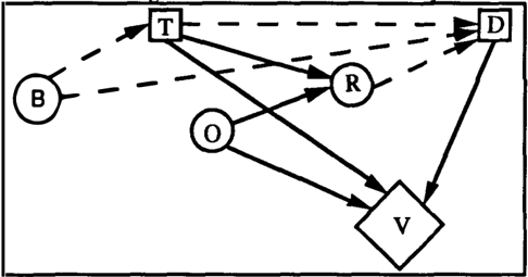
Users of influence diagrams often want to represent constraints by arrows into decision nodes. For example, a user might draw Figure 2 in an attempt to represent the fact that the budget, B, constrains the options for testing and drilling. However, Figure 2 cannot represent such constraints because the dashed arrows are only informational, and the figure does not show B having any relevance to any chance variables. If Figure 2 is interpreted as a standard influence diagram, then variable B will have absolutely no effect on the optimal decision functions; they are the same with or without it

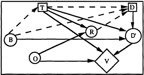
In order to represent a budget constraint using the standard ID rep resen tation, we would have to complicate the diagram of Figure 2 in some way. One way is represented in Figure 3. Here D' is a deterministic chance node representing whether drilling actually takes place as a function of the budget and the decision maker's decisions. For example, if the possible budget amounts are $1M (million) or $2M (million), the tests costs are $50,000 for testl and $100,000 for test2, and the cost of drilling is $950,000, then the decision maker cannot drill if B =$1M and T = t2. Using Figure 3, we can represent this by making D' (whether the drilling really takes place) a deterministic function of B, T and D as follows:

1. D' = f(B =$2M, T = nt, D =d)= yes
2. {2) D' = f(B = $2M, T = nt, D = nd) = no
3. D' = f(B =$2M, T = tl, D =d)= yes
4. D' = f(B =$2M, T = tl, D = nd) =no
5. D' = f(B = $2M, T = t2, D = d) = yes
6. D' = f(B = $2M, T = t2, D = nd) =no
7. D' = f(B = $1M, T = nt, D = nd) = no
8. D' = f(B =$1M, T=nt, D= d)= yes
9. D' = f(B =$1M, T= tl, D= d)= yes
10. D'=f(B=$1M, T=t1,D=nd)=no
11. D' = f(B =$1M, T= t2, D= d) =no
12. D' = f(B = $1M, T = t2, D = nd) =no

As line {11) indicates, the decision maker's purported decision to drill does not result in drilling if he or she does not have the money.

The complexity of Figure 3 is obviously undesirable. This suggests that we go beyond the standard ID definitions and allow relevance arrows into decision nodes. Such arrows would indicate both that the decision maker knows the value of the variables from which these arrows emanate when he or she makes the decision, and also that the variables constrain the decision.

This suggests the following formal definitions.

Definition 3. An information/relevance influence diagram (IRID) is a DAG with variables as nodes, some of which are called chance variables and some of which are called decision variables, together with

Definition l. A constraint on a variable X given a set of variables X 1 .... , X k is a mapping Cx from the frame of X 1 , ... , X k to subsets of the frame of X. (In other words, for each configuration x 1 , ... , X k of X 1 , ... , X k , we specify a set Cx(x 1 , ... , X k ) of permitted values for X.)

1. a specification, for each chance node X, of a conditional for X given its parents, and
2. a specification, for each decision node a, of a constraint for a given a subset S a of its parents.

We divide the arrows into relevance arrows, which are solid, and informational arrows, which are dashed, as follows:

1. all arrows into a chance node X are relevance arrows,
2. arrows into a decision node !:t. from parents in Sa are relevance arrows, and
3. all other arrows into !:t. are inf orma tional arrows.

Here, as in the case of IDs, we assume that there is a value node: a deterministic chance node which is a sink and is real-valued.

We interpret IRIDs by assuming that when the decision maker makes decision !:t., he or she has observed all the parents of !:t.., including both those from which there are informational arrows and those from which there are relevance arrows. The relevance arrows indicate information for the decision maker as well as constraints on the decision.

We assume complete ordering and no-forgetting for decision variables:

1. There is a path in the DAG consisting only of decision variables. (Some or all of the arrows on this path may be relevance arrows.)
2. If the decision variables, 1:t. 1 , ... , l:t. k , are ordered by the path that joins them and there is an arrow from X to �. then there is an arrow from X to l:t. j , for all i<j. (Again, there is no restriction on whether these arrows are relevance or informational arrows, or whether one is a relevance arrow and the other is an informational arrow.)

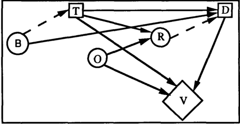
Figure 4 shows how the budget constraint for the wildcatter problem can be represented in an IRID. We start with the ID of Figure 2. We create a chance node for the variable B. Then we draw an informational arrow from B to T, a relevance arrow from B to D, and we replace the informational arrow from T to D by a relevance arrow.

Fi ure 4. IRID for the oil wildcatter's

For the diagram of Figure 4 we specify the following conditionals and constraints:

P(B = $1M)=0.50=1 - P(B =$2M)

P(O = w) =0.60=1 - P(O = y)

P(R=o I O=w, T=t1) =0.20=1-P(R=e I O=w, T=tl)

P(R=o I O=w, T=t2) =0.05=1-P(R=e I O=w, T = t2) P(R=o I O=y, T=t1)=0.90=1-P(R=e I O=y, T=t1) P(R=o I O=y, T=t2)=0.90=1-P(R=e I O=y, T=t2) P(R = nr I 0, T = nt) = 1.0 V(O = w, T = nt. D = nd) = -$2,000,000 V(O = y, T = nt. D = nd) = $0 V(O = w, T = nt. D = d) = $1,050,000 V(O = y, T = nt. D = d) = -$950,000 V(O = w, T = t1, D = nd) = -$2,050,000 V(O = y, T = t1, D = nd) = -$50,000 V(O = w, T = t1, D = d) = $1,000,000 V(O = y, T = t1, D = d) = -$1,000,000 V(O = w, T = t2, D = nd) = -$2,100,000 V(O = y, T = t2, D = nd) = -$100,000 V(O = w, T = t2, D = d) = $950,000 V(O = y, T = t2, D = d) = -$1,050,000 Co(B =$1M, T = nt) = { d,nd } Co(B =$1M, T = t1) = { d,nd } Co(B = $1M, T = t2) = { nd } Co(B =$2M, T = nt) = { d, nd } Co(B =$2M, T = t1) = { d,nd } Co(B =$2M, T = t2) = { d, nd }

Notice that the theory of stochastic dynamic progr amm ing that applies to IDs also applies to IRIDs; it is simply necessary that each step in the optimization respect the constraints.

5 SOLVING IRIDS

We begin this section with a review of the simulation algorithm for solving IDs given in Jenzarli (1995). Then we adopt the algorithm to IRIDs. Finally, we apply the adapted algorithm to the IRID of the oil wildcatter problem.

Jenzarli (1995) shows how to use Gibbs sampling (Geman and Geman, 1984; and Gelfand and Smith, 1990), an iterative Markov chain Monte Carlo algorithm (Hastings, 1970), to implement stochastic dynamic programming for an influence diagram. For an ID with k decision variables !:t.1 ····· !:t.k and sets r O ··· · ·r k as described in Section 3, we give a brief summary of the simulation algorithm.

Our task is to find the decision function lit. This means finding, for each configuration ( y 0, y 1, ... , y kt ) of r0u ... ur�c._1, the value dt of the decision !:t.k that optimizes

Ed (vir o = 'Yo·r1 = 'Y1·····r t-1 = 'Yt-1)· (10) (Notice that we write d k in the place of S�r. as a subscript on the expectation operator; this is because the expectation for the configuration (y0, y1, . . . , 'Yt-1) of the predecessors depends only on the value dk that sk assigns to this configuration.) To this end, we simply compute (10) for all dt and choose the dt that gives the optimal (largest or smallest depending on whether we are maximizing or minimizing) result.

To compute (10) for a particular dt, we recall that the conditional joint disttibution of r t u {V} is proportional to h d k ( rt,V I r o =r0 .... ,rt_1 =rt-d· which is simply the product of the conditionals for r t u {V}. We now give the steps involved in the computation of (10).

1. Delete all barren nodes form the ID (Shachter, 1986).
2. Draw the ID according to the information partitioning implied by r0, ··· ,rt and omit inf orma tional arrows.
3. Omit any variables from r t that are not connected with V in the subgraph of this moral graph determined by r t u {V}. The result is rt.
4. Form the moral graph.
5. Omit any variables not in rt u {V} that are not neighbors of rt in the moral graph of Step 4. The variables that remain are the variables on which .dt depends that are not in rt u {V}.
6. The factors remaining in the joint disttibution are those in which the variables remaining in rt are either parents or children.
7. ( 6) Draw the directed sub graph determined by all the variables that remain.
8. Now that the factors are identified , we do Gibbs sampling with these factors to simulate the joint distribution of rt \ { .& t, V}. First, we fix the variables on which .dt depends that are not in rt u {V}. Then, for the configuration of rt \ {.&t, V} obtained at each step of the Gibbs sampling, we compute V. This gives a sequence of values for V simulating a random sample from its conditional disttibution, from which we may compute its conditional expectation.
9. When we move on to the next step of the stochastic dynamic program, we use the second of the two options discussed in Section 3. In other words, we absorb r t into r t-1· and we include the conditionals from r t in the new factorization of h11 · In order to avoid zero probabilities that would lii1terfere with the Gibbs sampling, we do not include the conditional for .dt corresponding to the decision function we have just found for .&t. Instead, we substitute this decision function in all the conditionals in which .& t appeared as a parent, thus eliminating .dt from the graph and producing arrows from the variables on which .dt depends to the variables for which it was a parent.

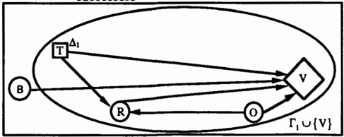
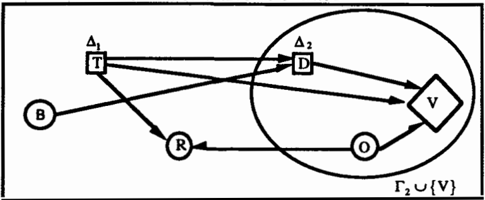
The algorithm we have just described for IDs also works for IRIDs. The only point to note is that the relevance arrows into .dt must be included in the graph from which the moral graph is formed. We now apply the algorithm to the IRID of the oil wildcatter problem. Figure 5 shows the IRID of the oil wildcatter problem with informational arrows omitted, where

2

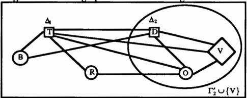
We now form the moral graph as shown in Figure 6. Notice that according to Step 4 of the algorithm, r 2 = r2 . Also, all variables not in r2 u {V} are neighbors of r; in the moral graph of Figure 6. This means that the variables on which D depends are T, R, and B. Thus the factors to consider in the joint disttibution are those in which D and 0 are either parents or children. These factors on which we do Gibbs sampling are:

P{R= ·IT= ·.O)P(D= ·IT= ·,B = ·)P{O) , where · means that the value of the variable in question is fixed.

Next we do Gibbs sampling with these factors to simulate the posterior disttibution of 0. First, we fix the variables on which D depends, i.e., T, R, and B. Then for every value of 0, we compute V. This gives a sequence of values for V simulating a random sample from its conditional disttibution, from which we may compute its conditional expectation. We perform this step for every value of D, and we choose the value of D that corresponds to the maximum conditional expectation of V.

When we move on to the next step of the stochastic dynamic program, we absorb r 2 into r 1 as described in Step 9 of the algorithm. Then we eliminate D from the graph, thus producing arrows from T, R, and B to V. The resulting graph is shown in Figure 7.

successors

Figure 7. DAG with D absorbed into its direct

Finally, we include the conditionals from r 2 in the new factorization of b6 · In order to avoid zero probabilities that would interf � with the Gibbs sampling, we do not include the conditional for D corresponding to the decision function we bave just found for D. Instead, we substitute this decision function in all the conditionals in which D appeared as a parent.

Acknowledgments

This work was partially supported by the National Science Foundation under grants IRI-8902444 and SES-9213558, and by a grant from the General Research Fund at the University of Kansas, grant 3605-XX-0038. Other partial support came from a Globe Project grant at the University of Tampa. I am grateful for comments from my mentors Glenn Shafer and Prakash Shenoy. I am especially grateful for the help and encouragement I received from Glenn Shafer.

References

Bellman, R. and Dreyfus, S. (1962) Applied Dynamic Programming, Princeton University Press, Princeton, NJ.

Clemen, R.T. (1991) Making Hard Decisions, Duxbury Press, Belmont, California.

Gelfand, A. E. and Smith, A. F. M. (1990) Sampling­ based approaches to calculating marginal densities, Journal of the American Statistical Association, 85(410), 398-409.

Geman, S. and Geman, D. (1984) Stochastic relaxation, Gibbs distributions, and the Bayesian restoration of images, IEEE Transactions on Pattern Analysis and Machine Intelligence, PAMI-6, 721-741.

Hastings, W. K. (1970) Monte Carlo sampling methods using Markov chains and their applications, Biometrika, 57(1), 97-109.

Howard, R. A. and Matheson, J. E. (1981) Influence diagrams. In R. A. Howard and J. E. Matheson (eds.), Readings on the principles and Applications of Decision Analysis, vol. 2, Strategic Decisions group, Menlo Park, CA, 1984,719-762.

Jensen, F. V., Lauritzen, S. L., and Olesen, K. G. (1990) Bayesian updating in causal probabilistic networks by local computations, Computational Statistics Quanerly 4, 269-282.

Jenzarli, A. (1995) Solving Influence Diagrams Using Gibbs Sampling, Proceedings of the Fifth International Workshop on Artificial Intelligence and Statistics, 278284.

Ndilikilikesba, P. ( 1992) Potential influence diagrams, Working Paper No. 235, School of Business, University of Kansas, Lawrence, Kansas.

Olmsted, S. M. (1983) On representing and solving decision problems, Ph.D. thesis, Department of Engineering-Economic Systems, Stanford University, Stanford, CA.

Pearl, J. (1988) Probabilistic Reasoning in Intelligent Systems: Networks of Plausible Inference, Morgan Kaufman, San Mateo, CA.

Raiffa, H. (1968) Decision Analysis, Addison-Wesley, Reading, MA.

Sbacbter, R. D. (1986) Evaluating influence diagrams, Operations Research, 34(6), 871-882.

Shenoy, P. P. (1992) Valuation-based systems for Bayesian decision analysis, Operations Research, 40(3), 463-484.

Shenoy, P. P. (1993) A new method for representing and solving Bayesian decision problems, in D. J. Hand (ed.), Artificial Intelligence Frontiers in Statistics: AI and Statistics III, 119-138, Chapman & Hall, London.

Shenoy, P. P. (1993) Valuation Network Representation and Solution of Asymmetric Decision Problems, Working Paper No. 246, School of Business, University of Kansas, Lawrence, Kansas.

Smith, J. E., Holtzman, S. and Matheson, J. E. (1993) Structuring Conditional Relationships in Influence Diagrams, Operations Research, 41(2), 280-297.