Contents
1301.7398
Lazy Propagation in Junction Trees
Anders L. Madsen
Department of Computer Science Aalborg University Denmark [email protected]
Abstract
The efficiency of algorithms using sec ondary structures for probabilistic inference in Bayesian networks can be improved by ex ploiting independence relations induced by evidence and the direction of the links in the original network. In this paper we present an algorithm that on-line exploits indepen dence relations induced by evidence and the direction of the links in the original network to reduce both time and space costs. In stead of multiplying the conditional proba bility distributions for the various cliques, we determine on-line which potentials to multi ply when a message is to be produced. The performance improvement of the algorithm is emphasized through empirical evaluations in volving large real world Bayesian networks, and we compare the method with the HUGIN and Shafer-Shenoy inference algorithms.
1 Introduction
It has for a long time been a puzzle why "stan dard" inference algorithms for Bayesian networks did not really use the direction of the links in the network. By "standard" we mean the Lauritzen Spiegelhalter [Lauritzen and Spiegelhalter, 1988], the Shafer-Shenoy [Shafer and Shenoy, 1990], and the HUGIN [Jensen et al., 1990] algorithms and the vari ous variations over these algorithms ( [Shachter, 1990] and [Jensen, 1995]). These algorithms build a sec ondary structure (a junction tree or a join tree) by triangulating the (moralized) network. This structure can be used for propagation for all information sce naria. Therefore, the algorithms do not exploit in dependences induced by the evidence. That is, the tree-structure is large enough to take care of all in stantiations of variables. For some (or sometimes all)
Finn V. Jensen
Department of Computer Science Aalborg University Denmark [email protected] specific information scenaria, a careful exploitation of the d-separation properties would result in less com plex structures.
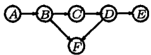
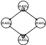
Consider for example the Bayesian network indicated in figure 1. If A is instantiated and no evidence has been entered to DAG4, then DAG�, DAG2, and DAGa are independent, and we need only sent mes sages down to DAG4. An on-line triangulation of this scenario will result in a much simpler set of junction trees than the off-line produced junction tree. To ex ploit the specific independences, we need a very ef ficient algorithm for detecting independences and to perform an efficient triangulation based on these inde pendences. In particular, as the problem of optimal triangulation is N P-complete, there is not much hope that a method requiring on-line triangulation can out perform the "standard" methods for large networks, and improved performance for small networks is not particularly interesting.
We may relax the requirement to the updating al gorithm such that we are only interested in updated probabilities for a very small set of variables. In that case the SPI method [Shachter et al., 1990] and the bucket sort algorithm [Dechter, 1996] can utilize spe cific independences, as they consist of a collect oper ation only, where the variables are successively elimi nated by multiplying the functions involving A (say)
and marginalizing A out of this product. These meth ods, however, are not able to update all variables effi ciently.
In this paper we propose a compromise between off-line triangulation and on-line exploitation of specific inde pendences. We call the method lazy propagation as the bulk of the method is lazy evaluation of the potentials for cliques and separators. That is, we work with an off-line produced junction tree, where we have allowed ourselves to use much time on finding a small junc tion tree. Now, instead of multiplying the conditional probability distributions for the various cliques, we de termine on-line which potentials to multiply when a message is to be produced. Thereby, when a message is to be produced, only the required functions are mul tiplied. An effect of this scheme is that d-separation properties induced by evidence are automatically ex ploited.
The rest of the paper is organized in the following way. Section 2 describes the lazy propagation scheme in de tail. In section 3 we present results from a series of real-time tests performed. A discussion of the results is given in section 4, and in section 5 we illustrate how d-separation properties are automatically exploited.
2 Methods
We briefly review the HUGIN and the Shafer-Shenoy algorithms. For more elaborate presentations, see the references above.
A Bayesian network consists of a graph G = (V, £) and a probability distribution P. G is a directed acyclic graph, Vis the set of variables (which are assumed to be discrete), and £ is the set of edges connecting the variables. The probability distribution P factorizes on G such that:
where pa(V) is the parent set of V. The secondary structures used by the HuGIN and Shafer-Shenoy ar chitectures are constructed from G.
A junction tree representation of a Bayesian network G is constructed by moralization and triangulation of G. The nodes of the junction tree correspond to cliques of the triangulated graph. A clique is a max imal connected subgraph of the triangulated graph. The cliques of the junction tree are connected by sep arators such that the so-called junction tree property holds. The junction tree property insures that when ever two cliques Ci and Cj are connected by a path, the intersection, Ci n Ci is a subset of every clique and separator on the path. To each clique C and each separator S we associate potentials ¢c and ¢s, re spectively. ¢c and ¢s are functions having the vari ables of C and S as domains. Each variable, V, in the Bayesian network has a conditional probability distri bution P(V I pa(V)). Every distribution is assigned to a clique such that the domain of the distribution is a subset of the clique domain. The set of distribu tions assigned to a clique, C, are combined to form the potential function 1/Jc. Initially the potentials of the junction tree are given as:
for each clique, C, and each separator, S.
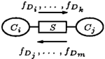
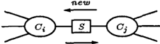
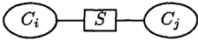
The propagation of evidence in the HUGIN architecture is based on the operation of absorption. Assume Ci and Ci to be neighboring cliques in a junction tree with S as separator, see figure 2. We say that Cj absorbs from ci if we:
- calculate ¢8 = L ¢c;; G;\S
- giveS the potential ¢*s;
- give Ci the potential ¢c. = ¢a. �s . ' ' 'f' S
The absorption operation is used when a message is sent from one clique to another. Messages flow in two recursive phases, and the flow is controlled by choos ing a root clique of the junction tree. The first phase is initiated by collecting evidence to the root and the second phase is initiated by distributing evidence from the root. Collection of evidence to a clique C is done by collecting evidence to all the children of C followed by absorption of evidence from each child. Similarly, distribution of evidence from a clique amounts to ab sorption of evidence into each child followed by distri bution of evidence from the child. After a full round of message passing a message has been sent in each direction along every separator in the junction tree.
The Shafer-Shenoy algorithm can perform inference in a junction tree. The reader should notice that the Shafer-Shenoy algorithm propagates evidence faster in binary join trees than in junction trees [Shenoy, 1997). The Shafer-Shenoy inference architecture differs from
·
the HUG IN architecture in a number of ways. First, the flow of messages is not controlled by choosing a root of the junction tree. A clique sends asynchronously a message to one of its neighbors when messages from all other neighbors have been received. Second, the clique potentials are not updated during propagation of evidence instead each separator holds two messages. One for each direction. Third, no division of poten tials is performed. Consider figure 2 once again. The Shafer-Shenoy message, </JG;-tC;' sent from ci to Cj is calculated as:
where 'lj;0, is the clique potential of ci and Nc, is the set of neighbors to ci.
After a full round of message passing in the Shafer Shenoy architecture each separator holds two mes sages. The clique potential </Jc, can be obtained by taking the product of all messages sent to ci and 'lj; c, 0
The message passing scheme for asynchronous firing corresponds to the scheme of CollectEvidence followed by DistributeEvidence. The root is, however, chosen randomly. Let the separator, S, between cliques Ci and Ci be the first separator over which messages are sent in both directions, see figure 3. Before Cj sent the message, new, over S, it has received a message from all its neighbors. This is equivalent to collecting evidence to C3· Sending messages from Ci to all its neighbors is equivalent to distributing evidence from Ci.
The SPI algorithm and the bucket elimination algo rithm do not perform inference based on a secondary structure. Both algorithms are most advantageously used if the reasoning is focused in the sense that only the posterior probability distributions of a small set of target variables are to be calculated. The basic idea behind the SPI and the bucket elimination algo rithms is to consider only variables relevant to reason ing about the target set. The variables relevant for a query can be determined from the original Bayesian network by an algorithm which runs in time linear in the number of arcs in the graph. The posterior distri bution of the target set is equal to the product of the distributions of the relevant nodes marginalized down to the target set.
2.1 Lazy Propagation
The basic idea behind lazy propagation is to take ad vantage of two important properties of the potentials associated with the nodes of the Bayesian network:
- the d-separation criterion applies to the poten tials.
Instead of combining the probability distributions as sociated with a clique to obtain the clique potential, we keep the clique potential in factored form, and we change the content of messages passed between cliques in the junction tree. Instead of sending a message con sisting of one potential with the set of separator vari ables as domain, we sent a message consisting of a set of potentials all having domains which are subsets of the separator domain. Messages can flow as in the asynchronous firing scheme or may be controlled by choosing a root as in the HUGIN architecture.
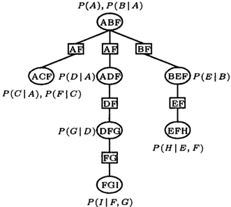
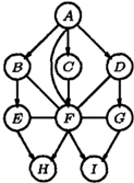
Consider the Bayesian network shown in figure 4 and the corresponding junction tree shown in figure 5. As sume that variable A is i nstantiated by evidence. Each potential with A in its domain has the domain de creased by A. If we assume potentials to be repre sented as tables, then P* is the subtable of P corre sponding to the instantiation of A.
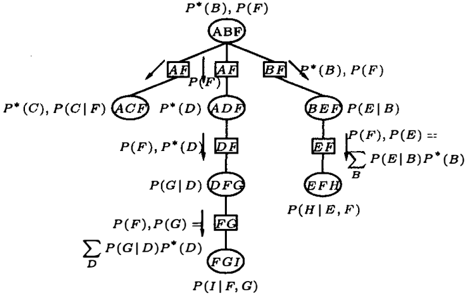
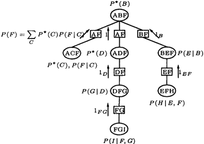
In figure 6 we follow the flow of messages from the leaves of the junction tree towards ABF in the lazy propagation scheme. The message flow corresponds to collecting evidence to ABF in the HUGIN archi tecture. Assume that the first leaf to sent a message is EF H. The potential associated with this clique is P(H IE, F). Variable H has to be eliminated, but no calculations are required as LH P(H I E, F) = lEF·
P(A), P(B I A)
The same argument is used when messages are sent from BEF, FGI, DFG, and ADF. The last clique to send a message is AC F. AC F has P* (C) and P( F I C) associated, and variable C is eliminated by taking the product of the two potentials and then marginalizing down to F.
P*(B)
At the end of the inward pass, potentials P*(B) and P(F) are associated with ABF. In figure 7 we fol low the message flow in the opposite direction. The message sent from ABF to ACF is an empty message as none of the potentials associated with AB F needs to be sent to ACF. P(F) is the only potential rele vant, but it was sent in the opposite direction during the inward pass of the algorithm ( in HUGIN terms it is divided out, in Shafer-Shenoy terms it shall not be transmitted ) . The message sent from ABF to ADF consists of the potential P(F) as no other potentials are relevant for the subtree rooted at ADF. The po- tentials sent from ADF to DFG are P(F) and P*(D). At DFG we have to combine P*(D) and P(G I D) and marginalize D out to obtain the message to send to FGI. BEF is the last child of ABF to receive a message, and the message sent consists of P*(B) and P(F). Finally, a message containing P(F) and P(E) = LBP(EIB)P*(B) is sent to EFH.
P*(B), P(F)
It is not necessary to send the potentials containing only ones. We have included these potentials in the description to make the explanation clear. So, for this example we only performed three marginalizations and all of them involved only two variables.
The HUGIN architecture imposes a division of separa tor potentials as described above. The lazy propaga tion scheme does not require this division, because the combination of potentials is postponed. Consider the two neighboring cliques shown in figure 8, and assume that the message sent from Ci to Cj over the separator S consists of the potentials !D;, ... , fD�o and assume the message sent in the opposite direction to consist of the potentials f D; , ... , f Drn. None of the poten tials !Do ... , fD�o are involved in any marginalization when sending from Cj to ci. That is, !D;, ... , !D. c !D;, ... , f Drn, and the division operation required in HUGIN propagation quite simply amounts to discard ing !Do ... , fD�o from fD;, ... , !Dm. So, lazy propa gation dissolves the difference between HUGIN propa gation and Shafer-Shenoy propagation.
3 Empirical Results
We have tested the lazy propagation scheme to inves tigate how performance varies with the number of in stantiated variables. To get an idea of the performance compared to standard schemes we have implemented Shafer-Shenoy as well as HUGIN propagation. The schemes implemented do only perform propagation. That is, the final step after propagation to marginalize the clique potentials down to each variable is not per formed. Also, we have not implemented various speed up features, like binary join trees or 0-compression.
Number of evidencevariables
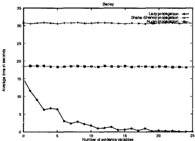
Figure 10: A plot of the average time cost of propa gating evidence in the Barley network as a function of the number of variables instan tiated.
The tests were performed on a Sun Ultra-2 worksta tion with two 300 MHz UltraSPARC-1 CPU's running Solaris 2.6 (SunOS 5.6). Each CPU has a 0.5 MB 12 cache. The total RAM on the system is 1024 MB.
The algorithms were tested on different real-world Bayesian networks with different sizes of evidence sets.
For a given Bayesian network we performed 50 prop agations of evidence with the size of the evidence set fixed, but where the evidence variables were chosen at random before each propagation. The number of evi dence variables varied from 0 to 50. Figure 9 describes four of the Bayesian networks and corresponding junc tion trees used for the tests.
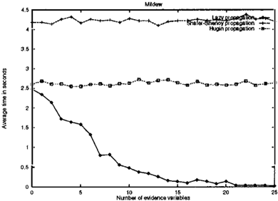
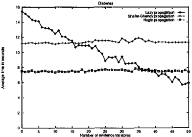
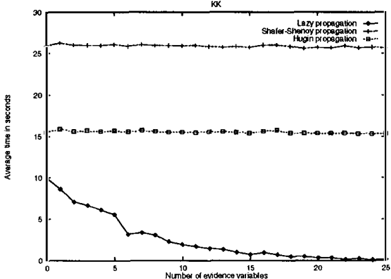
Figures 10, 11, 12, and 13 show the average time cost of propagating evidence with the three schemes as a function of the number of variables instantiated in the Barley, the KK, the Diabetes, and the Mildew net works. The figures show that the average time cost of HUGIN propagation for this implementation is always smaller than the average time cost of Shafer-Shenoy propagation, and that the average time cost of lazy propagation decreases considerably as the number of instantiated variables increase.
The average time cost of lazy propagation in the Bar ley, KK, and Mildew networks is smaller than the time cost of the other propagation algorithms even when no variables are instantiated. On average lazy prop agation in the Diabetes network becomes faster than Shafer-Shenoy propagation when 16 variables are in stantiated, and faster than HUGIN propagation when 39 variables are instantiated.
4 Discussion
The experiments indicate that although some evidence may increase time costs, the overall effect of instanti ating variables is a decrease of time costs, and with many variables instantiated, lazy propagation outper forms standard propagation schemes.
It seems that time costs are in the same order of magnitude with no instantiated variables for all three
| node potential size | clique state space size | clique neighbors | |||||||||
|---|---|---|---|---|---|---|---|---|---|---|---|
| Network | nodes | min | max | f.l- | cliques | min | max | f.l- | min | max | f.l- |
| KK | 50 | 2 | 32256 | 2768.1 | 38 | 40 | 5806080 | 397780.2 | 1 | 4 | 1.9 |
| Barley | 48 | 2 | 40320 | 2712.1 | 36 | 216 | 7257600 | 481637.5 | 1 | 4 | 1.9 |
| Diabetes | 413 | 5 | 7056 | 1116.4 | 337 | 495 | 190080 | 30906.3 | 1 | 3 | 2.0 |
| Mildew | 53 | 3 | 280000 | 15633.1 | 29 | 336 | 1756800 | 144133.0 | 1 | 3 | 1.9 |
schemes, and a rather small set of instantiated vari ables will yield lazy propagation faster than the stan dard schemes. Further research is needed to quantify these statements
We have only performed a limited number of tests to investigate how much the space costs are reduced. These tests indicate that the space costs are reduced considerably. This is expected as clique and separator potentials are represented in factored form. Time and space prevents us from giving a thorough elaboration of this topic.
We have done little to speed-up the calculations of a message in the test implementation of lazy propaga tion. When a message has to be sent from one clique to another some variables have to be marginalized out. If we consider the domain graphs of the potentials rel evant to the calculation of the message, then we are faced with a problem similar to the overall problem. That is, we have to calculate the joint probability of a set of nodes in the domain graph. Here any infer ence algorithm can be used. In the test implementa tion all relevant potentials are arranged in a list and variables not in the separator domain are eliminated one by one. Variables are eliminated according to the following peeling algorithm:
- For each variable, V, not in the separator do main calculate the domain size of the potential obtained, if V is the next variable eliminated. A variable, V, is eliminated by combining all poten tials including V in the domain and marginalizing V out.
- Choose the next variable to eliminate as a vari able resulting in the smallest domain size of the potential obtained.
The algorithm is similar to the minimum clique weight heuristic for triangulation, but it is a little different. We do not always eliminate a variable V right away even though its neighbors form a complete graph as in the minimum clique weight heuristic. V is only elimi nated right away if there is only one relevant potential containing V.
The performance of the lazy propagation scheme de pends very much on the topology of the junction tree. If the state spaces of the cliques and separators are large, the lazy evaluation architecture tends to be faster than the other two architectures for small sets of evidence. Sometimes the lazy evaluation architecture is faster even when no variables are instantiated. On the other hand, when the state spaces of the cliques and separators are small, large sets of evidence vari ables are required before the algorithm becomes faster.
If a Bayesian network has many nodes without par ents or many nodes without children, then speed-up is available even when no variables are instantiated. Let V be a variable without parents, then the marginal probability distribution of V can be sent over sepa rators including V right away. Let W be a variable without children and assume that the potential of W is associated with clique C. When a message is sent from C over a separator not including W and W has not received evidence, then no calculations are neces sary to eliminate Was:
This also applies in the more general case. That is, marginalizing out all head variables of a potential will
result in a unity potential with the tail variables as domain.
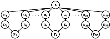
Some sets of evidence decrease the performance of lazy propagation. Consider the Bayesian network shown in figure 14. A junction tree constructed from this network will contain cliques of the form DiEiFi for i = 1, ... , 35, and these cliques are the only cliques containing Fi . No message has to be sent from a DiEiFi clique if variable Fi is not instantiated. If Fi is instantiated, then a message has to be sent from the DiEiFi clique. The lazy evaluation algorithm on average (n = 50) uses 4.2 seconds to propagate evi dence when no variables are instantiated and 5.4 sec onds when variables F1, ... , F35 are instantiated.
The concept of barren nodes was intro duced in ( Shachter, 1986) and are defined in ( Lin and Druzdzel, 1997) as nodes which are neither evidence nor target nodes and have no descen dants or only barren descendants. According to this definition no nodes are barren in the lazy evaluation architecture as we are concerned with calculating the posterior probability distribution of all variables in the Bayesian network. The property of barren nodes exploited by algorithms such as the SPI algorithm is that barren nodes have no impact on the posterior probability distribution of the nodes in the target set. This property is exploited in the lazy propagation scheme as described in the next section.
5 d-separation and Lazy Propagation
Lazy propagation utilizes automatically d-separation properties induced by evidence. To illustrate this, con sider the Bayesian network, N, in figure 15.
N has the properties that initially A and E are not d-separated. If C is instantiated, then A and E are d separated, but if C and F are instantiated, then A and
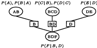
E are not d-separated. In figure 16 a junction tree for N is shown. For the internal elimination order in the cliques we use the peeling algorithm from section 4.
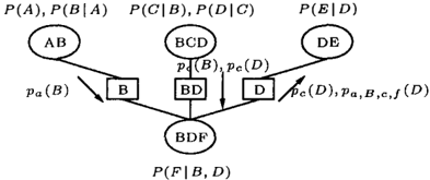
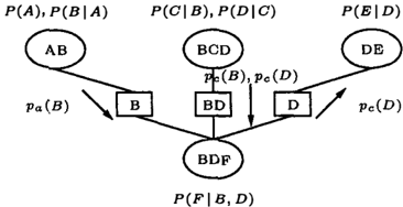
Now, assume that A is instantiated to a. In figure 17 we illustrate the flow of potentials towards the clique DE . The index of the potentials in the figure indi cates the variables rele � ant for the calculation of the potentials. Index a indicates that the evidence A= a is relevant for the potential.
As can be seen from figure 17, the evidence A = a is relevant fot the updating of E . On the other hand, F is irrelevant forE , and this has caused a computational saving as the marginalization ofF is costless. The cost of propagation is close to the cost of propagating in a junction tree for N \{ F } .
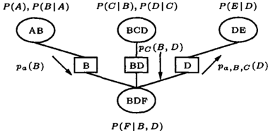
Next, assume that also C is instantiated ( to c ) . The flow of potentials is illustrated in figure 18.
We see that only C =c is relevant forE , and the fact
that E and A are d-separated has yielded substantial savings in the computation. No marginalizations are performed in the propagation.
For completion we illustrate what happens when we furthermore instantiate F to f. Then A and E are not d-separated, and the resource requirements for updat ing DE increase.
6 Conclusion
In this paper we presented an algorithm for proba bilistic inference in Bayesian networks. The algorithm exploits the independences induced by evidence and the direction of the links in the original graph. The performance depends on the topology of the original Bayesian network and the junction tree constructed from it.
The test results show that the algorithm performs in ference faster than both the HUGIN and the Shafer Shenoy algorithms if the size of the set of evidence variables is large enough. It should, however, be em phasized that the performance of the test implemen tations of the Shafer-Shenoy and the HUGIN archi tectures can be improved by exploiting existing tech niques for speeding up the algorithms. Most of these techniques also apply to the lazy evaluation architec ture.
The lazy propagation scheme enlarges the class of tractable Bayesian networks as the space costs of this scheme are smaller than the space costs of the HUG IN and Shafer-Shenoy architectures.
Acknowledgment
Thanks to the anonymous referees for productive re marks and to the DINA-group at Aalborg University (http:/ /www.cs.auc.dk/research/DSS/DINA).
References
[Dechter, 1996] Dechter, R. (1996). Bucket elimina- tion: A unifying framework for probabilistic infer ence. In Horvitz, E. and Jensen, F., editors, Pro ceedings of the Twelfth Conference on Uncertainty in Artificial Intelligence, pages 211-219.
[Jensen, 1995] Jensen, F. V. (1995). Cautious prop agation in Bayesian networks. In Besnard, P. and Hanks, S., editors, Proceedings of the Eleventh Con ference on Uncertainty in Artificial Intelligence, pages 323-328.
[Jensen et al., 1990] Jensen, F. V., Lauritzen, S. L., and Olesen, K. G. (1990). Bayesian updating in causal probabilistic networks by local computations. Computational Statistics Quarterly, 4:269-282.
[Lauritzen and Spiegelhalter, 1988] Lauritzen, S. L. and Spiegelhalter, D. J. (1988). Local computations with probabilities on graphical structures and their application to expert systems. Journal of the Royal Statistical Society, B., 50(2):157-224.
[Lin and Druzdzel, 1997] Lin, Y. and Druzdzel, M. J. (1997). Computational advantages of relevance rea soning in Bayesian belief networks. In Geiger, D. and Shenoy, P., editors, Proceedings of the Thir teenth Conference on Uncertainty in Artificial In telligence, pages 342-350.
[Shachter, 1986] Shachter, R. (1986). Evaluating in fluence diagrams. Operations Research, 34(6) :871-882.
[Shachter et al., 1990] Shachter, R., D'Ambrosio, B., and DelFavero, B. (1990). Symbolic probabilistic inference in belief networks. In Proceedings Eighth National Conference on AI, pages 126-131.
[Shachter, 1990] Shachter, R. D. (1990). An ordered examination of influence diagrams. Networks, 20(5):535-563.
[Shafer and Shenoy, 1990] Shafer, G. R. and Shenoy, P. P. (1990). Probability propagation. Annals of Mathematics and Artificial Intelligence, 2:327-352.
[Shenoy, 1997] Shenoy, P. P. (1997). Binary join trees for computing marginals in the Shenoy-Shafer ar chitecture. International Journal of Approximate Reasoning, 17(2-3) :239-263.