Learning Bayesian Networks: A Unification for Discrete and Gaussian Domains

David Heckerman [email protected]

Dan Geiger [email protected]

August 1995, Revised June 2021

Abstract

We examine Bayesian methods for learning Bayesian networks from a combination of prior knowledge and statistical data. In particular, we unify the approaches we presented at last year's conference for discrete and Gaussian domains. We derive a general Bayesian scoring metric, appropriate for both domains. We then use this metric in combination with well-known statistical facts about the Dirichlet and normal-Wishart distributions to derive our metrics for discrete and Gaussian domains.

Corrections to the original text in red are taken from J. Kuipers, G. Moffa, and D. Heckerman, Addendum on the scoring of Gaussian directed acyclic graphical models. Annals of Statistics 42, 1689-1691, Aug 2014. Other updates to the original are in blue.

1 Introduction

At last year's conference, we presented approaches for learning Bayesian networks from a combination of prior knowledge and statistical data. These approaches were presented in two papers: one addressing domains containing only discrete variables (Heckerman et al., 1994), and the other addressing domains containing continuous variables related by an unknown multivariate-Gaussian distribution (Geiger and Heckerman, 1994). Unfortunately, these presentations were substantially different, making the parallels between the two methods difficult to appreciate. In this paper, we unify the two approaches. In particular, we abstract our previous assumptions of likelihood equivalence, parameter modularity, and parameter independence such that they are appropriate for discrete and Gaussian domains (as well as other domains). Using these assumptions, we derive a domain-independent Bayesian scoring metric. We then use this general metric in combination with well-known statistical facts about the Dirichlet and normal-Wishart distributions to derive our metrics for discrete and Gaussian domains. In addition, we provide simple proofs that these assumptions are consistent for both domains.

Throughout this discussion, we consider a domain U of n variables x 1 , . . . , x n . Each variable may be discrete-having a finite or countable number of states-or continuous. We use lower-case letters to refer to variables and upper-case letters to refer to sets of variables. We write x i = k to denote that variable x i is in state k . When we observe the state for every variable in set X , we call this set of observations a state of X ; and we write X = k X as a shorthand for the observations x i = k i , x i ∈ X . The joint space of U is the set of all states of U . We use p ( X = k X | Y = k Y , ξ ) to denote the generalized probability density that X = k X given Y = k Y for a person with current

state of information ξ [DeGroot, 1970, p. 19]. We use p ( X | Y, ξ ) to denote the generalized probability density function (gpdf) for X , given all possible observations of Y . The joint gpdf over U is the gpdf for U .

We use B s to denote the structure of a Bayesian network, and Π i to denote the parents of x i in a given network. We assume the reader is familiar with Bayesian networks for the case where all variables in U are discrete. Here, we describe a Bayesian-network representation for continuous variables. In particular, consider the special case where all the variables in U are continuous and the joint probability density function for U is a multivariate (nonsingular) normal distribution. In this case, to be in line with more standard notation, we use glyph[vector] x to denote the set of variables U . We have

where glyph[vector] µ is an n -dimensional mean vector, and Σ = ( σ ij ) is an n × n covariance matrix, which must be both symmetric and positive definite. Both glyph[vector] µ and Σ are implicitly functions of ξ . We shall find it convenient to refer to the precision matrix W = Σ -1 , whose elements are denoted by w ij .

This joint density function can be written as a product of conditional density functions each being a normal distribution. Namely,

where µ i is the unconditional mean of x i (i.e., the i th component of glyph[vector] µ ), v i is the conditional variance of x i given values for x 1 , . . . , x i -1 , and b ji is a linear coefficient reflecting the strength of the relationship between x j and x i (e.g., DeGroot, p. 55).

Thus, we may interpret a multivariate-normal distribution as a Bayesian network, where there is no arc from x j to x i whenever b ji = 0, j < i . Conversely, from a Bayesian network with conditional distributions satisfying Equation 3, we may construct a multivariate-normal distribution. We call this special form of a Bayesian network a Gaussian network. The name is adopted from Shachter and Kenley (1989) who first described Gaussian influence diagrams. We note that, in practice, it is typically easier to assess a Gaussian network than it is to assess directly a symmetric positive-definite precision matrix.

The transformations between glyph[vector] v = { v 1 , . . . , v n } and B ≡ { b ji | j < i } of a given Gaussian network G and the precision matrix W of the normal distribution represented by G are well known. In this paper, we need only the transformation from W to { glyph[vector] v, B } . We use the following recursive form given by Shachter and Kenley (1989). Let W ( i ) denote the i × i upper left submatrix of W , glyph[vector] b i denote the column vector ( b 1 i , . . . , b i -1 ,i ), and glyph[vector] b ′ i denote the transpose of glyph[vector] b i . Then, for i > 1, we have

Although Equation 3 is useful for the assessment of a Gaussian network, we shall sometimes find it convenient to write

and W (1) = 1 v 1 .

where m i , i = 1 , . . . , n is defined by

Note that m i is the mean of x i when all of x i 's parents are equal to zero.

As an example, given the three-node network structure x 1 → x 3 ← x 2 , we have b 12 = 0, x 1 = n ( m 1 , 1 /v 1 ) , x 2 = n ( m 2 , 1 /v 2 ) , and x 3 = n ( m 3 + b 13 ( x 1 -m 1 ) + b 23 ( x 2 -m 2 ) , 1 /v 3 ). Also, the precision matrix corresponding to this network structure is given by

Finally, it is important to note that two or more Bayesian-network structures for a given domain can be equivalent in the sense that the structures represent the same set of gpdfs for the domain (Verma and Pearl, 1990). For example, for the three variable domain { x, y, z } , each of the network structures x → y → z , x ← y → z , and x ← y ← z represents the gpdfs where x and z are conditionally independent of y , and are therefore equivalent. As another example, a complete network structure is one that has no missing edges. In a domain with n variables, there are n ! complete network structures. All complete network structures for a given domain represent the same set of gpdfs-namely, all possible gpdfs-and are therefore equivalent. In our proofs to follow, we require the following characterization of equivalent networks, proved by Chickering (in this proceedings).

Theorem 1 (Chickering, 1995) Let B s 1 and B s 2 be two Bayesian-network structures, and R B s 1 ,B s 2 be the set of edges by which B s 1 and B s 2 differ in directionality. Then, B s 1 and B s 2 are equivalent if and only if there exists a sequence of | R B s 1 ,B s 2 | distinct arc reversals applied to B s 1 with the following properties:

1. After each reversal, the resulting network structure contains no directed cycles and is equivalent to B s 2
2. After all reversals, the resulting network structure is identical to B s 2
3. If x → y is the next arc to be reversed in the current network structure, then x and y have the same parents in both network structures, with the exception that x is also a parent of y in B s 1

2 A Bayesian Approach for Learning Bayesian Networks

Our Bayesian approach for learning Bayesian networks can be understood as follows. Suppose we have a domain of variables { x 1 , . . . , x n } = U , and a set of cases { C 1 , . . . , C m } = D where each case is a state of some or of all the variables in U . We sometimes refer to D as a database. We begin with the following random-sample assumption : the database is a random sample from some sample distribution with unknown parameters Θ U , and this sample distribution satisfies the conditionalindependence assertions of some network structure B s for U . We define B h s to be the hypothesis that the sample distribution can be encoded in B s .

Now, suppose that we wish to determine the gpdf p ( C | D,ξ )-the generalized probability density function for a new case C , given the database and our current state of information ξ . Rather than reason about this distribution directly, we assume that the collection of hypotheses B h s corresponding to all network structures for U form a mutually exclusive and collectively exhaustive set 1 and

1 We comment on this assumption in the following section.

compute

In practice, it is impossible to sum over all possible network structures. Consequently, we attempt to identify a small subset H of network-structure hypotheses that account for a large fraction of the posterior probability of the hypotheses. Rewriting the previous equation using the fact that p ( B h s | D,ξ ) = p ( D,B h s | ξ ) /p ( D | ξ ), we obtain

where c is the normalization constant 1 / [ ∑ B h s ∈ H p ( D,B h s | ξ )]. From this relation, we see that only the relative posterior probabilities p ( D,B h s | ξ ) matter. Thus, we compute this relative posterior probability, or alternatively, a Bayes' factor -p ( B h s | D,ξ ) /p ( B h s 0 | D,ξ )-where B s 0 is some reference structure such as the empty graph. We call methods for computing these relative posterior probabilities Bayesian scoring metrics.

Extending the Bayesian analysis, we use Θ Bs to denote the parameters of the sample distribution encoded in the network structure B s given hypothesis B h s . That is, the parameters Θ Bs determine the local gpdfs in B p . From the rules of probability, we have

The assessment of the network-structure priors p ( B h s | ξ ) is treated elsewhere (e.g., Buntine, 1991, and Heckerman et al., 1995). In the following section, we introduce a set of assumptions that simplifies the assessment of the network-parameter priors p (Θ Bs | B h s , ξ ). In the remainder of this section, we show how to compute p ( D | Θ Bs , B h s , ξ ).

A method for computing this term follows from our random-sample assumption. Namely, given hypothesis B h s , it follows that D can be separated into a set of random samples, where these random samples are determined by the structure of B s . First, let us examine this decomposition when all the variables in U are discrete. Let θ X = k X | Y = k Y denote the parameter corresponding to the probability p ( X = k X | Y = k Y , ξ ), where X and Y are disjoint subsets of U . In addition, let x il and Π il denote the variable x i and the parent set Π i in the l th case, respectively; and let D l denote the first l -1 cases in the database. Then, given B h s , we know that the observations of x i in those cases where Π il = k Π i is a random sample with parameters Θ x il | Π il = k Π i . That is,

where k Π i is the state of Π il consistent with { x 1 l = k 1 , . . . , x ( i -1) l = k i -1 } . Using Equation 9, we can compute p ( D | Θ Bs , B h s , ξ ) for any database D and network structure B s for discrete domain U .

Now consider a domain of continuous variables glyph[vector] x = { x 1 , . . . , x n } , and suppose the database D is a random sample from a multivariate-normal distribution with parameters Θ U = { glyph[vector] µ, W } . From our discussion in Section 1, it follows that, given hypothesis B h s , each variable x i is a random sample from a normal distribution with mean m i + ∑ x j ∈ Π i b ji x j and variance v i . Thus, with Θ Bs = { glyph[vector] m,B,glyph[vector] v } , we have

Using Equation 10, we can compute p ( D | Θ Bs , B h s , ξ ) for any D and B s in a Gaussian domain.

The generalization of Equations 9 and 10 is straightforward, and we state it as our first formal assumption.

Assumption 1 (Random Sample) Let D = { C 1 , . . . , C m } be a database, and B s be a network structure for U determined by variable ordering ( x 1 , . . . , x n ) . Let Θ( x i , Π i ) denote the parameters of the network associated with variable x i . Then, for all variables x i ∈ U ,

where f is some function of the parameters Θ( x i , Π i ) and the database entries x il and Π il .

In the discrete case, we have Θ( x i , Π i ) = Θ x i | Π i , and f (Θ( x i , Π i ) , x il , Π il ) = Θ x il | Π il . In the Gaussian case, we have Θ( x i , Π i ) = { m i , v i , glyph[vector] b i } , and f (Θ( x i , Π i ) , x il , Π il ) = n ( m i + ∑ x j ∈ Π i b ji x jl , 1 /v i ).

3 Informative Priors

In this section, we derive a general approach for assessing the network-parameter priors p (Θ Bs | B h s , ξ ). Our derivation is based on four assumptions that are abstracted from our previous work.

Assumption 2 (Likelihood Equivalence) Given two network structures B s 1 and B s 2 such that p ( B h s 1 | ξ ) > 0 and p ( B h s 2 | ξ ) > 0 , if B s 1 and B s 2 are equivalent, then p (Θ U | B h s 1 , ξ ) = p (Θ U | B h s 2 , ξ ) .

Informally, the assumption states that the observation of a database does not help to discriminate equivalent network structures. We note that an equivalent way to state likelihood equivalence is that p ( D | B h s 1 , ξ ) = p ( D | B h s 2 , ξ ) for all databases D , whenever B s 1 and B s 2 are equivalent. 2

The motivation for this assumption is different for acausal Bayesian networks-Bayesian networks that represent only assertions of conditional independence-and causal Bayesian networks. For acausal networks, likelihood equivalence is not an assumption, but rather a consequence of our definition of B h s . In particular, recall that the hypothesis B h s is true iff the parameters Θ U satisfy the conditional independence assertions of B s . Therefore, by definition of network-structure equivalence, if B s 1 and B s 2 are equivalent, then B h s 1 = B h s 2 . 3 For example, in the domain { x 1 , x 2 , x 3 } , the equivalent network structures x 1 → x 2 → x 3 and x 1 ← x 2 ← x 3 both correspond to the assertion θ x 1 ,x 3 | x 2 = θ x 1 | x 2 θ x 3 | x 2 . Consequently, B h x 1 → x 2 → x 3 = B h x 1 ← x 2 ← x 3 . This property, which we call hypothesis equivalence , implies likelihood equivalence. We note that, given hypothesis equivalence, we should score equivalence classes of network structures-not individual network structures-when learning acausal Bayesian networks.

For causal Bayesian networks, we must modify the definition of B h s to include the assertion that each nonroot node in B s is a direct causal effect of its parents. Consequently, the property of hypothesis equivalence is contradicted by the new definition. Nonetheless, we have found that the assumption of likelihood equivalence is reasonable for learning causal networks in many domains. (For a detailed discussion of this point, see Heckerman in this proceedings.)

The next assumption was adopted implicitly in our previous work.

2 We assume this equivalence is well known, although we have not found a proof in the literature.

3 We note that there is a flaw with our definition of B h s for acausal Bayesian networks. In particular, the definition implies that hypotheses associated with different network-structure equivalence classes will not be mutually exclusive. For example, in the two-binary-variable domain, the hypotheses B h xy and B h x → y (corresponding to the empty network structure, and the network structure x → y , respectively) both include the possibility θ xy = θ x θ y . This flaw is potentially troublesome, because mutual exclusivity is important for our Bayesian interpretation of network learning (Equation 2). Nonetheless, because the densities p (Θ Bs | B h s , ξ ) must be integrable and hence bounded, the overlap of hypotheses will be of measure zero, and we may use Equation 2 without modification. For example, in our twobinary-variable domain, given the hypothesis B h x → y , the probability that B h xy is true (i.e., θ y = θ y | x ) has measure zero.

Assumption 3 (Structure Possibility) Given a domain U , p ( B h sc | ξ ) > 0 for all complete network structures B sc .

As we shall see, the assumption allows us to make good use of the property of likelihood equivalence. Although it is an assumption of convenience, we have found it to be reasonable for many real-world network-learning problems.

The remaining two assumptions are abstractions of assumptions made either explicitly or implicitly by all researchers who have considered Bayesian-network learning (e.g., Cooper and Herskovits, 1991, 1992; Buntine, 1991; Spiegelhalter et al., 1993). These assumptions are made mostly for computational convenience, although they are reasonable for many domains.

Assumption 4 (Global Parameter Independence) For all network structures B s ,

Assumption 4 says that the parameters associated with each variable in a network structure are independent. This assumption was first introduced under the name of global independence by Spiegelhalter and Lauritzen (1990).

Assumption 5 (Parameter Modularity) Given two network structures B s 1 and B s 2 such that p ( B h s 1 | ξ ) > 0 and p ( B h s 2 | ξ ) > 0 , if x i has the same parents in B s 1 and B s 2 , then

For example, in our two-binary-variable domain, x has the same parents (none) in the network structure x → y and the structure contains no arc. Consequently, the probability density for Θ( x, ∅ ) would be the same for both of these structures. We call this property parameter modularity, because it says that the densities for parameters Θ( x i , Π i ) depend only on the structure of the network that is local to variable x i -namely, on the parents of x i .

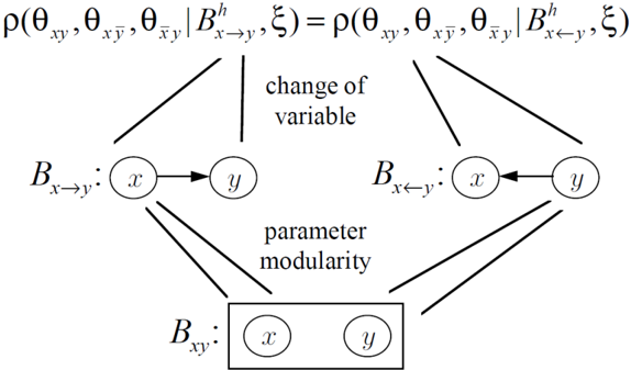
Given Assumptions 2 through 5, we can construct the priors p (Θ Bs | B h s , ξ ) for every network structure B s in U from the single prior p (Θ U | B h sc , ξ ), where B sc is any complete network structure for U . As an illustration of this construction, consider again our two-binary-variable domain. Given the prior density p ( θ xy , θ x ¯ y , θ ¯ xy | B h x → y , ξ ), we construct the priors p (Θ Bs | B h s , ξ ) for each of the three network structures in the domain. First, consider the network structure x → y . The joint-space parameters and parameters for this structure are related as follows:

Thus, we may obtain p ( θ x , θ y | x , θ y | ¯ x | B h x → y , ξ ) from the given density by changing variables:

where J x → y is the Jacobian of the transformation

The Jacobian J B sc for the transformation from Θ U to Θ Bsc in an arbitrary discrete domain is given in Section 5.1.

Next, consider the network structure x ← y . By Assumption 3, the hypothesis B h x ← y is also possible, and, by likelihood equivalence, we have p ( θ xy , θ ¯ xy , θ x ¯ y | B h x ← y , ξ ) = p ( θ xy , θ ¯ xy , θ x ¯ y | B h x → y , ξ ). Therefore, we can compute the density for the network structure x ← y using the Jacobian J x ← y = θ y (1 -θ y ).

Finally, consider the empty network structure. Given the assumption of global parameter independence, we may obtain the densities p ( θ x | B h xy , ξ ) and p ( θ y | B h xy , ξ ) separately. To obtain the density for θ x , we first extract p ( θ x | B h x → y , ξ ) from the density for the network structure x → y . This extraction is straightforward, because, by global parameter independence, the parameters for x → y must be independent. Then, we use parameter modularity, which says that p ( θ x | B h xy , ξ ) = p ( θ x | B h x → y , ξ ). To obtain the density for θ y , we extract p ( θ y | B h x ← y , ξ ) from the density for the network structure x ← y , and again apply parameter modularity. The approach is summarized in Figure 1.

In general, we have the following construction.

Theorem 2 Given domain U and a probability density p (Θ U | B h sc , ξ ) where B sc is some complete network structure for U , Assumptions 2 through 5 determine p (Θ Bs | B h s , ξ ) for any network structure B s in U .

We note that our construction assumes that Assumptions 2 through 5 are consistent. We demonstrate consistency in Section 7.

4 A General Metric for Complete Data

In this section, we derive a general metric from Assumptions 1 through 5 and the following additional assumption:

Assumption 6 (Complete Data) The database is complete. That is, it contains no missing data.

We make this assumption only as a computational convenience. The reader should recognize that random-sample assumption and the informative priors developed in Section 3 can be used in conjunction with well-known statistical techniques to score incomplete databases as well. Such

techniques include filling in missing data based on the data that is present [Titterington, 1976, Spiegelhalter and Lauritzen, 1990], the EM algorithm [Dempster et al., 1977], and Gibbs sampling [Madigan and Raftery, 1994].

Given our assumptions, we obtain the following lemmas. 4

Lemma 3 (Posterior Parameter Independence) Given the random-sample assumption (Assumption 1), global parameter independence (Assumption 4), and the assumption of no missing data (Assumption 6), we have

for all network structures B s ( p ( B h s | ξ ) > 0 ) and databases D .

Lemma 4 (Posterior Parameter Modularity) Given the random-sample assumption (Assumption 1), global parameter independence (Assumption 4), parameter modularity (Assumption 5), and the assumption of no missing data (Assumption 6), if x i has the same parents in any two network structures B s 1 and B s 2 ( p ( B h s 1 | ξ ) > 0 , p ( B h s 2 | ξ ) > 0 ), then

for all databases D .

In the following lemma and in subsequent discussions, we need the notion of a database D restricted to X ⊆ U -that is the projection of database D onto the subset X -denoted D X . For example, given domain U = { x 1 , x 2 , x 3 } and database D = { C 1 = { x 1 = 1 , x 2 = 2 , x 3 = 1 } , C 2 = { x 1 = 2 , x 2 = 2 , x 3 = 1 }} , we have D { x 1 ,x 2 } = { C 1 = { x 1 = 1 , x 2 = 2 } , C 2 = { x 1 = 2 , x 2 = 2 }} .

Lemma 5 Let X be a subset of U , and B sc ( p ( B h sc | ξ ) > 0 ) be a complete network structure for any ordering where the variables in X come first. Given the random-sample assumption (Assumption 1), global parameter independence (Assumption 4), and the assumption of no missing data (Assumption 6),

for all databases D .

Readers familiar with the concept of d-separation will recognize that Lemmas 3 and 5 can be readily obtained from graphical manipulations applied to the Bayesian-network representation of the random-sample assumption and the assumption of global parameter independence.

We can now derive the general metric.

Theorem 6 Given a domain U , let B s be any network structure for U and B sc be a some complete network structure for U . Then, given Assumptions 2 through 6,

for any database D .

4 The proofs are simple and are omitted.

Proof: From the rules of probability, we obtain

For every x i with parents Π i in B s , let B SC, Π i ,x i be a complete network structure with variable ordering Π i , x i followed by the remaining variables. By Assumption 3, p ( B SC, Π i ,x i | ξ ) > 0. Using Assumption 1 and Lemmas 3 and 4, we get

Decomposing the integral over Θ Bs into integrals over the individual parameter sets Θ( x i , Π i ), and performing the integrations, we have

Also, using Lemma 5, we obtain

By likelihood equivalence, we have that p ( D | B SC, Π i ,x i , ξ ) = p ( D | B h sc , ξ ). Consequently, for any subset X of U , we obtain p ( D X | B SC, Π i ,x i , ξ ) = p ( D X | B h sc , ξ ) by summing over the variables in D U \ X . Applying this result to Equation 15, we get Equation 14. glyph[square]

We call Equation 14 the Be ( B ayesian likelihood e quivlent) metric.

5 Special-Case Metrics

Our general metric is powerful, because it tells us that if we know how to compute p ( D X | B h sc , ξ ) for any subset X of U under the assumption that the domain contains no structure (i.e., there are no independencies), then we can compute the probability of any database when there is structure. Therefore, the Be metric allows us to leverage much of the work in the statistics literature, as statisticians have long dealt with the former problem. In this section, we illustrate this claim by deriving likelihood-equivalent metrics for the discrete and Gaussian cases.

5.1 The BDe Metric

Suppose all variables in U are discrete. Recall that we use θ X = k X | Y = k Y denote the multinomial parameter corresponding to probability p ( X = k X | Y = k Y , ξ ). In addition, we use Θ X | Y denote the

collection of parameters θ X = k X | Y = k Y for all states of sets X and Y . If Y is empty, we simply write Θ X . Thus, for example, Θ U = Θ x 1 ,...,x n represents the multinomial parameters of the joint space of U .

Let us assume that the parameter set Θ U has a Dirichlet distribution when conditioned on a hypothesis corresponding to some complete network structure B sc :

where N ′ B sc is the effective sample size of the Dirichlet distribution associated with a complete network structure B sc . DeGroot (1970, p. 50) shows that, for any subset X of U , Θ X also has a Dirichlet distribution:

Now, it is a well-known statistical result that, if a discrete variable x with r states has a Dirichlet distribution with exponents N ′ 1 -1 , . . . , N ′ r -1, then

where D is a database for variable x and N k is the number of times x takes on state k in D . Also, because U is discrete, any subset X of U can also be thought of as a single discrete variable with ∏ x i ∈ X r i states. Therefore, Equations 17 and 18 allow us to compute each term in the Be metric (Equation 14). To express the resulting metric for a given network structure B s , we use q i = ∏ x i ∈ Π i r i to denote the number of states of Π i in B s , and Π i = j to denote that Π i has assumed the j th state, j = 1 , . . . , q i .

Theorem 7 (BDe Metric) Given domain U , and network structure B s and database D for U , let N ijk denote the number of times that x i = k and Π i = j in the database D ; and let N ij = ∑ r i k =1 denote the number of times that Π i = j in a database D . Then, if p (Θ U | B h sc , ξ ) is Dirichlet with effective sample size N ′ for some complete network structure B sc , and if Assumptions 2 through 6 hold, then

Equations 19 and 20 are the BDe ( B ayesian D irichlet likelihood e quivalent) metric, originally derived in Heckerman et al. (1994).

The assumption that p (Θ U | B h sc , ξ ) is Dirichlet is not as arbitrary as it may seem at first glance. In discrete domains, we can assume not only that the parameters corresponding to each variable are independent, but that the parameters corresponding to each state of every variable's parents are independent. Spiegelhalter and Lauritzen (1990) call this added assumption local independence . Geiger and Heckerman (in this proceedings) show that likelihood equivalence, structure possibility, global and local parameter independence, and the assumption that p (Θ U | B h sc , ξ ) is positive imply that p (Θ U | B h sc , ξ ) must be Dirichlet.

where

5.2 The BGe Metric

Suppose that all variables in U = glyph[vector] x are continuous, and that the database is a random sample from a multivariate-normal distribution. Let us assume that the parameter set { glyph[vector] µ, W } has a normalWishart distribution when conditioned on B h sc for some complete network structure B sc . Namely, assume that p ( glyph[vector] µ | W,B h sc , ξ ) is a multivariate-normal distribution with mean glyph[vector] µ 0 and precision matrix N ′ µ W ( N ′ glyph[vector] µ > 0); and that p ( W | B h sc , ξ ) is a Wishart distribution with N ′ T degrees of freedom ( N ′ T > n -1) and positive-definite matrix T 0 . That is,

where c is a normalization constant [DeGroot, 1970, p. 57].

It is well known that the normal-Wishart distribution is a conjugate family for multivariatenormal sampling (e.g., DeGroot, 1970, p. 178). Given a database D = { glyph[vector] x 1 , . . . , glyph[vector] x m } , let glyph[vector] x m and S m denote its sample mean and scatter matrix, respectively. Then, given the normal-Wishart prior we have described, the posterior density p ( glyph[vector] µ, W | D,B h sc , ξ ) is also a normal-Wishart distribution. In particular, p ( glyph[vector] µ | W,D,B h sc , ξ ) is multivariate normal with mean vector glyph[vector] µ m given by

and precision matrix ( N ′ glyph[vector] µ + m ) W ; and p ( W | D,B h sc , ξ ) is a Wishart distribution with N ′ T + m degrees of freedom and matrix T m given by

From these equations, we see that N ′ glyph[vector] µ and N ′ T can be thought of as effective sample sizes for the normal and Wishart components of the prior, respectively.

Given domain U = { x 1 , . . . , x n } , subset X of U with l elements, and vector glyph[vector] y = ( y 1 , . . . , y n ), let glyph[vector] y X denote the vector formed by the components y i of glyph[vector] y such that x i ∈ X . Similarly, given matrix M , let M X denote the submatrix of M containing elements m ij such that x i , x j ∈ X . It is well known that if D is a random sample from an n -dimensional multivariate-normal distribution whose parameters { glyph[vector] µ, W } have a normal-Wishart distribution with constants glyph[vector] µ 0 , N ′ glyph[vector] µ , T 0 , and N ′ T , then D X is a random sample from an | X | -dimensional multivariate distribution with parameters { glyph[vector] µ X , W X } , and these parameters have normal-Wishart distribution with constants glyph[vector] µ X 0 , N ′ glyph[vector] µ , T X 0 , and N ′ T -n + l . Furthermore, the formula for p ( D | B h sc , ξ ) given the normal-Wishart prior is known (Geiger and Heckerman, 1994). Consequently, the evaluation of p ( D X | B h sc , ξ ) in Equation 14 is straightforward.

Theorem 8 (BGe Metric) Given domain glyph[vector] x = { x 1 , . . . , x n } , assume p ( glyph[vector] µ, W | B h sc , ξ ) is an n -dimensional normal-Wishart distribution with constants glyph[vector] µ 0 , N ′ glyph[vector] µ , T 0 , and N ′ T . Given a database D = { C 1 , . . . , C m } and a subset X of glyph[vector] x with l elements, Assumptions 2 through 6 imply the Be metric, where each term is given by

where

and T m is the matrix of the posterior normal-Wishart distribution given by Equation 23.

The Be metric in combination with Equation 24 defines the BGe ( B ayesian G aussian likelihood e quivalent) metric, originally derived in Geiger and Heckerman (1994). We note that assumptions similar to those used to show the inevitability of the Dirichlet distribution for discrete domains imply that the normal-Wishart assumption is inevitable for Gaussian domains (see Geiger and Heckerman in this proceedings).

The BDe and BGe metrics may be combined to score domains containing both discrete variables and continuous variables. Namely, let U = U d ∪ U c where all variables in U d and U c are discrete and continuous, respectively. Suppose that the observations of U d in the database are a random sample from a multivariate-discrete distribution, and the observations of the U c given each state of U d are a random sample from a multivariate-normal distribution. Finally, suppose that Θ U d has a Dirichlet distribution, and that Θ U c | U d = k has a normal-Wishart distribution for every state k of U d . Then, we can apply the Be metric to any network structure B s where the variables in U d precede the variables in U c , using Equation 18 to evaluate terms for discrete variables, and Equations 24 and 25 to evaluate terms for continuous variables.

6 Informative Priors from a Prior Network

Given our assumptions, p (Θ U | B h sc , ξ ) determines a Bayesian scoring metric. In this section, we discuss the assessment of this distribution.

For discrete domains, we can assess p (Θ U | B h sc , ξ ) by assessing (1) the joint probability distribution for the first cases to be seen in the database p ( U | B h s , ξ ) and (2) the effective sample size N ′ for the domain. Methods for assessing N ′ are discussed in (e.g.) Heckerman et al. (1995). To assess p ( U | B h s , ξ ), we can construct a Bayesian network for the first case to be seen. We call this Bayesian network a prior network. The unusual aspect of this assessment is the conditioning hypothesis B h sc (see Heckerman et al. [1995] for a discussion).

We can assess p (Θ U | B h sc , ξ ) in the Gaussian case using a prior network as well. In this case, however, we require two effective samples sizes ( N ′ glyph[vector] µ > 0 and N ′ T > n -1). The details are discussed in last year's proceedings [Geiger and Heckerman, 1994]. Examples of the assessment of p (Θ U | B h sc , ξ ) for discrete and Gaussian domains, and examples of the metrics that result from these assessments are also given in last year's proceedings.

7 Consistency of the Assumptions

The assumptions of likelihood equivalence, structure possibility, global parameter independence, and parameter modularity may not be consistent. In particular, the assumptions of global parameter independence and modularity are constraints on parameter densities among individual network structures, whereas likelihood equivalence is a constraint on parameter densities among networkstructure equivalence classes. Furthermore, our choices p (Θ U | B h sc , ξ ) is Dirichlet and p ( glyph[vector] µ, W | B h sc , ξ ) is normal-Wishart may not be consistent with the assumptions of likelihood equivalence and global parameter independence. In this section, we demonstrate consistency in each case.

7.1 Consistency of the Dirichlet Assumption

First, we show that the assumption p (Θ U | B h sc , ξ ) is Dirichlet is consistent with the assumptions of likelihood equivalence and global parameter independence for complete network structures.

To see the potential for inconsistency, consider again our approach for constructing priors in the two-binary-variable domain. Suppose we choose the density

where c is a normalization constant. By Equations 12 and 13 we obtain

for the network structure x → y . This density satisfies the assumption of global (and local) parameter independence. Using likelihood equivalence, however, we have for the network structure y → x

This density satisfies neither global (nor local) parameter independence.

When p (Θ U | B h sc , ξ ) is Dirichlet, however, likelihood equivalence implies global (and local) parameter independence for all complete network structures. This result is proved for the two-variable case in Dawid and Lauritzen (1993, Lemma 7.2) and for the general case in Heckerman et al. (1995, Theorem 3), which we summarize here.

Theorem 9 Let B sc be any complete network structure for domain U = { x 1 , . . . , x n } . The Jacobian for the transformation from Θ U to Θ Bsc is

Theorem 10 Given a domain U = { x 1 , . . . , x n } , if the parameters Θ U have a Dirichlet distribution with parameters N ′ x 1 ,...,x n -that is,

then, for any complete network structure B sc in U , the density p (Θ Bsc | ξ ) satisfies global and local parameter independence. In particular,

Proof: The result follows by multiplying the right-hand-side of Equation 27 by the Jacobian in Theorem 9, using the relation θ x 1 ,...,x n = ∏ n i =1 θ x i | x 1 ,...,x i -1 , and collecting powers of θ x i | x 1 ,...,x i -1 . glyph[square]

It is interesting to note that each set of conditional parameters Θ x i | x 1 ,...,x i -1 also has a Dirichlet distribution.

where

7.2 Consistency of the Normal-Wishart Assumption

Next, we show that the assumption p ( glyph[vector] µ, W | B h sc , ξ ) is normal-Wishart is consistent with the assumptions of likelihood equivalence and global parameter independence for complete network structures.

Theorem 11 The Jacobian for the change of variables from W to { glyph[vector] v, B } is given by

Proof: Let J ( i ) denote the Jacobian for the first i variables in W . Then J ( i ) has the following form:

where I k,k is the identity matrix of size k × k . Thus, we have

which gives Equation 30. glyph[square]

Theorem 12 The Jacobian for the change of variables from glyph[vector] µ to glyph[vector] m is given by J glyph[vector] m = 1 .

Proof: From Equation 6, J glyph[vector] m is the determinant of a triangular matrix whose diagonal elements are 1. glyph[square]

Theorem 13 If { glyph[vector] µ, W } has a normal-Wishart distribution given background information ξ , then

Proof: To prove the theorem, we factor p ( glyph[vector] m | glyph[vector] v, B, ξ ) and p ( glyph[vector] v, B | ξ ) separately. By assumption, we know that p ( glyph[vector] µ | W ) is a multivariate-normal distribution with mean µ 0 and precision matrix N ′ glyph[vector] µ W . Transforming this result to conditional distributions for µ i , we obtain

for i = 1 , . . . , n . Letting m 0 i = µ 0 i -∑ i -1 j =1 b ji µ 0 j for each i , we get

Thus, collecting terms for each i and using the Jacobian J glyph[vector] m = 1, we have

In addition, by assumption, we have

so that the determinant in Equation 34 factors as a function of i . Also, Equation 4 implies (by induction) that each element w ij in W is a sum of terms each being a function of glyph[vector] b i and v i . Consequently, the exponent in Equation 34 factors as a function of i . Thus, given the Jacobian J glyph[vector] v,B , which also factors as a function of i , we obtain

Equations 33 and 35 imply the theorem. glyph[square]

7.3 Consistency of Likelihood Equivalence, Structure Possibility, Parameter Independence, and Parameter Modularity

As mentioned, the assumptions of likelihood equivalence, structure possibility, global parameter independence, and parameter modularity may not be consistent. To understand the potential for inconsistency, note that we obtained the Be metric (Equation 14) for all network structures using likelihood equivalence applied only to complete network structures in combination with the assumptions of structure possibility, global parameter independence, parameter modularity. Thus, it could be that the Be metric for incomplete network structures is not likelihood equivalent. Nonetheless, the following theorem shows that the Be metric is likelihood equivalent for all network structures-that is, given structure possibility, global parameter independence, and parameter modularity, likelihood equivalence for incomplete structures is implied by likelihood equivalence for complete network structures. Consequently, the assumptions are consistent.

Theorem 14 (Likelihood Equivalence) If B s 1 and B s 2 are equivalent network structures for domain U , then, for all databases D , p ( D | B h s 1 , ξ ) = p ( D | B h s 2 , ξ ) , where each likelihood is computed by the Be metric (Equation 14).

Proof: By Theorem 1, we know that a network structure can be transformed into an equivalent structure by a series of arc reversals. Thus, we can demonstrate likelihood equivalence in general if we can do so for the case where two equivalent structures differ by a single arc reversal. So, let B s 1 and B s 2 be two equivalent network structures that differ only in the direction of the arc between x i and x j (say x i → x j in B s 1 ). Let R be the set of parents of x i in B s 1 . By Theorem 1, we know that R ∪{ x i } is the set of parents of x j in B s 1 , R is the set of parents of x j in B s 2 , and R ∪{ x j } is the set of parents of x i in B s 2 . Because the two structures differ only in the reversal of a single arc, the only terms in the product of Equation 14 that can differ are those involving x i and x j . For B s 1 , these terms are

whereas for B s 2 , they are

These terms are equal, and consequently, so are the likelihoods. glyph[square]

From Equation 4, we have

Acknowledgments

We thank Peter Spirtes for identifying an error with Equation 24.

References

• [Buntine, 1991] Buntine, W. (1991). Theory refinement on Bayesian networks. In Proceedings of Seventh Conference on Uncertainty in Artificial Intelligence, Los Angeles, CA, pages 52-60. Morgan Kaufmann.
• [Chickering, 1995] Chickering, D. (1995). A transformational characterization of equivalent Bayesian network structures. In this proceedings.
• [Cooper and Herskovits, 1992] Cooper, G. and Herskovits, E. (1992). A Bayesian method for the induction of probabilistic networks from data. Machine Learning , 9:309-347.
• [Cooper and Herskovits, 1991] Cooper, G. and Herskovits, E. (January, 1991). A Bayesian method for the induction of probabilistic networks from data. Technical Report SMI-91-1, Section on Medical Informatics, Stanford University.
• [Dawid and Lauritzen, 1993] Dawid, A. and Lauritzen, S. (1993). Hyper Markov laws in the statistical analysis of decomposable graphical models. Annals of Statistics , 21:1272-1317.
• [DeGroot, 1970] DeGroot, M. (1970). Optimal Statistical Decisions . McGraw-Hill, New York.
• [Dempster et al., 1977] Dempster, A., Laird, N., and Rubin, D. (1977). Maximum likelihood from incomplete data via the EM algorithm. Journal of the Royal Statistical Society , B 39:1-38.
• [Geiger and Heckerman, 1994] Geiger, D. and Heckerman, D. (1994). Learning Gaussian networks. In Proceedings of Tenth Conference on Uncertainty in Artificial Intelligence, Seattle, WA, pages 235-243. Morgan Kaufmann, arXiv:1302.6808.
• [Geiger and Heckerman, 1995] Geiger, D. and Heckerman, D. (1995). A characterization of the Dirichlet distribution with application to learning Bayesian networks. In this proceedings.
• [Heckerman, 1995] Heckerman, D. (1995). A Bayesian approach for learning causal networks. In this proceedings.
• [Heckerman et al., 1994] Heckerman, D., Geiger, D., and Chickering, D. (1994). Learning Bayesian networks: The combination of knowledge and statistical data. In Proceedings of Tenth Conference on Uncertainty in Artificial Intelligence, Seattle, WA, pages 293-301. Morgan Kaufmann.
• [Heckerman et al., 1995] Heckerman, D., Geiger, D., and Chickering, D. (1995). Learning Bayesian networks: The combination of knowledge and statistical data. Machine Learning , to appear.
• [Madigan and Raftery, 1994] Madigan, D. and Raftery, A. (1994). Model selection and accounting for model uncertainty in graphical models using Occam's window. Journal of the American Statistical Association , 89:1535-1546.
• [Shachter and Kenley, 1989] Shachter, R. and Kenley, C. (1989). Gaussian influence diagrams. Management Science , 35:527-550.
• [Spiegelhalter et al., 1993] Spiegelhalter, D., Dawid, A., Lauritzen, S., and Cowell, R. (1993). Bayesian analysis in expert systems. Statistical Science , 8:219-282.

• [Spiegelhalter and Lauritzen, 1990] Spiegelhalter, D. and Lauritzen, S. (1990). Sequential updating of conditional probabilities on directed graphical structures. Networks , 20:579-605.
• [Titterington, 1976] Titterington, D. (1976). Updating a diagnostic system using unconfirmed cases. Applied Statistics , 25:238-247.
• [Verma and Pearl, 1990] Verma, T. and Pearl, J. (1990). Equivalence and synthesis of causal models. In Proceedings of Sixth Conference on Uncertainty in Artificial Intelligence, Boston, MA, pages 220-227. Morgan Kaufmann.