Learning Hidden Markov Models with Geometrical Constraints

Hagit Shatkay•

National Center for Biotechnology Information, NLM/NIH Bethesda, MD

[email protected]

Abstract

Hidden Markov models (HMMs) and partially observable Markov decision processes (POMDPs) form a useful tool for modeling dynamical systems. They are particularly useful for representing environments such as road net­ works and office buildings, which are typical for robot navigation and planning. The work presented here is concerned with acquiring such models. We demonstrate how domain-specific information and constraints can be incorporated into the statistical estimation process, greatly improving the learned models in terms of the model quality, the number of iterations required for con­ vergence and robustness to reduction in the amount of available data. We present new initialization heuristics which can be used even when the data suffers from cu­ mulative rotational error, new update rules for the model parameters, as an instance of generalized EM, and a strat­ egy for enforcing complete geometrical consistency in the model. Experimental results demonstrate the ef­ fectiveness of our approach for both simulated and real robot data, in traditionally hard-to-learn environments.

1 Introduction

Hidden Markov models (HMMs), as well as their general­ ization to partially observable Markov decision processes (POMDPs), model a variety of nondeterministic dynamical systems as probabilistic state-transition systems with dis­ crete states, observations, and possibly actions. In this pa­ per we concentrate on the special case of models in which states can be associated with points in a metric configura­ tion space. These are appropriate in contexts such as of­ fice building, road network, or sewerage system modeling. Specifically, such POMDP models form a useful basis for robot navigation in buildings, providing a sound method for localization and planning [SK95, NPB95, CKK96]. Much of the previous work on planning assumed that the model is acquired manually; such manual acquisition can be very te­ dious and it is often difficult to obtain correct probabilities.

Learning such models automatically is an ultimate goal, both for robustness and in order to cope with new and

*This work was supported by the Brown University Graduate Re­ search Fellowship.

changing environments. Since PO MOP models are a simple extension of HMMs, they can, theoretically, be learned with a simple extension to the Baum-Welch algorithm [Rab89] for learning HMMs. However, without a strong prior con­ straint on the structure of the model, the Baum-Welch al­ gorithm does not perform very well: it is slow to converge, requires a great deal of data, and often becomes stuck in local maxima.

Our work focuses on showing how weak information about the metric relationship between states can be used to sig­ nificantly improve model learning. Such information is usually readily available but is often ignored during the process of learning topological maps. We have previ­ ously shown [SK97, SK98] that the odometric ability of the robot, which allows it to roughly measure its geometric position changes while moving in the environment, can be very useful when learning topological models.

This paper addresses several issues not previously dealt with: It introduces a "lag-behind" estimation procedure that enforces geometrical constraints, while being an in­ stance of generalized EM, new heuristics for choosing an initial model from which the iterative optimization starts, and an update strategy that allows the enforcement of the complete geometrical constraints (additivity), while our earlier work enforced only part of the constraints (anti­ symmetry of the odometry between points). We conclude by empirically demonstrating the effectiveness of our algo­ rithms for learning models of environments that are tradi­ tionally considered hard to learn.

2 Related Work

The work presented here is concerned with learning sta­ tistical models in the context of robot navigation. In the robotics domain it is common to distinguish between two main types of maps: geometric and topological. The former represent the environment in terms of the objects placed in it and their positions. For example, grid-based maps [ME85, Asa91, TBF98] are an instance of the geo­ metric approach. Such maps are the best choice when it is necessary for a robot to know its location accurately in terms of metric coordinates. However, in our environments of interest such as office buildings with corridors and rooms or networks of roads, topological maps [KB91], specifying

：

二

一

the important locations and their connections, suffice. Such maps are typically less complex and support much more ef­ ficient planning than metric maps.

We draw an additional distinction, between world-centric1 maps that provide an "objective" description of the environ­ ment independent of the agent using the map, and robot­ centric models which capture the interaction of a partic­ ular "subjective" agent with the environment. An agent learning a map (such as the grid maps mentioned above), takes into account its own noisy sensors and actuators and tries to obtain an objectively correct map that other agents could use as well; other agents need to compensate for their own limitations when assessing their position according to the map. We take the approach of learning a model that captures the interaction of the agent with the environment. Hence, the noisy sensors and actuators specific to the agent are reflected in the model; this approach allows robust plan­ ning, taking into account the error in sensing and action, (although a different model is likely to be needed for differ­ ent agents). Moreover, topological models support a more general notion of state, possibly including information such as the robot's battery voltage or arm position.

The work most closely related to ours is by Koenig and Simmons [KS96a, KS96b], who learn POMDP models (stochastic topological models) of a robot hallway en­ vironment. To overcome the hardship of learning such a model without initial information they use a human­ provided topological map to start from, and further con­ straints on the structure of the model. A modified ver­ sion of the Baum-Welch algorithm learns the parameters of the model. They also developed an incremental ver­ sion of Baum-Welch that allows it to be used on-line in certain kinds of environments. Their models contain very weak metric information, representing hallways as chains of !-meter segments and allowing the learning algorithm to select the most probable chain length. This method is effective, but results in large models (size is proportional to hallways' length). In contrast, we directly incorporate odometric information into the Baum-Welch algorithm to learn a probabilistic model with both discrete and continu­ ous probabilities.

Probabilistic models are widely used within the AI com­ munity. Such models may allow continuous probabilities, as demonstrated in work on Bayesian networks [HG95], HMMs [GJ97] and stochastic maps [SSC91]. However, that work significantly differs from ours in several ways. Com­ monly, the continuous distributions used are linearthat is - distributions assigning density to each point on the real line so that the area under the density curve, integrated over the whole real line, is 1, (most often the distribution is Gaussian). As pointed out in our earlier work [SK98], di­ rectional data is inherently cyclic, requiring the use of cir­ cular distributions, where for some period 1/J (a real num-

' Thanks to Sebastian Thrun for the terminology.

ber), the density of any point x is the same as that of x+k'I/J, for any integer k. In addition, usually the learned statistical parameters are unconstrained (aside for the obvious con­ straint of being a distribution.) Our approach, which en­ forces geometrical constraints when estimating the param­ eters, requires special precautions to ensure convergence of the iterative reestimation procedure, as demonstrated in the following sections.

3 Models and Assumptions

We describe here the model (and later the algorithms) for learning an HMM, rather than a POMDP. The extension to POMDPs-which we developed and implemented-is tech­ nically straightforward but notationally more cumbersome.

The world is composed of a finite set of states, whose num­ ber is assumed here to be known. The dynamics of the world are described by state-transition distributions, speci­ fying the probability of transitioning from one state to the next. A finite set of possible observations is associated with each state; the observation frequency is described by a probability distribution and depends only on the current state. In our model, observations are multi-dimensional, hence, an observation is a vector of values, each chosen from a finite domain. We assume that observation values are conditionally independent, given the state.

In addition, each state is assumed to be associated with a (not necessarily unique) point in some metric space. When­ ever a state transition is made, encoders on the robot's wheels allow it to record its current pose (position and ori­ entation) relative to its pose in the previous state. It is as­ sumed that the position change (�x. �y) is corrupted with independent 0-mean normal noise, while the orientation change, (�0), is corrupted with independent von Mises­ distributed noise. The von Mises distribution is a circular version of the normal distribution, and its density function is: f (0) = �eKcos(S-�) where�> is a concentraJJ,K. 2-rr /0\ltJ ' tion parameter and Io ( �>) is the modified Bessel function of the first kind and order 0. It is extensively discussed in former work [GGD53, Mar72, SK98].

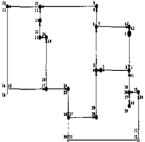
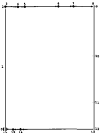
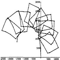
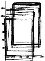
In early work [SK97] we assumed perpendicularity of the corridors that was taken advantage of while the robot col­ lected the data; Odometric readings were recorded with re­ spect to a global coordinate system, and the robot could re-align itself with the origin after each turn. A trajec­ tory of odometry recorded under this assumption by our robot Ramona, along the x and y axes is given in Fig­ ure 1. In contrast, Figure 2 shows a trajectory of the odome­ try recorded without the perpendicularity assumption. The data collected under the latter setting is subjected to cu­ mulative rotational error. In recent work [SK98] we have shown how such data can be handled through state-relative coordinate systems, as explained later in this section. This solution is reflected both in the constraints imposed on the model and in the learning algorithm.

To state the setting formally, a model is a tuple

.>. = (S, 0, A, B, 1r, R), where

• S = {so, . . . , BN-d is a finite set of N states;
• 0 = rt = l 0; is a finite set of observation vectors of length I; the ith element of an observation vector is cho­ sen from the finite set 0;;
• A is a stochastic transition matrix, with A;,j =Pr(q,+1= Bj l q, = s;); os; i , j s; N -1; q, is the state at timet;
• B is an array of l stochastic observation matrices, with Bi,j,o=Pr(V,[i] = oiq,=sj); 1:5 is; I, O:Sj :5 N-1, o E Oj; v; is the observation vector at timet;
• 1r is a stochastic initial probability vector describing the distribution of the initial state; for simplicity it is as­ sumed here to be (0, ... 0, 1, 0, ... , 0), implying that the robot always starts in a designated initial state s;;
• R is a relation matrix, specifying for each pair of states, s; and s i, the mean and variance of the metric relation between them along the x and the y dimensions; e.g. !l[j � Jl(R; , j[x]) is the mean of the x component of the relation between s; and Sj, and (""fi) 2 � 0"2(R;,j[x]), the variance. As shown in earlier work [SK98] R also contains the mean and concentration of the change in heading between the two states, llfj and Kfj· Further­ more, R is geometrically consistent; In a global co­ ordinate system this means that for each component wE {x, y,O}, the relation Jl �b � Jl(Ra , b[w]) must be a directed metric, satisfying the following constraints (referred to as global constraints from here on) for all states a, b, and c:
• <> !l � a = 0;
• <> il�b = -ll't:a (anti-symmetry); and
• 0 ll �c = il�b + ilbc (additivity).

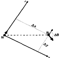
In a state-relative coordinate system these same con­ straints apply to the 0 component, but the constraints over x and y need to be specified with respect to the explicit coordinate system used. As shown in Figure 3, each state, s;, has its own coordinate system; the y axis is aligned with the robot's heading in the state (denoted by bold arrows in the figure), and the x axis is perpen­ dicular to it. The geomettic relation from s; to s i is expressed with respect to the coordinate system of s;.

Given a pair of states a and b, we denote by p(x,y) (a, b) the vector (p(Ra , b[x]), p(Ra,b[y])). Let us define Tab

. Figure 3: Robot in stateS;, faces in the y-axis direction; the relationS; ,Sj is WRT S; 's coordinate system .

to be the transformation that maps an (xa, Y a) point rep­ resented with respect to the coordinate system of state a, to the same point represented with respect to the co­ ordinate system of state b, (xb, Y b) ·

More explicitly, let Jl� b be, as before, the mean change in heading from state a to state b. Applying Tab to a vector (x·) results in the vector ( x,) as follows: Ya Yo

The consistency constraints are then restated as follows (and referred to as relative constraints from here on):

The following sections describe the learning algorithm and the initialization procedure. For clarity and brevity, proofs and a lot of technical detail are omitted, and we concen­ trate on enforcing the global constraints rather than the rel­ ative ones. The extension is straightforward, and the results reported in Section 6 were indeed obtained under relative coordinate systems. The complete proofs, treatment of the relative constraints, extension to complete POMDPs and fur­ ther results can be found in [Sha99].

4 Learning the Model

The learning algorithm starts from an initial model .>.0 and is given a sequence of experience E; it returns a re­ vised model .>., with the goal of maximizing the likelihood P(Ei.>.). The experience sequence E is of length T; each element, E,, is a pair ( r,, vt), where r, is the observed re­ lation vector along the x, y and 0 dimensions, between the states q, _1 and q, and vt is the observation vector at time t. Our algorithm extends the Baum-Welch algorithm [Rab89] to deal with the relational information and the factored observation sets. The Baum-Welch algorithm is an expectation-maximization (EM) algorithm [DLR77]; it al­ ternates between

• the E-step of computing the state-occupation and state­ transition probabilities, 1 and �, at each time in the sequence given E and the current model .>., and
• theM-step of finding a new model, "X, that maximizes P(Ei>-,,,�),

providing monotone convergence of the likelihood function P(Ei.>.) to a local maximum.

三

一

However, our extension introduces an additional compo­ nent, namely, the relation (R) matrix. It can be viewed as having two kinds of observations: state observations (as the ordinary HMM -with the distinction that we observe inte­ ger vectors rather than integers) and transition observations (the odometry relations between states). The latter must satisfy geometrical constraints. Hence, an extension of the standard update formulae, as described below, is required.

4.1 State-Occupation Probabilities

Following Rabiner [Rab89], we first compute the forward (a) and backward ((3) matrices. a1 ( i ) denotes the probabil­ ity density value of observing Eo through E1 and q1 = s;, given >.; (31 ( i) is the probability density of observing E1+1 through ET _1 given q1 = s; and >..

The forward procedure for calculating the a matrix is initialized with and continued for 0 < t ::; T - 1 with

f(r1 I R i,j ) denotes the density at point r1 according to the distribution represented by the means and variances in en­ try i, j of the relation matrix R, and b{ is the probability of observing vector Vt in state Sj; that is, b{ = n:=O B;,j,v,[i]·

The backward procedure for calculating the (3 matrix is ini­ tialized with f3 T - i{ j) = 1, and continued for 0:::; t < T- 1 with N-1

Given a and (3, we now compute the state-occupation and state-transition probabilities, 1 and�. The state-occupation probabilities are computed as follows:

Similarly, the state-transition probabilities are computed as:

These are essentially the same formulae appearing in Ra­ biner's tutorial [Rab89], but they also take into account the density of the odometric relations.

In the next phase of the algorithm, the goal is to find a new model, A, that maximizes Pr(EI>., /, � ) . Usually, this is simply done using maximum-likelihood estimation of the probability distributions in A and B by computing expected transition and observation frequencies. In our model we must also compute a new relation matrix, R, under the con­ straint that it remain geometrically consistent. Through the rest of this section we use the notation v to denote a reesti­ mated value, where v denotes the current value.

4.2 Updating Transition and Observation Parameters

The A and B matrices can be straightforwardly reesti­ mated; A;,j is the expected number of transitions from s; to 2 divided by the expected number of transitions from s;; B;,j,o is the expected number of times o is observed along the ith dimension when in state s i, divided by the expected number of times of being in s i:

where I[c] is an indicator function with value I if c is true and 0 otherwise.

4.3 Updating Relations Parameters

When reestimating the relation matrix, R, the geometri­ cal constraints induce interdependencies among the opti­ mal mean estimates as well as between optimal variance estimates and mean estimates. Parameter estimation under this form of constraints is almost untreated in main-stream statistics [Bar84] and we found no previous existing solu­ tions to the estimation problem faced here. As an illustra­ tion, consider the following constrained estimation prob­ lem of 2 normal means.

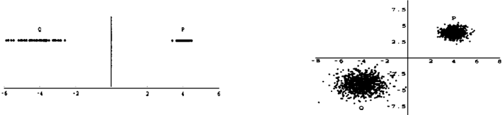
Example 1 Consider two sample sets of points P= { p 1 , P2, ... , Pn} and Q = {q1, q2, ... , qk}. inde­ pendently drawn from two distinct normal distributions with means Jlp, JlQ and variances ,. �, "'�· respectively. We are asked to find maximum likelihood estimates for the two distribution parameters. Moreover, we are told that the means of the two distributions are related, such that JJQ = -JJP, as illustrated in Figure 4. If not for the latter constraint, the task is simple [DeG86], and we have:

and similarly for JJQ and cr�. However, the constraint JJP = -JJQ requires finding a single mean J1 and setting the other one to its negated value, -jl. Intuitively, when choos­ ing such a maximum likelihood single mean, the more con­ centrated sample should have more effect while the more varied sample should be more "submissive". Thus, the overall sample deviation from the means would be mini­ mized and the likelihood of the data - maximized. There­ fore, there exists mutual dependence between the estima­ tion of the mean and the estimation of the variance.

Since the samples are independently drawn, by taking the derivatives of their joint log-likelihood function, with re­ spect to Jlp, O'p and "'Q· and equating them to 0, while using the constraint JlQ = -jlp, we obtain the following set of mutual equations for maximum likelihood estimators:

By substituting the expressions for IT p and IT Q into the ex­ pression/or J.l.p, we obtain a cubic equation which is cum­ bersome, but still solvable (in this simple case). The solu­ tion provides a maximum likelihood estimate for the mean and variance under the constraint J.l.Q = J.l.P. o

-We now proceed to the actual update of the relation matrix under constraints. For clarity, we initially discuss only the first two geometrical constraints, and discuss the additivity constraint in Section 4.4. Recall that we concentrate here on the global constraints enforcement, although the same idea is applied for the state-relative constraints.

Zero distances between states and themselves are trivially enforced, by setting all the diagonal entries in the R matrix to 0, with a small variance.

Anti-symmetry within a global coordinate system is en­ forced by using the data recorded along the transition from Sj to s; as well as from s; to Sj when reestimating J.l. ( Ri,j ) · As shown in Example 1, the variance has to be taken into account, leading to the following set of mutual equations:

For the x and y dimensions this amounts to a complicated but still solvable cubic equation. However, in the more gen­ eral case, when accounting for the orientation of the robot, and also when complete additivity is enforced, we do not obtain such closed form reestimation formulae.

To avoid these reestimation hardships, we use a lag-behind update rule; the yet-unupdated estimate of the variance is used for calculating a new estimate for the mean, and this new mean estimate is used to update the variance, using Eq. 2. 2 Thus, the mean is updated using a variance pa­ rameter that lags behind it in the update process, and the reestimation formula 1 needs to use �Ti,j rather than O'?,'j:

This lag-behind policy is an instance of generalized EM [Sha99], which guarantees monotone convergence to a local maximum of the likelihood function.

2 A similar approach, termed one step late update, is taken by others applying EM to highly non-linear optimization prob­ lems [MK97].

Similarly, the reestimation formula for the von Mises mean and concentration parameters of the heading change be­ tween states s; and s i is the solution to the equations:

..

..

Again, to avoid the need to solve these mutual equations, we take advantage of the "lag-behind" strategy, updating the mean using the current estimates of the concentration parameters, K;,j, Kj,i· as follows:

and then calculating the new concentration parameters based on the newly updated mean, as the solution to equa­ tion 4, through the use of lookup-tables.

A possible alternative to our lag-behind approach is to up­ date the mean as though the assumption ITj,i = ITi,j holds. Under this assumption, the variance terms in equation I cancel out, and the mean update is independent of the variance once again. Then the variances are updated as stated in equation 2, without assuming any constraints over them. This approach was taken in earlier stages of this work [SK97, SK98]. The lag-behind strategy is superior, both according to our experiments, and due to its being an instance of generalized EM.

4.4 Enforcing Additivity

Note that the additivity constraint implies the other two ge­ ometrical constraints, thus enforcing it results in complete geometrical consistency. One way to enforce additivity is by using the iterative anti-symmetric update procedure de­ scribed above, augmenting each iteration with a procedure for deriving an additive model from the anti -symmetric one. Our experience with such a technique proved unsatis­ factory, typically converging to poor models or altogether failing to converge.

We briefly describe here the method for directly enforcing additivity through the reestimation procedure. As before, we restrict the discussion to global coordinate systems.

二

一

4.4.1 Additivity in the x, y dimensions

The main observation underlying our approach is that the additivity constraint is a result of the fact that states can be embedded in a geometrical space. That is, assuming we have N states, s0, ... , sN_1, there ·are points on the X, Y and 0 axes, xo, ... , XN-1· yo, ... , YN-1· IJo, ... , IJN-1> respectively, such that each state, s;, is associated with the coordinates (x;, y;, 0;). Assuming one global coordinate system, the mean odometric relation from state s; to state Sj can be expressed as: (xj- x;, YJ- y;, e, -IJ;).

During the maximization phase of the EM iteration, rather than try to maximize with respect to N2 odometric relation vectors, (J.l f§ , J.l'0· J.lf j ), we reparameterize the problem. Specifically, we express each odometric relation as a func­ tion of two of the N state positions, and maximize with re­ spect to the unconstrained, N state positions. For instance, for the X dimension, we find during the maximization step N !-dimensional points, xo, ... ,XN-1. from which we calculate J.l[ j = xi - x;. Moreover, since all we are inter­ ested in is finding the best relationships between x; and xi, we can fix one of the x;'s at 0 (e.g. x0 = 0), and only find optimal estimates for the other N-1 state positions. The variance reestimation remains as before, and the lag-behind policy is used to eliminate the interdependency between the update of the mean and the variance parameters.

4.4.2 Additive Heading Estimation

Unfortunately, the reparameterization described above is not feasible for heading change estimation, due to the von Mises distribution assumption over the heading measures; By reparameterizing J.lf i as OJ -0; and maximizing the likelihood function with respect to the O's, we obtain a set of N 1 trigonometric equations with terms of the form c os ( O J) · sin ( li; ) which do not enable simple solution.

A possible alternative is to use the anti-symmetric reestimation procedure, followed by a perpendicu­ lar projection operator, mapping the headings vector (J.l g o, .. . ,J.lfj, .. . ,J.l 1v-1, N _1 ) , 0 � i,j � N-1, which does not satisfy additivity, onto a vector of headings within an additive linear vector space. Simple orthogonal pro­ jection is not satisfactory within our setting, since it sim­ ply looks for the additive vector closest to the non-additive one, ignoring the fact that some of the entries in the non­ additive vector are based on a lot of observations, while others are based on hardly any data at all. Intuitively, we would like to keep the estimates that are well accounted for intact, and adapt the less accounted for estimates in order to meet the additivity constraint. More precisely, we would like to project the non-additive heading estimates vector onto a subspace of the additive vector space, in which the vectors have the same values as the non-additive vector in the entries that are well-accounted for. The culprit is that the latter subspace is not a linear vector space (for instance, it does not satisfy closure under scalar multiplication), and the projection operator over linear spaces can not be ap-

plied directly. Still, this set of vectors does form an affine vector space, and we can project onto it using a special technique from linear algebra, as explained below 3·

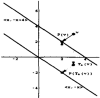
Definition A c nn is an n-dimensional affine space if for all vectors Va E A, the set of vectors: A-Va� {ua- v.lua E A} is a linear space.

Hence, we can pick a vector, v01 E A, and define the translation Ta : A -t V, where V is a linear space, V = A - v01· This translation is trivially extended for any vector v' E 7?.", by defining T.(v') = v'-va,· In order to project a vector v E Rn onto A, we apply the translation Ta to v and project Ta ( v) onto V, which results in a vector P(T.(v)) in V. By applying the inverse transform T ;; 1 to it, we obtain the projection of v on A, as demonstrated in Figure 5. The linear space in the figure is the two dimen­ sional vector space { ( x , y) I y = -x } , and the affine space is { (x, y) l y = -x + 4}. The transform Ta consists of subtracting the vector (0, 4). The solid arrow corresponds to the direct projection of the vector v onto the point P ( v) of the affine space. The dotted arrows represent the projec­ tion via translation of v to Ta ( v ) , the projection of the latter onto the linear vector space, and the inverse translation of the result, P(Ta ( v) ) , onto the affine space.

Although the procedure for preserving additivity over headings is not proven to preserve monotone convergence of the likelihood function towards a local maximum, our extensive experiments consisting of hundreds of runs have shown that monotone convergence is preserved.

5 Choosing an Initial Model

Typically, in instances of the Baum-Welch algorithm, an initial model is picked uniformly at random from the space of all possible models, perhaps trying multiple initial mod­ els to find different local likelihood maxima. An alternative approach we have reported [SK97] was based on clustering the accumulated odometric information using the simple k­ means algorithm [DH73], taking the clusters to be the states in which the observations were recorded, to obtain state and observation counts and estimate the model parameters.

When perpendicularity is assumed, as shown in Figure I, the k-means algorithm assigns the same cluster (state) to odometric readings recorded at close locations, leading to reasonable initial models. However, when this assump-

3Many thanks to John Hughes for introducing this technique.

tion is dropped, as illustrated in Figure 2, the cumulative rotational error distorts the odometric location recorded within a global coordinate system, so that the location as­ signed to the same state during multiple visits varies greatly and would not be recognized as "the same" by a simple location-based clustering algorithm. To overcome this, we developed an alternative initialization heuristics, based di­ rectly on the recorded relations between states- rather than on absolute states location. For clarity, the description here is informal, consisting mostly of an illustrative example, and enforcing global consistency constraints.

Given a sequence of observations and odometric readings E, we begin by clustering the odometric readings into buck­ ets. The number of buckets is at most the number of distinct state transitions recorded in the sequence. The goal at this stage is to have each bucket contain all the odometric read­ ings that are close to each other along all three dimensions.

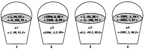
To achieve this, we start by fixing a predetermined, small standard deviation value along the x, y, and (J dimensions. Denote these standard deviation values O'x, O'y, 0'9 respec­ tively, (typically 0' x = 0' y ) . The first odometric reading is assigned to bucket 0 and the mean of this bucket is set to be the value of this reading. Through the rest of the process the subsequent odometric readings are examined. If the next reading is within 1.5 standard deviations along each of the three dimensions from the mean of some ex­ isting non-empty bucket, add it to the bucket and update the bucket mean accordingly. If not, assign it to an empty bucket and set the mean of the bucket to be this reading.

This algorithm guarantees that all the odometric readings in each bucket are within a range of 1.5· ( 0' x· O'y, 0'9 ) from the bucket mean. Since the actual sample standard deviation of each bucket can not exceed the fixed deviation used dur­ ing the bucketing process, intuitively, each bucket is tightly concentrated about its mean. We note that other clustering algorithms [DH73] could be used at the bucketing stage.

Example 2 We would like to learn a 4-state model from a sequence whose odometric component is as follows:

As a first stage we place these readings into buckets. Sup­ pose the standard deviation constant is 20. The placement is as shown in Figure 6. The mean value associated with each bucket is shown as well. o

The next stage of the algorithm is the state-tagging phase, in which each odometric reading, r,, is assigned a pair of states, s;, Sj, denoting the origin state (from which the tran­ sition took place) and the destination state (to which the transition led), respectively. In conjunction, the mean en­ tries, J.Lii, of the relation matrix, R, are populated.

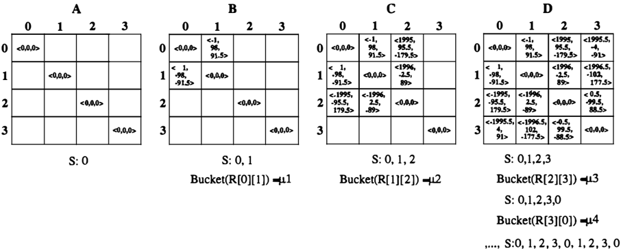
Example 2 (cont.) Returning to the sequence above, the process is demonstrated in Figure 7. We assume that the data recording starts at state 0, and that the odometric change through self transitions is 0, with some small stan­ dard deviation (we use 20 here as well). This is shown on part A of the figure.

Since the first element in the sequence, (2 94 92), is more than two standard deviations away from the mean p.(O][OJ and no other entry in the relation row of state 0 is popu­ lated, we pick 1 as the next state and populate the mean p.[O][l] to be the same as the mean of bucket 1, to which (2 94 92) belongs. To maintain geometrical consistency the mean p.[1][0] is set to be -p.[0][1], as shown in part B of the figure. We now have populated 2 off-diagonal entries, and the state sequence is (0, 1 ) . The entry (OJ [1] in the ma­ trix becomes associated with bucket 1, and this information is recorded for helping with tagging future odometric read­ ings belonging to the same bucket.

The next odometric reading, (1994 0 88), is a few standard deviations from any populated mean in row 1 (where 1 is the current believed state). Hence, we pick a new state 2, and set the mean p.[1][2] to be p.2-the mean of bucket 2to which the reading belongs (Figure 7 C). The entry [1][2] is recorded as associated with bucket 2. To preserve anti­ symmetry and additivity, p.[2][1] is set to -p.[l](2]. p.[0](2] is set to be the sum p.(0][1] + p.(1][2], and p.(2][0] is set to -p.(0][2]. Similarly, p.(2][3] is updated to be the mean of bucket 3, causing the setting of p.(3][2], p.(1][3], r(0][3], p.(3](1], and r(3](0]. Bucket 3 is associated with r(2][3].

At this stage the odometric table is fully populated, as shown in part D of Figure 7. The state sequence at this point is: (0, 1, 2, 3). The next reading, (-1999 -1 94), is within one standard deviation from p.(3] (0] and therefore the next state is 0. Entry (3][0] is associated with bucket 4, (the bucket to which the reading was assigned), and the state sequence becomes: (0, 1, 2, 3, 0).

The next reading, being from bucket 1, is associated with the relation from state 0 that is tagged by bucket 1, namely, state 1. By repeating this for the last two readings, the final state transition sequence becomes (0, 1, 2, 3, 0, 1, 2, 3, 0). 0

Once the state-transition sequence is obtained, the rest of the initialization algorithm is the same as it is for k­ means based initialization, deriving state-transition counts from the state-transition sequence, assigning the observa­ tions to the states under the assumption that the state se­ quence is correct, and obtaining state-transition and obser­ vation probabilities. The initialization phase does not incur much computational overhead, and is equivalent time-wise to performing one additional iteration of the EM procedure.

二

L

Figure 7: Populating the odometric relation matrix and creating a state tagging sequence.

6 Experiments and Results

Our experiments consist of learning models from both real and simulated robot data (without assuming perpendicular­ ity), evaluating the results both visually and statistically.

6.1 Experimental Setting

We ran our robot, Ramona, along a prescribed 4 directed path in the Brown CS department. Low-level routines let Ramona move forward from one hallway intersection to the next and to turn 90° to the left or right. Ultrasonic data in­ terpretation lets her perceive, in three directions- front, left and right - whether there is an open space, a door, a wall, or something unknown. Doors and intersections constitute states. When they are detected, Ramona stops and records its observations, and its odometric change between the pre­ vious and the current state. All recorded measures as well as the actions are, of course, subject to error.

The path Ramona followed consists of 4 connected corri­ dors, including 17 states, and is shown as an HMM in Fig­ ure 8. Black dots represent the physical locations of states. Multiple states (shown as numbers in the plot) associated with a single location correspond to different orientations of the robot at that location. The larger circle, at the bot­ tom left comer, represents the initial position. Solid arrows represent the most likely directed transition (corridor tra­ versed) between states and dashed arrows represent transi­ tions that have probability 0.2 or higher (if such exist). The arrow length represents the corridor length, drawn to scale. The observations associated with each state are omitted for clarity. A projection of the odometric readings recorded along the x and y dimensions, was shown in Figure 2.

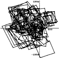
To statistically evaluate our algorithm, we use a simulated office environment in which the robot follows a prescribed path. It is represented as an HMM consisting of 44 states, and the associated transition, observation, and odometric distributions. Figure 11 depicts this HMM. We generated 5 data sequences from the model, each of length 800, us­ ing Monte Carlo sampling. One of these sequences is de-

4Hence, no decisions are executed by the robot, and the model is an HMM and not a complete POMDP.

picted in Figure 12. Again, observations are omitted, and this is a projection of the odometry readings onto a global 2-dimensional coordinate system. For each sequence we ran our algorithm 10 times. For comparison, we also ran the standard Baum-Welch algorithm, not using odometric information, 10 times on each sequence.

6.2 Results

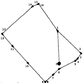
We used our algorithm, enforcing additivity and using the initialization procedure of Section 5, to learn a model of the environment from the data gathered by Ramona. Figure 9 depicts a typical model learned from that data; the learned R matrix was used for determining relative state positions. It is clear that the model corresponds well both topologi­ cally and geometrically to the true environment. The ob­ servation distributions learned are omitted, but they too re­ flect well the walls, doors and openings encountered, while incorporating the identification error resulting from noisy sensors. Note that the initial state, 0, is not well positioned geometrically with respect to the rest of the model; due to the large number of states neighboring the initial state, 0, in the true environment, it was not recognized that we ever returned to this particular state during the loop. Therefore, only one expected transition was recognized from state 0 to state 1 by the algorithm. When projecting the angles to maintain additivity, the angle from state 0 to 1 was conse­ quently compromised, maintaining the rectangular geome­ try among the more regularly visited states.

Note that learning such circular topologies is very challeng­ ing, since their highly symmetric nature makes it difficult to distinguish separate states, as well as to identify when the same state is revisited; as far as we know no other topo­ logical approach can learn such models from raw data, and the only other work which handles them is the grid-based geometrical approach of Thrun et a! [TBF98].

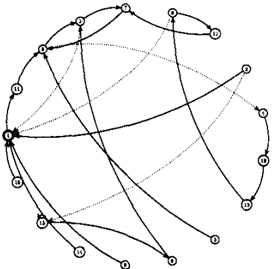
Figure 10 shows the topology of a typical HMM learned us­ ing the standard Baum-Welch algorithm without odomet­ ric information. The bold circle represents the initial state. The arrows semantics is as before. The loop topology of the traversed environment is obviously not captured.

· Figure ' 8� ' -T rue model of the �� rridors Ramona traversed.

Figure 12: A data sequence generated from the simulated model

Traditionally, in simulation experiments, learned models are quantitatively compared to the actual model that gener­ ated the data. Each of the models induces a probability dis­ tribution on strings of observations; the Kullback-Leibler divergence [KL51] between the two distributions is a mea­ sure of how far the learned model is from the true model. We report our simulation results in terms of a sampled ver­ sion of the KL divergence, as described by Juang and Ra­ biner [JR85]. It is based on generating sequences of suf­ ficient length according to the distribution induced by the true model, and comparing their likelihoods according to the learned model, with the true model likelihoods. Ode­ metric information is ignored when applying the KL mea­ sure, thus allowing comparison between purely topological models that are learned with and without odometry.

Table 1 lists the KL divergence between the true and learned model, as well as the number of iterations until conver­ gence was reached, for each of the 5 simulation sequences under the two learning settings, averaged over 10 runs per sequence. The table demonstrates that the KL divergence with respect to the true model for models learned using odometric data, is about 8 times sTIUiller than for models learned without it. To check the significance of our results we used the simple two-sample t-test. The models learned using odometric information have highly statistically sig­ nificantly (p « 0.0005) lower average KL divergence than the others. In addition, the number of iterations required for convergence when learning using odometric informa­ tion is smaller than required when ignoring such informa­ tion. Again, the t-test verifies the significance (p < 0.005) of this result.

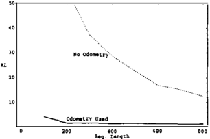
Learning HMMs obviously requires visiting states and tran-

sitioning between them multiple times, to gather sufficient data for robust statistical modeling. Intuitively, exploiting odometric data can help reduce the number of visits needed for obtaining a reliable model. To examine the influence of reduction in the length of data sequences on the quality of the learned models, we took one of the 5 sequences and used its prefixes of length 100 to 800 (the complete se­ quence), in increments of 100, as training sequences. We ran the two algorithmic settings over each of the 8 prefix sequences, 10 times repeatedly. The KL divergence was then used to evaluate each resulting model with respect to the true model. For each prefix length we averaged the KL divergence over the 10 runs. Figure 13 depicts the av­ erage KL divergence as a function of the sequence length for each of the settings. It demonstrates that , in terms of the KL divergence, our algorithm, using odometric infor­ mation, is robust in the face of data reduction, (down to 200 data points). In contrast, learning without the use of odom­ etry quickly deteriorates as the amount of data is reduced.

7 Conclusions

Odometric information, which is often readily available in the robotics domain, makes it possible to learn hidden Markov models efficiently and effectively, while using shorter training sequences. The odometric information can be directly incorporated into the traditional HMM model, maintaining convergence of the reestimation algorithm to a local maximum of the likelihood function.

Even though we are primarily interested in the underly­ ing topological model (transition and observation proba­ bilities), our experiments demonstrate that using odomet­ ric relations can both reduce the number of iterations re­ quired by the algorithm and improve the resulting model.

一

---;

Table 1: Average results of 2 learning settings with 5 training sequences.

Seq. #		I	2	3	4	5
With	KL	1.46	1.18	1.20	1. 02	1.22
Odo	Iter#	1 1.8	36.8	30.7	24.6	33.3
No	KL	6.91	9.93	1 0.03	9.54	12.43
Odo	Iter#	1 13.3	1 13.1	1 02.0	1 04.2	1 12.5

The initialization proced\U'e and the enforcement of the ad­ ditivity constraint over relatively small models prove help­ ful both topologically and geometrically. An extensive study [Sha99] shows that for long data sequences, gen­ erated from large models, enforcing only anti-symmetry rather than additivity, leads to better topological models. This is because in these cases, initialization is not always good, and additivity may over-constrain the learning to an unfavorable area. Learning of large models may benefit from enforcing only anti-symmetry dW"ing the first few it­ erations, and complete additivity in later iterations. Alter­ natively, we may use our algorithm to learn separate mod­ els for small portions of the environment, combining them later into one complete model.

The work presented here demonstrates how domain­ specific information and constraints can be incorporated into the statistical estimation process, resulting in better models, while requiring shorter data sequences. We strongly believe that this idea can be applied in domains other than robotics. In particular, the acquisition of HMMs for use in Molecular Biology may greatly benefit from exploiting geometrical (and other) constraints on molecu­ lar structures. Similarly, temporal constraints may be ex­ ploited in domains in which POMDPs are appropriate for decision-support, such as air-traffic control and medicine.

Acknowledgments

I am grateful to Leslie Kaelbling for her guidance throughout this work, and particularly for suggesting the bucketing phase, Se­ bastian Thrun for his insightful comments, John Hughes for the affine projection technique, Jim Kurien for the low level robot software and Bill Smart for maintaining Ramona.

References

• [Asa91] M. Asada, Map Building for a Mobile Robot from Sen­ sory Data, Autonoi'IWUS Mobile Robots, S. S. Iyengar and A. Elfes, eds., pp. 312-322, IEEE Press, 1991.
• [Bar84] R. Bartels, Estimation in a Bidirectional Mixture of von Mises Distributions, Biometrics, 40, pp. 777-784, 1984.
• [CKK96] A. R. Cassandra, L. P. Kaelbling and J. A. Kurien, Act­ ing Under Uncertainty: Discrete Bayesian Models for Mobile-Robot Navigation, Proc. of the Int. Con f. on In­ telligent Robots and Systems, 1996.
• [DeG86] M. H. DeGroot, Probability and Statistics, Addison­ Wesley, 2nd edn., 1986.
• [DH73] R. 0. Duda and P. E. Hart, Pattern Classi fication and Scene Analysis, chap. 6, John Wiley and Sons, 1973.
• [DLR77] A. P . Dempster, N. M. Laird and D. B. Rubin, Max­ imum Likelihood from Incomplete Data via the EM Algorithm, Journal of the Royal Statistical Society, 39 (1 ), pp. 1-38, 1977 0
• [GGD53] E. G. Gumbel, J. A. Greenwood and D. Durand, The Circular Normal Distribution: Theory and Tables, American Statistical Society Journal, 48, pp. 131-152, 1953.
• [GJ97] Z. Ghahramani and M. I. Jordan, Factorial Hidden Markov Models, Proc. of the Int. Con f. on Machine Learning, 1997.
• [HG95] D. Heckerman and D. Geiger, Learning Bayesian Net­ works: A Unification for Discrete and Gaussian Do­ mains, Proc. of the Int. Con f. on Uncertainty in AI, pp. 27 4-284, 1995 0
• [JR85] B. H. Juang and L. R. Rabiner, A Probabilistic Distance Measure for Hidden Markov Models, AT&T Technical Journal, 64 (2), pp. 391-408, 1985.
• [KB91] B. Kuipers and Y.-T. Byun, A Robot Exploration and Mapping Strategy Based on a Semantic Hierarchy of Spatial Representations, Journal o f Robotics and Au­ tonoi'IWUS Systems, 8, pp. 47-63, 1991.
• [KL51] S. Kullback and R. A. Leibler, On Information and Sufficiency, Annals of Mathematical Statistics, 22 (1), pp. 79--86, 195 1.
• [KS96a] S. Koenig and R. G. Simmons, Passive Distance Learn­ ing for Robot Navigation, Proc. of the Int. Conf. on Machine Learning, pp. 266--274, 1996.
• [KS96b] S. Koenig and R. G. Simmons, Unsupervised Learning of Probabilistic Models for Robot Navigation, Proc. o f the Int. Con f. on Robotics and Automation, 1996.
• [Mar72] K. V. Mardia, Statistics o f Directional Data, Academic Press, 1972.
• [ME85] H. P. Moravec and A. Elfes, High Resolution Maps from Wide Angle Sonar, Proc. o f the Int. Con f. on Robotics and Automation, pp. 1 16--121, 1985.
• [MK97] G. J. McLachlan and T. Krishnan, The EM Algorithm and Extensions, John Wiley & Sons, 1997.
• [NPB95] I. Nourbakhsh, R. Powers and S. Birchfield, DERVISH: An Office-Navigating Robot, A/ Magazine, 16 ( 1 ), pp. 53-60, 1995.
• [Rab89] L. R. Rabiner, A Tutorial on Hidden Markov Mod­ els and Selected Applications in Speech Recognition, Proc. o f the I E E E, 77 (2), pp. 257-285, 1989.
• [Sha99] H. Shatkay, Learning Models f or Robot Navigation, Ph.D. thesis, Tech. Rep. CS-98-1 1, Dept. of Computer Science, Brown University, Providence, Rl, 1999.
• [SK95] R. G. Simmons and S. Koenig, Probabilistic Naviga­ tion in Partially Observable Environments, in Proc. o f the Int. Joint Conf. on Artificial Intelligence, 1995.
• [SK97] H. Shatkay and L. P . Kaelbling, Learning Topologi­ cal Maps with Weak Local Odometric Information, in Proc. o f the Int. Joint Con f. on Artificial Intelligence, 1997.
• [SK98] H. Shatkay and L. P . Kaelbling, Heading in the Right Direction, in Proc. o f the Int. Con f. on Machine Learn­ ing, 1998.
• [SSC9l] R. Smith, M. Self and P. Cheeseman, A Stochstic Map for Uncertain Spatial Relationships, in Autonoi'IWus Mobile Robots, S. S. Iyengar and A. Elfes, eds., pp. 323-330, IEEE Computer Society Press, 1991.
• [fBF98] S. Thrun, W. Burgard and D. Fox, A Probabilistic Ap­ proach to Concurrent Map Acquisition and Localiza­ tion for Mobile Robots, Machine Learning, 31, pp. 2953, 1998.