Logic Programming with Social Features ∗

FRANCESCO BUCCAFURRI and GIANLUCA CAMINITI

DIMET - Universit` a 'Mediterranea' degli Studi di Reggio Calabria via Graziella, loc. Feo di Vito, 89122 Reggio Calabria, Italia ( e-mail: [email protected], [email protected] )

submitted 16 January 2007 ; revised 13 November 2007, 18 April 2008; accepted 21 May 2008

Abstract

In everyday life it happens that a person has to reason about what other people think and how they behave, in order to achieve his goals. In other words, an individual may be required to adapt his behaviour by reasoning about the others' mental state. In this paper we focus on a knowledge representation language derived from logic programming which both supports the representation of mental states of individual communities and provides each with the capability of reasoning about others' mental states and acting accordingly. The proposed semantics is shown to be translatable into stable model semantics of logic programs with aggregates. To appear in Theory and Practice of Logic Programming (TPLP).

KEYWORDS : logic programming, stable model semantics, knowledge representation

1 Introduction

In everyday life it happens that a person has to reason about what other people think and how they behave, in order to achieve his goals. In other words, an individual may be required to adapt his behaviour by reasoning about the others' mental state. This typically happens in the context of cooperation and negotiation: for instance, an individual can propose his own goals if he knows that they would be acceptable to the others. Otherwise he can decide not to make them public. As a consequence, one can increase the success chances of his actions, by having information about the other individuals' knowledge.

In this paper we focus on a knowledge representation language derived from logic programming which both supports the representation of mental states of individual communities and provides each with the capability of reasoning about others' mental states and acting accordingly. The proposed semantics is shown to be translatable into stable model semantics of logic programs with aggregates.

We give the flavor of the proposal by two introductory examples, wherein we describe the features of our approach in an informal, yet deep fashion. Even though in these examples, as well as elsewhere in the paper, we use the term agent to denote

∗ An abridged version of this paper appears in (Buccafurri and Caminiti 2005).

the individual reasoning, we remark that our focus is basically concerning to the knowledge-representation aspects, with no intention to investigate how this reasoning layer could be exploited in the intelligent-agent contexts. However, in Section 8, we relate our work with some conceptual aspects belonging to this research field.

Consider now the first example.

Example 1

There are four agents which have been invited to the same wedding party. These are the desires of the agents:

• Agent 1 will go to the party only if at least the half of the total number of agents (not including himself) goes there.
• Agent 2 possibly does not go to the party, but he tolerates such an option. In case he goes, then he possibly drives the car.
• Agent 3 would like to join the party together with Agent 2 , but he does not trust on Agent 2 's driving skill. As a consequence, he decides to go to the party only if Agent 2 both goes there and does not want to drive the car.
• Agent 4 does not go to the party.

Now, assume that some agents are less autonomous than the others, i.e. they may decide either to join the party or not to go at all, possibly depending on the other agents' choice. Moreover some agents may not require, yet tolerate some options.

The standard approach to representing communities by means of logic-based agents (Satoh and Yamamoto 2002; Costantini and Tocchio 2002; De Vos et al. 2005; Alberti et al. 2004; Subrahmanian et al. 2000) is founded on suitable extensions of logic programming with negation as failure ( not ) where each agent is represented by a single program whose intended models (under a suitable semantics) are the agent's desires/requests. Although we take this as a starting point, it is still not suitable to model the above example because of two following issues:

1. There is no natural representation for tolerated options, i.e. options which are not requested, but possibly accepted (see Agent 2 ).
2. Amachinery is missing which enables one agent to reason about the behaviour of other agents (see Agent 1 and Agent 3 ).

In order to solve the first issue (item 1.) we use an extension of standard logic programming exploiting the special predicate okay (), previously introduced in (Buccafurri and Gottlob 2002). Therein a model-theoretic semantics aimed to represent a common agreement in a community of agents was given. However, representing the requests/acceptances of single agents in a community is not enough. Concerning item 2 above, a social language should also provide a machinery to model possible interference among agents' reasoning (in fact it is just such an interference that distinguishes the social reasoning from the individual one). To this aim, we introduce a new construct providing one agent with the ability to reason about other agents' mental state and then to act accordingly.

Program rules have the form:

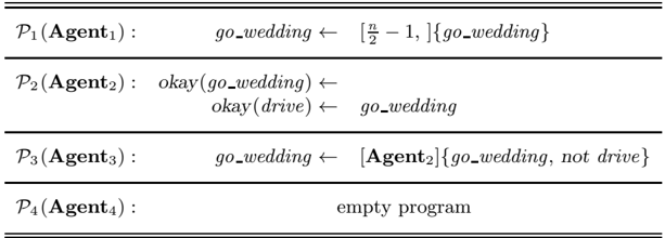
P 1 ( Agent 1 ) :	go wedding ←	[ n 2 - 1, ] { go wedding }
P 2 ( Agent 2 ) :	okay ( go wedding ) ← okay ( drive ) ←	go wedding
P 3 ( Agent 3 ) :	go wedding ←	[ Agent 2 ] { go wedding , not drive }
P 4 ( Agent 4 ) :	empty program

where selection condition predicates about some social condition concerning either the cardinality of communities or particular individuals satisfying body .

For instance, consider the following rule, belonging to a program representing a given agent A :

This rule means that agent A will require a in case a number ν of agents (other than A ) exists such that they require or tolerate b , neither require nor tolerate c and it holds that 0 ≤ l ≤ ν ≤ h ≤ n -1. By default, l = 0 and h = n -1. The number n is a parameter - known by each agent - representing the total number of agents (including the agent A ). This enriched language is referred to as SOcial Logic Programming (SOLP). The wedding party scenario of Example 1 can be represented by the four SOLP programs shown in Table 1, where the program P 4 is empty since the corresponding agent has not any request or desire to express.

The intended models represent the mental states of each agent inside the community. Concerning the party, such models are the following:

M 1 = ∅ , M 2 = { go wedding P 1 , go wedding P 2 , drive P 2 } , and M 3 = { go wedding P 1 , go wedding P 2 , go wedding P 3 } , where the subscript P i (1 ≤ i ≤ n ) references, for each atom in a model, the program (resp. agent) that atom is entailed by. The models respectively mean that either ( M 1 ) no agent will go to the party, ( M 2 ) only Agent 1 and Agent 2 will go and also Agent 2 will drive the car, or ( M 3 ) all agents but Agent 4 will go to the party.

Let us show why the above models represent the intended meaning of the program: M 1 is empty in case Agent 2 does not go to the wedding party (i.e. go wedding is not derived by P 2 ). Indeed, in such a case, Agent 3 will not go too, since his requirements w.r.t. Agent 2 are not satisfied. Moreover, since Agent 4 expresses neither requirements nor tolerated options, he does not go to the party (observe that such a behaviour is also represented by the models M 2 and M 3 ). Finally, Agent 1 requires that at least one 1 agent (other than himself) goes to the party. As a consequence of the other agents' behaviour, Agent 1 will not go. Thus, no agent will go to the party and M 1 is empty. The intended meaning of M 2 is that both Agent 1

1 Since n 2 -1 = 1, where n is the total number of agents, i.e. n =4.

and Agent 2 will go to the party and Agent 2 will also drive the car. In such a case Agent 3 will not go since he requires that Agent 2 does not drive the car. The model M 3 represents the case in which Agent 2 goes to the party, but does not drive the car. Now, since all requirements of Agent 3 are satisfied, then he also will go to the party. Certainly, Agent 1 will join the other agents, because, in order to go to the party, he requires that at least one agent goes there.

The intended models are referred to as social models , since they express the results of the interactions among agents. As it will be analyzed in Section 6, the multiplicity of intended models is induced both by negation occurring in rule bodies and also directly by the social features, thus making the approach non-trivial.

Let us informally introduce the most important properties of the semantics of the language:

• Social conditions model reasoning conditioned by the behaviour of other agents in the community. In particular, it is possible to represent collective mental states, preserving the possibility of identifying the behaviour of each agent.
• It is possible to nest social conditions, in order to apply recursively the socialconditioned reasoning to agents' subsets of the community.
• Each social model represents the mental state (i.e. desires, requirements, etc.) of every agent in case the social conditions imposed by the agents are enabled.

Observe that, in order to meet such goals, merging all the input SOLP programs it is not enough, since this way we lose all information about the relationship between an atom and the program (resp. agent) which such an atom comes from. Therefore, we have to find a non-trivial solution.

Our approach starts from (Buccafurri and Gottlob 2002), where the Joint Fixpoint Semantics (JFP), that is a semantics providing a way to reach a compromise (in terms of a common agreement) among agents modelled by logic programs, is proposed. Therein, each model contains atoms representing items being common to all the agents. The approach proposed here in order to reach a social-based conclusion is more general: the agents' behaviour is defined by taking into account social conditions specified by the agents themselves.

Informally, a social condition is an expression [ selection condition ] { body } , where selection condition can be of two forms: either (i) cardinality-based, or (ii) identitybased. In the former case the agent requires that a number of other agents (bounded by selection condition itself) satisfy body . In the latter case, selection condition identifies which agent is required to satisfy body . Given a program rule including a social condition such as head ← [ selection condition ] { body } , the intuitive meaning is that head is derived if the social condition is satisfied.

An example of cardinality-based condition (case (i) above) is shown in Table 1 by the program P 1 : an intended model M will include the atom go wedding P 1 if a set of programs S ′ ⊆ {P 2 , P 3 , P 4 } exists such that for each P ∈ S ′ , it results that go wedding P belongs to M and also it holds that the number of programs in S ′ satisfies the social condition imposed by the program P 1 , that is | S ′ | ≥ n 2 -1.

An example of case (ii) (identity-based condition) is represented by the program

P 3 , which requests the atom go wedding P 3 to be part of an intended model M if go wedding P 2 belongs to M , but the atom drive P 2 does not. Importantly, social conditions can be nested each other, as shown by the next example.

Example 2

Consider a Peer-to-Peer file-sharing system where a user can share his collection of files with other users on the Internet. In order to get better performance, a file is split in several parts being downloaded separately (possibly each part from a different user) 2 . The following SOLP program P describes the behaviour of an agent (acting on behalf of a given user) that wants to download every file X being shared by at least a number min of users such that at least one of them owns a complete version of X (rule r 1 ). Moreover, the agent tolerates to share any file X of his, which is shared also by at least the 33% of the total number of users in the network and such that among those users, a number of them (bounded between 20% and 70% of the total) exists having a high bandwidth. In this case the agent tolerates to share, since he is sure that the network traffic will not be unbalanced (rule r 2 ). Observe that the use of nested social conditions in P is emphasized by means of program indentation.

Now, one could argue that a different choice concerning the selection condition could be done. As a first observation we note that the chosen selection conditions play frequently an important role in common-sense reasoning. Indeed, it often happens that the beliefs and the choices of an individual depend on how many people think or act in a certain way. For instance, a person who needs a new mobile phone is interested in collecting - from his colleagues or the Internet - a number of opinions on a given model, in order to decide whether he should buy it. It occurs also that one is interested in the behaviour of a given person, in order to act or to infer something. For example, two people are doing shopping together and do not want to buy the same clothes in order not to be dressed the same way. So, one of them decides not to buy a given item, in case it has been chosen by his partner. These short examples show that two important parameters acting in the social influence are either (i) the number or (ii) the identity of the people involved. For such a reason, we propose a simple, clear-cut, yet general mechanism to represent the selection of a social condition.

As a second observation we remark that this work represents a first step towards a thorough study on how to include in a classical logic-programming setting the paradigm of social interference, in order to directly represent community-based

2 Among others, KaZaA, EMule and BitTorrent are the most popular Internet P2P file-sharing systems exploiting such a feature.

reasoning. To this aim, we focus on some suitable selection conditions, but we are aware that other possible choices might be considered. From this perspective, our work tries to give some non-trivial contributions towards what kind of features a knowledge representation language should include, in order to be oriented to complex scenarios. Anyway, as it will be shown by examples throughout the paper, the chosen social conditions combined with the power of nesting allow us to represent more articulated selections among agents.

Besides the definition of the language, of its semantics and the application to Knowledge Representation, another contribution of the paper is the translation of SOLP programs into logic programs with aggregates 3 . In particular, given a set of SOLP programs, a source-to-source transformation exists which provides as output a single logic program with aggregates whose stable models are in oneto-one correspondence with the social models of the set of SOLP programs. The translation to logic programs with aggregates give us the possibility of exploiting existing engines to compute logic programs.

Moreover, Section 6 shows that our kind of social reasoning is not trivial, since even in the case of positive programs, the semantics of SOLP has a computational complexity which is NP-complete.

The paper is organized as follows: in Sections 2 and 3 we define the notion of SOLP programs and their semantics ( Social Semantics ), respectively. In Section 4 we illustrate how a set of SOLP programs, each representing a different agent, is translated into a single logic program with aggregates whose stable models describe the mental states of the whole agent community and then we show that such a translation is sound and complete. In Section 5 we prove that the Social Semantics extends the JFP Semantics (Buccafurri and Gottlob 2002) and in Section 6 we study the complexity of several interesting decision problems. Section 7 describes how this novel approach may be used for knowledge representation by means of several examples. Then, in Section 8 we discuss related proposals and, finally, we draw our conclusions ans sketch the future directions of the work.

In order to improve the overall readability, these sections are followed by Appendix A - where we have placed the proofs of the most complicated technical results - and by the list of symbols and abbreviations used throughout the paper.

2 Syntax of SOLP Programs

In this section we first introduce the notion of social condition and then we describe the syntax of SOLP programs.

A term is either a variable or a constant. Variables are denoted by strings starting with uppercase letters, while those starting with lower case letters denote constants. An atom or positive literal is an expression p ( t 1 , · · · , t n ), where p is a predicate of arity n and t 1 , · · · , t n are terms. A negative literal is the negation as failure (NAF) not a of a given atom a .

3 As it will be shown in Section 4, we choose the syntax of the non-disjunctive fragment of DLP A (Dell'Armi et al. 2003), supported by the DLV system (Leone et al. 2002).

Definition 1

Given an integer n > 0, a ( n -) social condition s , also referred to as ( n -)SC, is an expression of the form cond ( s ) property ( s ), such that:

1. cond ( s ) is an expression [ α ] where α is either (i) a pair of integers l , h such that 0 ≤ l ≤ h ≤ n -1, or (ii) a string;
2. property ( s ) = content ( s ) ∪ skel ( s ), where content ( s ) is a non-empty set of literals and skel ( s ) is a (possibly empty) set of SCs.

n -social conditions operate over a collection of n programs representing the agent community. Each agent is modelled by a program (we will formally define later in this section which kind of programs are allowed). n represents the total number of agents. In the following, whenever the context is clear, n is omitted.

Concerning item (1) of the above definition, in case (i), cond ( s ) is referred to as cardinal selection condition , while, in case (ii), cond ( s ) is referred to as member selection condition .

Concerning item (2) of Definition 1, if skel ( s ) = ∅ then s is said simple . For a simple SC s such that content ( s ) is singleton, the enclosing braces can be omitted. Finally, given a SC s , the formula not s is referred to as the NAF of s . The following are simple SCs extracted from our initial wedding party example (see Table 1):

Example 3 [ n 2 -1, ] { go wedding } . Example 4 [ Agent 2 ] { go wedding , not drive } .

The social conditions occurring in the example regarding a Peer-to-Peer system (see Example 2) are not simple. As a further example, consider a SC s = [ l , h ] { a , b , c , [ l 1 , h 1 ] { d , [ l 2 , h 2 ] e } , [ l 3 , h 3 ] f } . Observe that s is not simple, since skel ( s ) = { [ l 1 , h 1 ] { d , [ l 2 , h 2 ] e } , [ l 3 , h 3 ] f } , moreover, content ( s ) = { a , b , c } .

Social conditions enable agents to specify requirements over either individual or groups within the agent community, by using member or cardinal selection conditions, respectively. Moreover, by nesting social conditions it is possible to declare requirements over sub-groups of agents, provided that a super-group satisfying a SC exists. In order to guarantee the correct specifications of nested social conditions, the notion of well-formed social condition is introduced next.

Given two n-SCs s and s ′ such that cond ( s ) = [ l , h ] and cond ( s ′ ) = [ l ′ , h ′ ] (0 ≤ l ≤ h ≤ n -1, 0 ≤ l ′ ≤ h ′ ≤ n -1), if h ′ ≤ h , then we write cond ( s ′ ) ⊆ cond ( s ).

A SC s is well-formed if either (i) s is simple, or (ii) s is not simple, cond ( s ) is a cardinal selection condition and ∀ s ′ ∈ skel ( s ) it holds that either (a) cond ( s ′ ) is a cardinal selection condition, s ′ is a well-formed social condition and cond ( s ′ ) ⊆ cond ( s ), or (b) cond ( s ′ ) is a member selection condition and s ′ is simple.

According to the intuitive explanation of the above definition, it results that, besides simple SCs, only non-simple SCs with cardinal selection condition are candidate to be well formed. Indeed, a non-simple SC with member selection condition requires some property on a single target agent, but no further sub-group of agents

could be specified by means of SCs possibly nested in it. Anyway, a further property is required to SCs with cardinal selection condition in order to be well-formed. In particular, given a non-simple SC s (with cardinal selection condition), all the SCs nested in s with cardinal condition must not exceed the cardinality constraints expressed by cond ( s ).

Example 5

The SC s = [1 , 8] { a , [3 , 6] { b , [ Agent 2 ] { c , d }}} is well-formed. Note that the nonsimple SCs s 1 = [ Agent 3 ] { a , [3 , 6] { b }} and s 2 = [4 , 7] { a , [3 , 9] b } are not wellformed, because cond ( s 1 ) is a member selection condition and, concerning s 2 , [3 , 9] b ∈ skel ( s 2 ) and [3 , 9] /negationslash⊆ [4 , 7].

From now on, we consider only well-formed SCs.

We introduce now the notion of rule. Our definition generalizes the notion of classical logic rule.

Definition 2

Given an integer n > 0, a ( n -) social rule r is a formula a ← b 1 ∧··· ∧ b m ∧ s 1 ∧··· ∧ s k ( m ≥ 0, k ≥ 0), where a is an atom, each b i (1 ≤ i ≤ m ) is a literal and each s j (1 ≤ j ≤ k ) is either a n -SC or the NAF of a n -SC.

Concerning the above definition, the atom a is referred to as the head of r , while the conjunction b 1 ∧··· ∧ b m ∧ s 1 ∧···∧ s k is referred to as the body of r .

In case a is of the form okay ( p ), where p is an atom, then r it is referred to as ( n -) tolerance (social) rule . In case k = 0, then a social non-tolerance rule is referred to as classical rule .

Social tolerance rules, i.e. rules with head of the form okay ( p ), encode tolerance about the occurrence of p . The rule okay ( p ) ← body differs from the rule p ← body since the latter produces the derivation of p whenever body is satisfied, thus encoding something that is required under the condition expressed by body . According to the former rule ( okay ( p ) ← body ), the truth of body does not necessarily imply p , yet its derivation is not in contrast with the intended meaning of the rule itself. In this sense, under the condition expressed by body , p is just tolerated .

Given a rule r , we denote by head ( r ) (resp. body ( r )) the head (resp. the body) of r . Moreover, r is referred to as a fact in case the body is empty, while r is referred to as an integrity constraint if the head is missing.

Example 6

An example of non-tolerance social rule is a ← b , c , [1 , 9] { b , c , not g , [1 , 4] { d }} , [ P 2 ] { d } . An example of tolerance social rule is okay ( a ) ← not b , c , [1 , 6] { a , not f , g } , not [ P 2 ] { d } .

Definition 3

A SOLP collection is a set {P 1 , · · · , P n } of SOLP programs, where each SOLP program is a set of n -social rules.

A SOLP program is positive if no NAF symbol not occurs in it. For the sake of presentation we refer, in the following sections, to ground (i.e., variable-free) SOLP programs - the extension to the general case is straightforward.

3 Semantics of SOLP programs

In this section we introduce the Social Semantics , i.e. the semantics of a collection of SOLP programs. We assume that the reader is familiar with the basic concepts of logic programming (Gelfond and Lifschitz 1991; Baral 2003).

We start by introducing the notion of interpretation for a single SOLP program. An interpretation for a ground (SOLP) 4 program P is a subset of Var ( P ), where Var ( P ) is the set of atoms appearing in P . A positive literal a (resp. a negative literal not a ) is true w.r.t. an interpretation I if a ∈ I (resp. a / ∈ I ); otherwise it is false . A rule is true w.r.t. I if its head is true or its body is false w.r.t. I .

Recall that, for each traditional logic program Q , the immediate consequence operator T Q is a function from 2 Var ( Q ) to 2 Var ( Q ) defined as follows. For each interpretation I ⊆ Var ( Q ), T Q ( I ) consists of the set of all heads of rules in Q whose bodies are true w.r.t. I . An interpretation I is a fixpoint of a logic program Q if I is a fixpoint of the associated transformation T Q , i.e., if T Q ( I ) = I .

The set of all fixpoints of Q is denoted by FP ( Q ).

Before defining the intended models of our semantics, we need some preliminary definitions.

Let P be a SOLP program. We define the autonomous reduction of P , denoted by A ( P ), the program obtained from P by removing all the SCs from the rules in P . The intuitive meaning is that in case the program P represents the social behaviour of an agent, then A ( P ) represents the behaviour of the same agent in case he decides to operate independently of the other agents.

Definition 4

Autonomous immediate consequence operator, applied to the SOLP program P Given a SOLP program P and an interpretation I ⊆ Var ( A ( P )), let TR ( A ( P )) be the set of tolerance rules in A ( P ) and Var ∗ ( A ( P )) be the set Var ( A ( P )) \{ okay ( p ) | okay ( p ) ∈ Var ( A ( P )) } ∪ { p | okay ( p ) ∈ Var ( A ( P )) } . The autonomous immediate consequence operator AT P is the function from 2 Var ∗ ( A ( P )) to 2 Var ∗ ( A ( P )) , defined as follows:

AT P ( I ) = { head ( r ) | r ∈ A ( P ) \ TR ( A ( P )) ∧ body ( r ) is true w.r.t. I } ∪ { a | head ( r ) = okay ( a ) ∧ r ∈ TR ( A ( P )) ∧ ( body ( r ) ∧ a ) is true w.r.t. I } .

Observe that AT P , when applied to an interpretation I , extends the classical immediate consequence operator T P , by collecting not only heads of non-tolerance rules whose body is true w.r.t. I , but also each atom a occurring as okay ( a ) in the head of some rule such that both a and the rule body are true w.r.t. I .

Definition 5

An interpretation I for a SOLP program P is an autonomous fixpoint of P if I is a fixpoint of the associated transformation AT P , i.e. if AT P ( I ) = I . The set of all autonomous fixpoints of P is denoted by AFP ( P ).

4 We insert SOLP into brackets since the definition is the same as for traditional logic programs.

Observe that by means of the autonomous fixpoints of a given SOLP program P we represent the mental states of the corresponding agent, assuming that every social condition in P is not taken into account.

Example 7

Consider the following SOLP program P :

okay ( a ) ← b , [1 , ] { c } b ← [2 , 4] { d }

It is easy to see that AFP ( P ) = {{ b } , { a , b }} , i.e. the interpretations I 1 = { b } and I 2 = { a , b } are the autonomous fixpoints of P , since it holds that AT P ( I 1 ) = I 1 and AT P ( I 2 ) = I 2 .

Definition 6

Given a SOLP collection C = {P 1 , · · · , P n } , let P i (1 ≤ i ≤ n ) be a SOLP program of C and L be a set of atoms. The labelled version of L w.r.t. P i , denoted by ( L ) P i is the set { a P i | a ∈ L } . Each element of ( L ) P i is referred to as a labelled atom w.r.t. P i .

Example 8

Given a SOLP program P 1 of a SOLP collection C , if L = { a , b , c } , then ( L ) P 1 = { a P 1 , b P 1 , c P 1 } , where the program identifier P 1 indicates the associated SOLP program.

Now we introduce the concept of social interpretation , devoted to representing the mental states of the collectivity described by a given SOLP collection and then we give the definition of truth for both literals and SCs w.r.t. a given social interpretation. To this aim, the classical notion of interpretation is extended by means of program identifiers introducing a link between atoms of the interpretation and programs of the SOLP collection.

Definition 7

Let C = {P 1 , · · · , P n } be a SOLP collection. A social interpretation for C is a set ¯ I = ( I 1 ) P 1 ∪ · · · ∪ ( I n ) P n , where I j is an interpretation for P j (1 ≤ j ≤ n ) and ( I j ) P j is the labelled version of I j w.r.t. P j (see Definition 6).

Example 9

Given C = {P 1 , P 2 , P 3 } , I 1 = { a , b , c } , I 2 = { a , d , e } and I 3 = { b , c , d } , where I j is an interpretation for P j (1 ≤ j ≤ 3), then ¯ I = { a P 1 , b P 1 , c P 1 , a P 2 , d P 2 , e P 2 , b P 3 , c P 3 , d P 3 } is a social interpretation for C .

We define now the notion of truth for literals, SCs and social rules, respectively. Let C = {P 1 , · · · , P n } be a SOLP collection. Given a social interpretation ¯ I for C and a positive literal a ∈ ⋃ P∈ C Var ( P ), a (resp. not a ) is true for P j (1 ≤ j ≤ n ) w.r.t. ¯ I if a P j ∈ ¯ I (resp. a P j / ∈ ¯ I ); otherwise it is false .

Because of the recursive nature of SCs, before giving the definition of truth for a SC s , we introduce a way to identify s (and also every SC nested in s ) occurring in

a given rule r of a SOLP program P . To this aim, we first define a function which returns, for a given SC, its nesting depth.

Given a SC s , we define the function depth as follows:

Given a SOLP program P , a social rule r ∈ P and an integer n ≥ 0, we define the set MSC 〈P , r , n 〉 = { s | s is a SC occurring in r ∧ depth ( s ) = n } , i.e. the set including all the SCs having a given depth n and occurring in a social rule r of a SOLP program P . Observe that, in case the parameter n is zero, then MSC 〈P , r , 0 〉 denotes the set of SCs as they appear in the rule r of P .

Example 10

Let a ← [1 , 8] { a , [3 , 6] { b , [ P 2 ] { c , d }}} , [2 , 3] { e , f } be a rule r in a SOLP program P 1 .

Then:

MSC 〈P , r , 0 〉 = { [1 , 8] { a , [3 , 6] { b , [ P 2 ] { c , d }}} , [2 , 3] { e , f } } , MSC 〈P , r , 1 〉 = { [3 , 6] { b , [ P 2 ] { c , d }} } , MSC 〈P , r , 2 〉 = { [ P 2 ] { c , d } } , MSC 〈P , r , 3 〉 = ∅ .

Given a SOLP program P , we define the set MSC P = ⋃ r ∈P MSC 〈P , r , 0 〉 . MSC P is the set of all the SCs (with depth 0) occurring in P .

Now we provide the definition of truth of a SC w.r.t. a given social interpretation and, subsequently, the definition of truth of a social rule.

Definition 8

Let C = {P 1 , · · · , P n } be a SOLP collection, C ′ ⊆ C and P j ∈ C ′ . Given a social interpretation ¯ I for C and an n -SC s ∈ MSC P j , we say that s is true for P j in C ′ w.r.t. ¯ I if it holds that either:

1. cond ( s ) = [ P k ] ∧

∃P

k

∈

C

′

| ∀

a

∈

content

1. cond ( s ) = [ l , h ] ∧

D

∃

⊆

C

′

\ {P

j

} |

a

∀

s

∀

′

∈

content

∈

(

skel

(

s

)

s

l

≤ |

)

,

∀P ∈

D

∃

′

⊆

D

(

D

s

)

,

| ≤

D

|

,

a

is true for

h

∧

a

s

′

is true for is true for

P

P

j

P

k

w.r.t. ¯

I

,

I

w.r.t. ¯

in

∧

D

′

w.r.t. ¯

where l , h are integers and P k is a SOLP program.

If C ′ = C , then we simply say that s is true for P j w.r.t. ¯ I . An n -SC not true for P j (in C ′ ) w.r.t. ¯ I is false for P j (in C ′ ) w.r.t. ¯ I .

Finally, the NAF of a n -SC s , not s , is true (resp. false ) for P j (in C ′ ) w.r.t. ¯ I if s is false (resp. true) for P j (in C ′ ) w.r.t. ¯ I .

Informally, given a SC s included in P j , s is true for P j w.r.t. a social interpretation ¯ I if a single SOLP program P k (resp. a set D of SOLP programs not including P j ) exists such that all the elements in content ( s ) are true for P k w.r.t. ¯ I (resp. for every program P ∈ D w.r.t. ¯ I , and such that every element in skel ( s ) is true for P j w.r.t. ¯ I ). Observe that the truth of property ( s ) is possibly defined recursively, since s may contain nested SCs.

I

or

,

Once the notion of truth of SCs has been defined, we are able to define the notion of truth of a social rule w.r.t. a social interpretation.

Let C be a SOLP collection and P ∈ C . Given a social interpretation ¯ I for C and a social rule r in P , the head of r is true w.r.t. ¯ I if either (i) ( head ( r ) = a ) ∧ ( a is true for P w.r.t. ¯ I ), or (ii) ( head ( r ) = okay ( a )) ∧ ( a is true for P w.r.t. ¯ I ). Moreover, the body of r is true w.r.t. ¯ I if each element of body ( r ) is true for P w.r.t. ¯ I . Finally, the social rule r is true w.r.t. ¯ I if its head is true w.r.t. ¯ I or its body is false w.r.t. ¯ I .

Given a SOLP collection {P 1 , · · · , P n } , we define the set of candidate social interpretations for P 1 , · · · , P n as

where, recall, AFP ( P i ) is the set of autonomous fixpoints of the SOLP program P i (introduced in Definition 5) and by ( F i ) P (1 ≤ i ≤ n ) we denote the labelled version of F i w.r.t. P (see Definition 6).

The set U ( P 1 , · · · , P n ) represents all the configurations obtained by combining the autonomous (i.e. without considering the social conditions) mental states of the agents corresponding to the programs P 1 , · · · , P n . Each candidate social interpretation is a candidate intended model. The intended models are then obtained by enabling the social conditions.

Now, we are ready to give the definition of intended model w.r.t. the Social Semantics.

Definition 9

Given a SOLP collection C = {P 1 , · · · , P n } and a social interpretation ¯ I for C , let ¯ V be the set ( Var ( P 1 )) P 1 ∪ · · · ∪ ( Var ( P n )) P n and TR ( P i ) be the set of tolerance rules of P i (1 ≤ i ≤ n ). The social immediate consequence operator ST C is a function from 2 ¯ V to 2 ¯ V defined as follows:

ST C ( ¯ I ) = { a P | P ∈ C ∧ r ∈ P \ TR ( P ) ∧ head ( r ) = a ∧ body ( r ) is true w.r.t ¯ I } ∪ { a P | P ∈ C ∧ r ∈ TR ( P ) ∧ head ( r ) = okay ( a ) ∧ a is true for P w.r.t ¯ I ∧ body ( r ) is true w.r.t ¯ I } .

A candidate social interpretation ¯ I ∈ U ( P 1 , · · · , P n ) for C is a social model of C if ST C ( ¯ I ) = ¯ I .

Social models are defined as fixpoints of the operator ST C . Given a social interpretation ¯ I , ST C ( ¯ I ) contains:

1. for each program P in the SOLP collection C , the labelled versions (w.r.t. P ) of the heads of non-tolerance rules, such that the body is true w.r.t. ¯ I (According to Definition 8, all the SCs included in the body are checked w.r.t. the given social interpretation ¯ I ).
2. for each program P in the SOLP collection C , the labelled versions (w.r.t. P ) of the arguments of the predicates okay occurring in the heads of tolerance rules, such that both the rule body is true w.r.t. ¯ I and the predicate argument is true for P w.r.t. ¯ I .

Observe that the social immediate consequence operator ST C works differently from the autonomous immediate consequence operator AT P (see Definition 4), since the former exploits all the programs - and the social conditions included - of a given SOLP collection C , while the latter operates only within a given program P , where the social conditions have been removed.

Definition 10

Given a SOLP collection {P 1 , · · · , P n } , the Social Semantics of P 1 , · · · , P n is the set SOS ( P 1 , · · · , P n ) = { ¯ M | ¯ M ∈ U ( P 1 , · · · , P n ) ∧ ¯ M is a social model of P 1 , · · · , P n } .

Now, we introduce an important property holding for social models, i.e. they are supported in the associated SOLP collection. The next definition gives the notion of supportness for a social model.

Definition 11

Given a SOLP collection C = {P 1 , · · · , P n } and a social model M ∈ SOS ( P 1 , · · · , P n ), M is supported in C if ∀P ∈ C , ∀ a ∈ Var ( P 1 ) ∪ · · · ∪ Var ( P n ) , in case a P ∈ M , then at least one of the following holds:

1. ∃ r | r ∈ P ∧ head ( r ) = a ∧ body ( r ) is true w.r.t. M ;
2. ∃ r | r ∈ P ∧ head ( r ) = okay ( a ) ∧ a is true for P w.r.t M ∧ body ( r ) is true w.r.t M .

The property is stated in the following theorem.

Theorem 1

Given a SOLP collection C = {P 1 , · · · , P n } , ∀ M ∈ SOS ( P 1 , · · · , P n ), M is supported in C .

Proof

By contradiction, assume that M ∈ SOS ( P 1 , · · · , P n ) and M is not supported in C . As a consequence,

1. ∀ r ∈ P , it holds that head ( r ) = a ⇒ body ( r ) is false w.r.t. M ;
2. ∀ r ∈ P , it holds that head ( r ) = okay ( a ) ⇒ a is false for P w.r.t. M ∧ body ( r ) is false w.r.t. M .

/negationslash

It is easy to see that, according to Definition 9 (page 12), a P /negationslash∈ ST C ( M ). Now, since, according to the hypothesis, a P ∈ M , it holds that ST C ( M ) = M . Thus M is not a social model and we have reached a contradiction.

Example 11

Consider the following SOLP collection C = {P 1 , P 2 } :

It holds that AFP ( P 1 ) = {{ a , b } , ∅} , AFP ( P 2 ) = {∅} . Thus, there exist two candidate social interpretations, namely I 1 = { a P 1 , b P 1 } , I 2 = ∅ .

Since both body ( r 1 ) and body ( r 2 ) are false w.r.t. I 1 , it holds that ST C ( I 1 ) = ∅ . As a consequence, I 1 is not a social model of the SOLP collection C . Concerning the social interpretation I 2 it is easy to see that ST C ( I 2 ) = ∅ . Hence, I 2 is a social model of the SOLP collection C .

Now, consider a slightly different SOLP collection C ′ = {P ′ 1 , P ′ 2 } :

It holds that: AFP ( P ′ 1 ) = {{ a , b } , ∅} , AFP ( P ′ 2 ) = {{ c }} . Thus, we can build the following candidate social interpretations: I 1 = { a P ′ 1 , b P ′ 1 , c P ′ 2 } and I 2 = { c P ′ 2 } .

Now, since ST C ′ ( I 1 ) = { a P ′ 1 , c P ′ 2 } and { a P ′ 1 , c P ′ 2 } /negationslash = I 1 , I 1 is not a social model of the collection C ′ = {P ′ 1 , P ′ 2 } . Finally, ST C ′ ( I 2 ) = I 2 , hence I 2 is a social model of C ′ . It is easy to see that I 2 is supported in C ′ .

Now, by means of a complete example, we illustrate the notions introduced above.

Example 12

Three agents are represented by the SOLP collection C = { P 1 , P 2 , P 3 } next:

P 1 : go party ← [2 , ] { go party , [1 , ] { guitar }} P 2 : go party ← [ P 3 ] { go party } guitar ← not bad weather , go party P 3 : go party ← not bad weather

The intended meaning of the above SOLP programs is the following: agent P 1 goes to the party only if there are at least other two agents which go there and such that at least one of them brings the guitar with him. Agent P 2 goes to the party only if agent P 3 goes too. Moreover, in case agent P 2 goes and the weather is not bad, then he thinks it is safe to bring the guitar with him. Finally, agent P 3 goes to the party if there is not evidence of bad weather.

It is easy to see that SOS ( P 1 , P 2 , P 3 ) = { ¯ I } , where ¯ I is the intended model of the collection C and ¯ I = { go party P 1 , go party P 2 , guitar P 2 , go party P 3 } .

Indeed, it holds that AFP ( P 1 ) = {{ go party }} , AFP ( P 2 ) = {{ go party , guitar }} and AFP ( P 3 ) = {{ go party }} . Now, note that the candidate social interpretation ¯ I is a social model of C , since it holds that ST C ( ¯ I ) = ¯ I . Finally, it is easy to see that ¯ I is supported in C .

4 Translation to Logic Programming with Aggregates

In this section we give the translation from SOLP under the Social Semantics to logic programming with aggregates 5 under the Stable Model Semantics. We assume that the reader is familiar with the Stable Model Semantics (Gelfond and Lifschitz 1988). Given a traditional logic program P , we denote by SM ( P ) the set of all the stable models of P . For the sake of presentation, the most complicated proofs are placed in Appendix A.

Our goal is the following: given a collection of SOLP programs we have to generate a single LP A program whose stable models are in one-to-one correspondence with the social models of the collection. To this aim we perform the two following tasks: ( a ) we generate a LP A program by means of a suitable transformation of all the SCs occurring in the SOLP programs of the collection; ( b ) we obtain another logic program by processing the original SOLP programs in such a way that the SCs are replaced by suitable atoms. Finally, we merge the two programs obtained from tasks ( a ) and ( b ) into a single LP A program. At the end of the section, we present a comprehensive example (Example 13) describing the whole translation process.

Next we describe how task ( a ) is performed. The first step is the translation of a single SC and the extension of such a translation to all the SCs included in a social rule, a SOLP program and a SOLP collection, respectively. As a result of task ( a ), a single LP A program is generated which represents the translation of the social conditions occurring in the SOLP collection. In order to have fresh literals that allow us to encode - in such a program - the truth of social conditions, we need a mechanism to generate auxiliary atoms that are in one-to-one correspondence with the social conditions occurring in a SOLP program.

Definition 12

Given a SOLP program P , we define USC P = ⋃ r ∈P ⋃ n ≥ 0 MSC 〈P , r , n 〉 . Moreover, let L ρ and L g be two sets of literals such that both (1) Var ( P ), L ρ , and L g are disjoint sets and (2) | L ρ | = | L g | = | USC P | . We define two one-to-one mappings: ρ : USC P → L ρ and g : USC P → L g .

Observe that, according to the definition of the set MSC 〈P , r , n 〉 (see page 11), USC P is the set of all the SCs (at any nesting depth) in P . Thus, given a SC s included in a SOLP program P , the mapping ρ (resp. g ), returns the auxiliary atom ρ ( s ) (resp. the predicate g ( s )) such that it is fresh, i.e. it does not occur in P . We will explain next how ρ ( s ) and g ( s ) are exploited by the translation process.

The following definition enables the translation of a single social condition s of a given program P of a SOLP collection C . Observe that this definition is recursive in order to produce the translation of every social condition nested in s . Such a translation produces two sets of rules that we reference as GUESS P ( s ) and CHECK P ( s ), respectively. Informally, the rules in the set GUESS P ( s ) aim at verifying properties concerning atoms belonging to other SOLP programs different from P . These

5 We choose the syntax of the non-disjunctive fragment of DLP A (Dell'Armi et al. 2003), denoted as LP A in the sequel of the section. The DLV system (Leone et al. 2002) can be used to compute the social models of the SOLP programs.

properties are then checked according to the selection condition of s (i.e. cond ( s )) by means of the rules included in the set CHECK P ( s ).

In the definition, ρ ( s ) P denotes the atom ρ labelled atom w.r.t. P (see Definition 6) and it is derived in case the social condition s is true for P in C w.r.t. a given social interpretation. With a little abuse of notation, ( g ( s ))( x ) P denotes the predicate g ( s ) labelled w.r.t. P , having argument x .

Definition 13

Given a SOLP collection SP = {P 1 , · · · , P n } , an integer j (1 ≤ j ≤ n ), a SOLP program P j ∈ SP and a social condition s ∈ USC P j , we define the SC translation of s as the LP A program Ψ P j ( s ) = GUESS P j ( s ) ∪ CHECK P j ( s ), where both GUESS P j ( s ) =

/negationslash

/negationslash and #count denotes an aggregate function which returns the cardinality of a set of literals satisfying some conditions (Dell'Armi et al. 2003).

CHECK P j ( s ) =

The reader may find an instance of application of the above transformation in the final example (Example 13, page 22 ). Now, by means of the next definition, we extend the scope of the above translation to a social rule, a SOLP program and a SOLP collection.

Definition 14

Given a SOLP program P , a social rule r ∈ P and a SOLP collection {P 1 , · · · , P n } , we define:

1. the SC translation of r as the LP A program T P ( r ) = ⋃ s ∈ MSC P Ψ P ( s ); 2. the SC translation of P as the LP A program W P = r ∈P T P ( r );

Observe that given a SOLP program P , for any classical rule r ∈ P , T P ( r ) = ∅ . As a consequence, for any program P with no social rules, it holds that W P = ∅ . C ( P 1 , · · · , P n ) denotes the LP A program obtained from the processing of all the SCs included in the SOLP collection {P 1 , · · · , P n } . The generation of C ( P 1 , · · · , P n ) is the final step of the task ( a ) within the whole translation machinery.

• ⋃ 3. the SC translation of the collection as the LP A program C ( P 1 , · · · , P n ) = ⋃ 1 ≤ i ≤ n W P i .

Now, we describe task ( b ). We introduce a suitable mapping from SOLP programs

to traditional logic programs 6 , and then we apply such a transformation to each SOLP program in a given SOLP collection. Finally, we combine the traditional logic programs so obtained into a single program.

Before introducing the mapping, we need a preliminary processing of all tolerance rules in a SOLP program. This is done by means of the following transformation:

Definition 15

Given a SOLP program P , we define the SOLP program ˆ P = P \ TR ( P ) ∪ { p ← p ∧ body ( r ) | r ∈ TR ( P ) ∧ head ( r ) = okay ( p ) } .

Note that ˆ P is obtained from P by replacing each tolerance rule okay ( p ) ← body with the rule p ← p , body .

The next step is giving a mapping from a SOLP program to a traditional logic program.

Definition 16

Let P be a SOLP program. We define the program Γ ′ ( ˆ P ) over the set of atoms Var (Γ ′ ( ˆ P )) = { a P | a ∈ Var ( A ( ˆ P )) } ∪ { a ′ P | a ∈ Var ( A ( ˆ P )) } ∪ { sa P | a ∈ Var ( A ( ˆ P )) } ∪ { fail P } as Γ ′ ( ˆ P ) = S ′ 1 ( ˆ P ) ∪ S ′ 2 ( ˆ P ) ∪ S ′ 3 ( ˆ P ), where S ′ 1 ( ˆ P ), S ′ 2 ( ˆ P ) and S ′ 3 ( ˆ P ) are defined as follows:

where A () is the autonomous reduction operator (see page 9).

In words, given a SOLP program P , first a program ˆ P is produced (according to Definition 15) such that all the predicates okay () occurring in it are suitably translated. Then, according to Definition 16, three sets of standard logic rules are generated from ˆ P , referenced as S ′ 1 ( ˆ P ), S ′ 2 ( ˆ P ) and S ′ 3 ( ˆ P ). Observe that atoms occurring in these sets are labelled w.t.r. the source program P in order not to generate name mismatch in the final merging phase. Informally, the set S ′ 1 ( ˆ P ) guesses atoms that are candidates to be included in a social model. By means of the rules included in the set S ′ 2 ( ˆ P ), atoms that are supported by a social rule are inferred. The atoms denoted by ρ ( s i ) P (1 ≤ i ≤ m ) are in one-to-one correspondence with those generated by W P (see Definition 14) and represent the social conditions occurring in P . Finally, the set S ′ 3 ( ˆ P ) ensures that an atom is derived by means of some rule in S ′ 2 ( ˆ P ) iff it is also guessed by some rule in S ′ 1 ( ˆ P ).

The next definition introduces a logic program representing the translation of the whole SOLP collection.

6 Note that, differently from task ( a ), the logic program here generated do not contain aggregates.

Definition 17

Given a SOLP collection {P 1 , · · · , P n } , we define the program P ′ u = ⋃ 1 ≤ i ≤ n Γ ′ ( ˆ P i ).

P ′ u is obtained by combining the translations of all the SOLP programs in a given SOLP collection, where the social conditions are replaced by ρ -atoms. The generation of P ′ u concludes task ( b ) of the translation process. Then, the program P ′ u is merged with the LP A program C ( P 1 , · · · , P n ) - obtained as a result of task ( a ) - in order to enable the social conditions (recall that C ( P 1 , · · · , P n ) contains the ρ -atoms as heads of rules, thus allowing the activation of some rule bodies in P ′ u ). Finally, the social models of the SOLP collection {P 1 , · · · , P n } can be found by computing the stable models of the logic program P ′ u ∪ C ( P 1 , · · · , P n ).

Once we have described how the translation mechanism proceeds, we need to demonstrate that it is sound and complete. To this aim, we have to prove the following results:

1. The ρ -atoms occurring in C ( P 1 , · · · , P n ) are in one-to-one correspondence with true SCs for {P 1 , · · · , P n } .
2. A one-to-one correspondence exists between the social models of P 1 , · · · , P n and the stable models of the LP A program P ′ u ∪ C ( P 1 , · · · , P n ).

First, we prove item (1) above.

Lemma 1

Given a SOLP collection SP = {P 1 , · · · , P n } , an integer j (1 ≤ j ≤ n ), a SOLP program P j ∈ SP , a social interpretation ¯ I for SP and a SC s ∈ MSC P j , it holds that s is true for P j w.r.t. ¯ I iff ∃ M ∈ SM ( C ( P 1 , · · · , P n ) ∪ Q ) s.t. ρ ( s ) P j ∈ M , where Q = { a ←| a ∈ ¯ I } .

Proof

See Appendix A.

Intuitively, a given social interpretation ¯ I will infer rule heads in C ( P 1 , · · · , P n ). These are either labelled ρ -atoms or labelled g -predicates. Lemma 1 states that the ρ -atoms occurring in C ( P 1 , · · · , P n ) are in one-to-one correspondence with true social conditions. Now, since those ρ -atoms occur also in rule bodies of P ′ u , in order to replace the corresponding SCs (recall Definitions 16 and 17), they contribute to infer rule heads in P ′ u , which represent elements in a social model of the collection {P 1 , · · · , P n } .

Our intention is to compute the social models of P 1 , · · · , P n in terms of the stable models of the logic program P ′ u ∪ C ( P 1 , · · · , P n ) 7 . Thus, we must prove item (2). To this aim, let us recall from (Buccafurri and Gottlob 2002) some definitions and results that we shall use later.

Definition 18 ( Buccafurri and Gottlob 2002 )

Let P be a traditional logic program and M ⊆ Var ( P ). We denote by [ M ] P the set { a P | a ∈ M } ∪ { a ′ P | a ∈ Var ( P ) \ M } ∪ { sa P | a ∈ M } .

7 This can be efficiently accomplished by using the DLV system (Leone et al. 2002)

Definition 19 ( Buccafurri and Gottlob 2002 )

Let P be a positive program. We define the program Γ( P ) over the set of atoms Var (Γ( P )) = { a P | a ∈ Var ( P ) }∪{ a ′ P | a ∈ Var ( P ) }∪{ sa P | a ∈ Var ( P ) }∪{ fail P } as the union of the sets of rules S 1 , S 2 and S 3 , defined as follows:

Note that Definition 16 (introducing Γ ′ ) can be viewed as an extension of the above definition, since the former takes into account social conditions, while the latter does not. In fact, the transformations Γ ′ and Γ produce the same result in case of programs with no social conditions.

Proposition 1

Given a SOLP program P , it holds that Γ ′ ( A ( ˆ P )) = Γ( A ( ˆ P )).

Proof

Since A ( ˆ P ) contains no social condition, it is easy to see that, according to Definitions 16 and 19 (pages 17 and 19), S ′ 1 ( A ( ˆ P )) = S 1 ( A ( ˆ P )), S ′ 2 ( A ( ˆ P )) = S 2 ( A ( ˆ P )) and S ′ 3 ( A ( ˆ P )) = S 3 ( A ( ˆ P )). As a consequence, Γ ′ ( A ( ˆ P )) = Γ( A ( ˆ P )).

Lemma 2 ( Buccafurri and Gottlob 2002 )

Let P be a traditional logic program. Then

Once we have recalled the results from (Buccafurri and Gottlob 2002), we introduce some more results that we shall use in order to prove item (2).

Proposition 2

Let P be a SOLP program. Then FP ( A ( ˆ P )) = AFP ( P ).

Proof

First observe that, given a SOLP program P , it holds that A ( ˆ P ) = ˆ Q where Q = A ( P ), i.e. the result of the joint application of the two operators A () and ˆ is invariant w.r.t. to the order of application. In fact, according to the definitions of both A () (see page 9) and ˆ (see Definition 15 on page 17), it is easy to see that the former operates only on social conditions, while the latter does not, since it operates on both standard atoms and okay predicates. Thus, the two operators have disjoint application domains. Hence, the order of application is not relevant.

As a result it holds that, FP ( A ( ˆ P )) = FP ( ˆ Q ) where Q = A ( P ) and, according to the traditional definition of fixpoint of a logic program (page 9), FP ( ˆ Q ) = { X | T ˆ Q ( X ) = X ∧ X ∈ 2 Var ( ˆ Q ) } .

Now, according to the definition of the classical immediate consequence operator

(page 9), T ˆ Q ( X ) = { head ( r ) | r ∈ ˆ Q ∧ body ( r ) is true w.r.t. X } , moreover, according to Definition 15 (page 17), ˆ Q = Q \ TR ( Q ) ∪ { a ← a , body ( r ) | r ∈ TR ( Q ) ∧ head ( r ) = okay ( a ) } . As a consequence, T ˆ Q ( X ) =

• = { head ( r ) | r ∈ Q \ TR ( Q ) ∧ body ( r ) is true w.r.t. X } ∪ { a | head ( r ) = okay ( a ) ∧ r ∈ TR ( Q ) ∧ ( a ∧ body ( r )) is true w.r.t. X }
• = = AT P ( X ) (see Definition 4, page 9).

It is easy to see that FP ( A ( ˆ P )) = FP ( ˆ Q ) = { X | T ˆ Q ( X ) = X ∧ X ∈ 2 Var ( ˆ Q ) } = { X | AT P ( X ) = X ∧ X ∈ 2 Var ( A ( ˆ P )) } .

As a consequence, it holds that { X | AT P ( X ) = X ∧ X ∈ 2 Var ( A ( ˆ P )) } = { X | AT P ( X ) = X ∧ X ∈ 2 Var ∗ ( A ( P )) } = AFP ( P ).

Now, observe that Var ( A ( ˆ P )) = Var ∗ ( A ( P )) (see Definition 4), since after the application of the operator ˆ to A ( P ), each predicate okay ( p ) is replaced by its argument p , and, according to Definition 4, for each predicate okay ( p ) appearing in A ( P ), okay ( p ) does not occur in Var ∗ ( A ( P )), but the argument p does.

Now we extend Definition 18 and Lemma 2, given in (Buccafurri and Gottlob 2002), to SOLP programs.

Definition 20

Let P be a (SOLP) program and M ⊆ Var ( P ). We denote by [ M ] P the set { a P | a ∈ M } ∪ { a ′ P | a ∈ Var ( A ( ˆ P )) \ M } ∪ { sa P | a ∈ M } .

Given a (SOLP) program P , the operator [ ] P produces a set of auxiliary atoms labelled w.r.t. P . Those atoms are used in the translation process. Observe that the above definition extends Definition 18, since in case P is a traditional logic program, then Var ( A ( ˆ P )) = Var ( P ) and thus the two definitions match.

The above results are now exploited in order to prove that, by applying the above operator [ ] P to the autonomous fixpoints of a given SOLP program P , we obtain the stable models of the translation of the autonomous version of P .

Lemma 3

Given a SOLP program P , it holds that:

Proof

By virtue of Proposition 1 (page 19), Γ ′ ( A ( ˆ P )) = Γ( A ( ˆ P )). As a consequence, SM (Γ ′ ( A ( ˆ P ))) = SM (Γ( A ( ˆ P ))). Now, denoting A ( ˆ P ) by Q , by virtue of Lemma 2 (page 19), SM (Γ( Q )) = ⋃ F ∈ FP ( Q ) { [ F ] Q } . According to Definition 18 (page 18), [ F ] Q = { a Q | a ∈ F } ∪ { a ′ Q | a ∈ Var ( Q ) \ F } ∪ { sa Q | a ∈ F } .

Now, recall that Q = A ( ˆ P ). Q represents the SOLP program P , after the application of both operators ˆ and A (). As a consequence, atoms in [ F ] Q are labelled w.r.t. P . Observe that atoms in Γ ′ ( A ( ˆ P )) are labelled w.r.t. P too. Therefore, with a little abuse of notation, we can write [ F ] Q = { a P | a ∈ F } ∪ { a ′ P | a ∈

Var ( A ( ˆ P )) \ F } ∪ { sa P | a ∈ F } = [ F ] P , according to Definition 20 (page 20) and since Q is a traditional logic program.

Now, we have obtained that SM (Γ( A ( ˆ P ))) = ⋃ F ∈ FP ( A ( ˆ P )) { [ F ] P } .

Since, by virtue of Proposition 2 (page 19), FP ( A ( ˆ P )) = AFP ( P ), it results that

Now we extend Lemma 3 to a whole SOLP collection, but first let us recall the following result from (Eiter et al. 1997).

Lemma 4 ( Eiter et al. 1997 )

Let P = P 1 ∪ P 2 be a program such that Var ( P 1 ) ∩ Var ( P 2 ) = ∅ . Then

Lemma 5

Given a SOLP collection {P 1 , · · · , P n } , consider the following sets:

1. P u = ⋃ 1 ≤ i ≤ n Γ ′ ( A ( ˆ P i )) , (2) SM ( P u ) , and

(3) B = { { ( F 1 ) P 1 ∪ ( G 1 ) P 1 } ⋃ · · · ⋃ { ( F n ) P n ∪ ( G n ) P n } | ∀ i 1 ≤ i ≤ n F i ∈ AFP ( P i ) ∧ ( G i ) P i = [ F i ] P i \ ( F i ) P i } . It holds that SM ( P u ) = B .

Proof

For each i and j such that 1 ≤ i = j ≤ n , according to Definition 16 (page 17), it holds that Var (Γ ′ ( A ( ˆ P i ))) ∩ Var (Γ ′ ( A ( ˆ P j ))) = ∅ . It is easy to see that:

/negationslash

Note that, for each i (1 ≤ i ≤ n ), M i ∈ SM (Γ ′ ( A ( ˆ P i )) and, by virtue of Lemma 3 (page 20), SM (Γ ′ ( A ( ˆ P i )) = ⋃ F ∈ AFP ( P ) { [ F ] P } . Thus,

Now, for each i (1 ≤ i ≤ n ), let us denote by ( G i ) P i the set [ F i ] P i \ ( F i ) P i . It is easy to see that:

Before proving item (2) we need a further definition, introducing the notion of a set of ρ -atoms and g -predicates associated, by virtue of Lemma 1, with the social conditions true for a given SOLP program w.r.t. a social interpretation.

Definition 21

Given a SOLP collection SP = {P 1 , · · · , P n } , a social interpretation ¯ I for SP , a SOLP program P ∈ SP and a SC s ∈ MSC P , let Q = { a ←| a ∈ ¯ I } . We define the set SAT P ¯ I ( s ) =

Observe that in case s is true for P w.r.t. ¯ I , SAT P ¯ I ( s ) includes the atom ρ ( s ) P and those heads of the rules in Ψ P ( s ) (recall from Definition 13 that Ψ P ( s ) = GUESS P ( s ) ∪ CHECK P ( s )) corresponding to both the social condition s and the SCs nested in s .

Finally, we are ready to prove item (2). The next theorem states that a one-toone correspondence exists between the social models in SOS ( P 1 , · · · , P n ) and the stable models of the LP A program P ′ u ∪ C ( P 1 , · · · , P n ).

Theorem 2

Proof

See Appendix A.

As a result of the above theorem, each stable model X of the program P ′ u ∪ C ( P 1 , · · · , P n ) may be partitioned in three sets: ¯ F (representing the corresponding social model of the SOLP collection), ¯ G and ¯ H (each including auxiliary literals needed by the translation). Thus, it is possible to find the social models of P 1 , · · · , P n by a post-processing of the stable models of P ′ u ∪ C ( P 1 , · · · , P n ), which drops the sets ¯ G and ¯ H .

Example 13

Before closing the section, we present the following logic program P = P ′ u ∪ C ( P 1 , · · · , P 4 ) resulting from the translation of the SOLP collection {P 1 , · · · , P 4 } presented in Example 1 (see Section 1, Table 1).

r 1 : go wedding P 1 ← not go wedding ′ P 1 r 2 : go wedding ′ P 1 ← not go wedding P 1 r 3 : s go wedding P 1 ← ρ 1 1 P 1 r 4 : fail P 1 ← not fail P 1 , s go wedding P 1 , not go wedding P 1 r 5 : fail P 1 ← not fail P 1 , go wedding P 1 , not s go wedding P 1 r 6 : go wedding P 2 ← not go wedding ′ P 2 r 7 : go wedding ′ P 2 ← not go wedding P 2 r 8 : drive P 2 ← not drive ′ P 2 r 9 : drive ′ P 2 ← not drive P 2 r 10 : s go wedding P 2 ← go wedding P 2 r 11 : s drive P 2 ← drive P 2 , go wedding P 2 r 12 : fail P 2 ← not fail P 2 , s go wedding P 2 , not go wedding P 2 r 13 : fail P 2 ← not fail P 2 , go wedding P 2 , not s go wedding P 2 r 14 : fail P 2 ← not fail P 2 , s drive P 2 , not drive P 2 r 15 : fail P 2 ← not fail P 2 , drive P 2 , not s drive P 2 r 16 : go wedding P 3 ← not go wedding ′ P 3 r 17 : go wedding ′ P 3 ← not go wedding P 3 r 18 : s go wedding P 3 ← ρ 1 1 P 3 r 19 : fail P 3 ← not fail P 3 , s go wedding P 3 , not go wedding P 3 r 20 : fail P 3 ← not fail P 3 , go wedding P 3 , not s go wedding P 3 r 21 : g 1 1(2) P 1 ← go wedding P 2 r 22 : g 1 1(3) P 1 ← go wedding P 3 r 23 : ρ 1 1 P 1 ← 1 ≤ # count { K : g 1 1( K ) P 1 , K <> 1 } ≤ 3 r 24 : g 1 1(2) P 3 ← go wedding P 2 , not drive P 2 r 25 : ρ 1 1 P 3 ← g 1 1(2) P 3

Observe that, according to Definition 16, Γ ′ ( ˆ P 1 ) = S ′ 1 ( ˆ P 1 ) ∪ S ′ 2 ( ˆ P 1 ) ∪ S ′ 3 ( ˆ P 1 ), where S ′ 1 ( ˆ P 1 ) = { r 1 , r 2 } , S ′ 2 ( ˆ P 1 ) = { r 3 } and S ′ 3 ( ˆ P 1 ) = { r 4 , r 5 } . Concerning the SOLP program P 2 , Γ ′ ( ˆ P 2 ) = S ′ 1 ( ˆ P 2 ) ∪ S ′ 2 ( ˆ P 2 ) ∪ S ′ 3 ( ˆ P 2 ), where S ′ 1 ( ˆ P 2 ) = { r 6 , r 7 , r 8 , r 9 } , S ′ 2 ( ˆ P 2 ) = { r 10 , r 11 } and S ′ 3 ( ˆ P 2 ) = { r 12 , r 13 , r 14 , r 15 } . Γ ′ ( ˆ P 3 ) = S ′ 1 ( ˆ P 3 ) ∪ S ′ 2 ( ˆ P 3 ) ∪ S ′ 3 ( ˆ P 3 ), where S ′ 1 ( ˆ P 3 ) = { r 16 , r 17 } , S ′ 2 ( ˆ P 3 ) = { r 18 } and S ′ 3 ( ˆ P 3 ) = { r 19 , r 20 } . Finally, Γ ′ ( ˆ P 4 ) = ∅ since P 4 is empty. Recall that P ′ u = Γ ′ ( ˆ P 1 ) ∪ Γ ′ ( ˆ P 2 ) ∪ Γ ′ ( ˆ P 3 ) ∪ Γ ′ ( ˆ P 4 ) (see Definition 17).

Now, according to Definition 14, C ( P 1 , · · · , P 4 ) = { W P 1 ∪ W P 2 ∪ W P 3 ∪ W P 4 } , where W P 1 = { r 21 , r 22 , r 23 } , W P 2 and W P 4 are empty (since P 2 and P 4 do not include any social rule) and, finally, W P 3 = { r 24 , r 25 } . It is easy to check that the stable models of P correspond, by virtue of Theorem 2, to the social models of the SOLP programs P 1 , · · · , P 4 .

5 Social Models and Joint Fixpoints

In this section we show that the social semantics extends the JFP semantics (Buccafurri and Gottlob 2002).

Basically, COLP programs are logic programs which also contain tolerance rules (named okay rules) that are rules of the form okay ( p ) ← body ( r ). The semantics of a collection of COLP programs is defined over traditional programs obtained from the COLP programs by translating each rule of the form okay ( p ) ← body ( r ) into the rule p ← p , body ( r ). The semantics of a collection P 1 , · · · , P n of COLP programs is defined in (Buccafurri and Gottlob 2002) in terms of joint (i.e., common) fixpoints (of the immediate consequence operator ) of the logic programs obtained from P 1 , · · · , P n by transforming okay rules occurring in them (as shown above).

First we need some preliminary definitions and results. We define a translation from COLP programs (Buccafurri and Gottlob 2002) to SOLP programs:

Definition 22

Given a COLP program P and an integer n ≥ 1, the SOLP translation of P is a SOLP program

where

Definition 23

Given a COLP program P , let OKAY ( P ) be the set of all the okay rules included in P . We define ˆ P = P\ OKAY ( P ) ∪{ p ← p , body ( r ) | r ∈ OKAY ( P ) ∧ head ( r ) = okay ( p ) } .

Informally, for any given COLP program P , ˆ P is a traditional logic program obtained from P by replacing the head of each okay rule with the argument of the predicate okay and then adding such an argument to the body of the rule.

Lemma 6

Given a COLP program P , then:

Proof

First, observe that, according to Definition 4 (page 9), all SCs occurring in the program σ n ( ˆ P ) are discarded in order to compute the autonomous fixpoints. As a consequence, the equivalence holds for any value of the parameter n . Now, it is easy to see that the proof follows directly from Definitions 5, 22 and 23 (see page 9, 24 and 24, respectively).

Lemma 7

Let P 1 , · · · , P n be a set of COLP programs and Q 1 , · · · , Q n be SOLP programs such that Q i = σ n ( P i ). Then:

/negationslash

Proof

By contradiction let us assume that

/negationslash

/negationslash

/negationslash

Thus, without loss of generality there exists h ∈ F i s.t. h Qi ∈ ( F i ) Qi and h Qj /negationslash∈ ( F j ) Qj . As a consequence, h Qi ∈ ¯ M and h Qj /negationslash∈ ¯ M . Now, we have reached a contradiction because, according to Definitions 10 and 22 (pages 13 and 13), h Qi ∈ ¯ M only if for each k , (1 ≤ k = i ≤ n ), h Qk ∈ ¯ M , thus ¯ M /negationslash∈ SOS ( Q 1 , · · · , Q n ) (contradiction).

The next theorem states that the JFP semantics is a special case of the social semantics. JFP ( P 1 , · · · , P n ) denotes the set of the joint fixpoints of the collection of COLP programs P 1 , · · · , P n .

Theorem 3

Let P 1 , · · · , P n ( n ≥ 1) be COLP programs and C = { Q 1 , · · · , Q n } be a collection of SOLP programs such that Q i = σ n ( P i ). Then:

Proof

( ⊇ ). First, we show that

By contradiction, let us assume that ∃ ¯ M = ⋃ 1 ≤ i ≤ n ( F ) Qi | ¯ M /negationslash∈ SOS ( Q 1 , · · · , Q n ). Thus, there exists an integer j , 1 ≤ j ≤ n , such that either:

1. F /negationslash∈ AFP ( Q j ), or
2. F ∈ AFP ( Q j ) ∧ ST C ( ¯ M ) = ¯ M .

/negationslash

In case (1), by virtue of Lemma 6 (page 24), F /negationslash∈ FP ( ˆ P j ) which contradicts the hypothesis that F ∈ JFP ( P 1 , · · · , P n ).

In case (2), it holds that either:

• ( a ) ∃ h , Q j | Q j ∈ C ∧ h Qj ∈ ¯ M ∧ h Qj /negationslash∈ ST C ( ¯ M ), or

If condition ( a ) occurs, then, for each rule r ∈ Q j , s.t. head ( r ) = h or head ( r ) = okay ( h ), it results that body ( r ) is false w.r.t. ¯ M , because h Qj /negationslash∈ ST C ( ¯ M (recall Definition 9, page 12).

Now, since h ∈ F and F ∈ AFP ( Q j ), according to Definition 22 (page 24), it holds that for each rule r ∈ Q j , s.t. head ( r ) = h or head ( r ) = okay ( h ), the SC [ n -1 , n -1] h (introduced by the transformation σ ) is false for Q j w.r.t. ¯ M .

/negationslash

Thus, according to Definition 8 (page 11), there exists k (1 ≤ k = j ≤ n ) s.t. h Qk /negationslash∈ ¯ M . Now, we have obtained that h Qj ∈ ¯ M and h Qk /negationslash∈ ¯ M . Since ¯ M = ⋃ 1 ≤ i ≤ n ( F ) Qi and F ∈ JFP ( P 1 , · · · , P n ), by virtue of Lemma 7 (page 24), we have reached a contradiction. This concludes the proof in case (2), when condition (a) holds.

/negationslash

Consider, now, that condition ( b ) is true in case (2). According to Definition 9 (page 12), there exists r ∈ Q j s.t. head ( r ) = h or head ( r ) = okay ( h ) and body ( r ) is true w.r.t. ¯ M . As a consequence and according to Definition 22 (page 24), [ n -1 , n -1] h is true for Q j w.r.t. ¯ M . Now, according to Definition 8 (page 11), for each k (1 ≤ k = j ≤ n ), h Qk ∈ ¯ M and h Qj /negationslash∈ ¯ M . Since ¯ M = ⋃ 1 ≤ i ≤ n ( F ) Qi and F ∈ JFP ( P 1 , · · · , P n ), by virtue of Lemma 7 (page 24), we have reached a contradiction. This concludes the proof in case (2).

( ⊆ ). Now we show that ∀ ¯ M ∈ SOS ( Q 1 , · · · , Q n ), it holds that both:

/negationslash

1. ¯ M = { ⋃ 1 ≤ i ≤ n ( F i ) Qi | ∀ i , j (1 ≤ i = j ≤ n ) , F i = F j } and (2) ∀ i (1 ≤ i ≤ n ) , F i ∈ JFP ( P 1 , · · · , P n ).

First observe that, condition (1) follows directly from Lemma 7 (page 24).

Now we prove that condition (2) is true. Assume, by contradiction, that F /negationslash∈ JFP ( P 1 , · · · , P n ), where F = F 1 = F 2 = · · · = F n (thanks to condition (1)). As a consequence, there exists j (1 ≤ j ≤ n ) s.t. F /negationslash∈ FP ( ˆ P j ) (recall that ) P j is a COLP program. Now, by virtue of Lemma 6 (page 24), F /negationslash∈ AFP ( Q j ), where Q j = σ n ( P j ). Thus, according to Definition 10 (page 13), F Qj /negationslash⊆ ¯ M , because F Qj is not an autonomous fixpoint of Q j . This result contradicts condition (1), which is true, stating that F Qj ⊆ ¯ M .

6 Complexity Results

In this section we introduce some relevant decision problems with respect to the Social Semantics and discuss their complexity. The analysis is done in case of positive programs. The extension to the general case is straightforward.

First, we consider the problem of social model existence for a collection of SOLP programs.

PROBLEM SOS n (social model existence):

/negationslash

Instance: A SOLP collection C = {P 1 , · · · , P n } . Question: Is SOS ( P 1 , · · · , P n ) = ∅ , i.e., do the programs P 1 , . . . , P n have any social model?

Theorem 4

The problem SOS n is NP-complete.

Proof

(1. Membership) . In order to verify that a set of positive SOLP programs admits a social model, it suffices to guess a candidate social interpretation ¯ I for C and then to check that ST C ( ¯ I ) = ¯ I . Since the latter task is feasible in polynomial time, then the problem SOS n is in NP.

(2. Hardness) . Observe that the problem SOS n generalizes the problem JFP (Buccafurri and Gottlob 2002), which has been proved to NP-complete. Indeed, in Definition 22 (page 24) a polynomialtime reduction from JFP to SOS n , i.e. σ n ( P ), has been introduced. Moreover, Theorem 3 (page 25) states that any instance of the problem JFP can be reduced to an equivalent instance of SOS n , i.e. on those instances the both problems have the same answers. Thus, we have proven that the problem SOS n is NP-hard. Then the problem SOS n is NP-complete.

Indeed, the case of non positive programs is straightforward: since it is NPcomplete to determine whether a single non-positive program has a fixpoint, it is easy to see that the same holds for non-positive SOLP programs and autonomous

fixpoints. Thus, checking whether a SOLP collection containing at least one nonpositive SOLP program has a social model is trivially NP-hard. Moreover, since this problem is easily seen to be in NP, it is NP-complete.

Now, we introduce several computationally interesting decision problems associated with the social semantics. Each of them corresponds to a computational task involving labeled atom search inside the social models of a SOLP collection.

The traditional approach used for classical non-monotonic semantics of logic programs, typically addresses the two following problems:

• ( a ) Skeptical Reasoning , i.e. deciding whether an atom x occurs in all the models of a given program P ;
• ( b ) Credulous Reasoning , i.e. deciding whether an atom x occurs in some model of a given program P .

Since a social model is a social interpretation, i.e. a set of labeled atoms, we have to extend the above problems ( a ) and ( b ) by introducing a further search dimension, expressing the sociality degree of the agents represented by the SOLP collection. More informally, we are also interested in how many SOLP programs a given atom - occurring as a labeled atom in a social model - is entailed by.

As a consequence, given a collection C = {P 1 , · · · , P n } of SOLP programs, a social model ¯ M of P 1 , · · · , P n and an atom x , we distinguish two cases. Either:

1. for each P in C , ∀ i (1 ≤ i ≤ n ), x ∈ ¯ M , or

P i (2) for some P in C , ∃ i | 1 ≤ i ≤ n ∧ x P i ∈ ¯ M .

In words, in case (1) the agents corresponding to the SOLP collection C exhibit a greater sociality degree - since all of them choose the atom x inside the social model ¯ M - than in case (2), where at least one agent is required to choose x and thus we observe a more individual agent behaviour.

By combining the problems (a) and (b) with the traditional reasoning tasks (1) and (2), we obtain the following four decision problems relevant to the social semantics:

1. PROBLEM SS -SOS n (socially skeptical reasoning): Instance: A SOLP collection C = {P 1 , · · · , P n } and an atom x . Question: Does it hold that, for each ¯ M ∈ SOS ( P 1 , · · · , P n ), { x P 1 , · · · , x P n } ⊆ ¯ M , i.e. ∀ i (1 ≤ i ≤ n ) , x P i ∈ ¯ M ?

In case the answer to such a problem is positive, then it holds that all the agents always (i.e., in each social model) choose x , since x P occurs in ¯ M , for each social model ¯ M and for each SOLP program P . For instance, this kind of reasoning could be applied by the government of a given country in order to know if all citizens, modelled as a collection of SOLP programs, pay taxes.

2. PROBLEM IS -SOS n (individually skeptical reasoning): Instance: A SOLP collection C = {P 1 , · · · , P n } and an atom x . Question: Does it hold that, for each ¯ M ∈ SOS ( P 1 , · · · , P n ), ∃ i | 1 ≤ i ≤ n ∧ x P i ∈ ¯ M ?

In case the answer to such a problem is positive, then it holds that always (i.e., in every social model) there is at least an agent choosing x , since x P occurs in ¯ M , for each social model ¯ M and for some SOLP program P . This kind of reasoning is useful, for instance, to test if a given action, represented by x , is always performed by at least one agent, no matter the agent is. For example, consider a family (modelled as a SOLP collection) sharing a car. The above kind of reasoning could be used in order to check whether someone gets gasoline each time the car is used.

3. PROBLEM SC -SOS n (socially credulous reasoning): Instance: A SOLP collection C = {P 1 , · · · , P n } and an atom x . Question: Does it hold that, there exists ¯ M ∈ SOS ( P 1 , · · · , P n ), such that for each i (1 ≤ i ≤ n ), x P i ∈ ¯ M , i.e. { x P 1 , · · · , x P n } ⊆ ¯ M ?

In case the answer to such a problem is positive, then at least one social model exists whereas all the agents choose x , since x P occurs in ¯ M , for some social model ¯ M and for each SOLP program P . As a consequence, a common agreement on x by the agents may be reached at least in one case (i.e. in one social model). For instance, this kind of reasoning could be applied in order to check whether some chance exists that the European Council of Ministers (modelled as a SOLP collection) unanimously accepts a country as a new member of the European Union.

4. PROBLEM IC -SOS n (individually credulous reasoning): Instance: A SOLP collection C = {P 1 , · · · , P n } and an atom x . Question: Does it hold that, there exist ¯ M and j such that (i) ¯ M ∈ SOS ( P 1 , · · · , P n ) and (ii) it holds that 1 ≤ j ≤ n ∧ x P j ∈ ¯ M ?

In case the answer to such a problem is positive, then it holds that at least one social model exists whereas at least one agent chooses x , since x P occurs in ¯ M , for some social model ¯ M and for some SOLP program P . In such a case, although there is no common agreement on x by the agents, it holds that x is chosen by some of them, at least once (i.e. in one social model). For example, the above reasoning could be used by a company in order to check whether a given product is never bought by a group of potential customers (represented by SOLP programs).

The computational complexity of the above problems is stated by the following theorems.

The problem SS -SOS is coNP-complete.

Theorem 5 n

Proof

It suffices to prove that the complementary problem of SS -SOS n is NP-complete. Such a problem may be described as follows:

Instance: A SOLP collection C = {P 1 , · · · , P n } and an atom x . Question: Does it hold that there exist ¯ M and j such that (i) ¯ M ∈ SOS ( P 1 , · · · , P n ) and (ii) 1 ≤ j ≤ n ∧ x P j /negationslash∈ ¯ M ?

• (1. Membership) . We need to guess a candidate social interpretation ¯ M for C and, then, to verify that:
• (i) ¯ M ∈ SOS ( P 1 , · · · , P n ), and
• (ii) ∃ j | 1 ≤ j ≤ n ∧ x P j /negationslash∈ ¯ M .

Verifying the above items is feasible in polynomial time. Thus, the complementary problem of SS -SOS n is in NP.

/negationslash

• (2. Hardness) . Now we prove that a reduction from the NP-complete problem SOS n to the complementary problem of SS -SOS n is feasible in polynomial time. Consider an atom x such that, for each i (1 ≤ i ≤ n ), x /negationslash∈ Var ( P i ). It is easy to see that SOS ( P 1 , · · · , P n ) = ∅ iff there exists ¯ M ∈ SOS ( P 1 , · · · , P n ) such that { x P 1 , · · · , x P n } /negationslash⊆ ¯ M . Moreover, in case { x P 1 , · · · , x P n } /negationslash⊆ ¯ M , it results that ∃ j | 1 ≤ j ≤ n ∧ x P j /negationslash∈ ¯ M . Thus, SOS n is polynomially reducible to the complementary problem of SS -SOS n .

Theorem 6

The problem IS -SOS n is coNP-complete.

Proof

It suffices to prove that the complementary problem of IS -SOS n is NP-complete. Such a problem may be described as follows:

Instance: A SOLP collection C = {P 1 , · · · , P n } and an atom x .

Question: Does it hold that there exists ¯ M ∈ SOS ( P 1 , · · · , P n ) such that ∀ j (1 ≤ j ≤ n ) , x P j /negationslash∈ ¯ M , i.e. { x P 1 , · · · , x P n } /negationslash⊆ ¯ M ?

• (1. Membership) . We need to guess a candidate social interpretation ¯ M for C and, then, to verify that:
• (i) ¯ M ∈ SOS ( P 1 , · · · , P n ), and
• (ii) { x P 1 , · · · , x P n } /negationslash⊆ ¯ M .

Verifying the above items is feasible in polynomial time. Thus, the complementary problem of IS -SOS n is in NP.

/negationslash

• (2. Hardness) . Now we prove that a reduction from the NP-complete problem SOS n to the complementary problem of IS -SOS n is feasible in polynomial time. Consider an atom x such that, for each i (1 ≤ i ≤ n ), x /negationslash∈ Var ( P i ). It is easy to see that SOS ( P 1 , · · · , P n ) = ∅ iff there exists ¯ M ∈ SOS ( P 1 , · · · , P n ) such that { x P 1 , · · · , x P n } /negationslash⊆ ¯ M . Thus, SOS n is polynomially reducible to the complementary problem of IS -SOS n .

Theorem 7

The problem SC -SOS n is NP-complete.

Proof

(1. Membership) . We need to guess a candidate social interpretation ¯ M for C and, then, to verify that:

• (i) ¯ M ∈ SOS ( P 1 , · · · , P n ), and (ii) { x P 1 , · · · , x P n } ⊆ ¯ M .

Verifying the above items is feasible in polynomial time. Thus, the problem SC -SOS n is in NP.

• (2. Hardness) . Now we prove that a reduction from the NP-complete problem SOS n exists and it is feasible in polynomial time. consider the SOLP collection C ′ = { τ ( P 1 ) , · · · , τ ( P n ) } , where, for each i (1 ≤ i ≤ n ), τ ( P i ) is a SOLP program obtained from P i as follows:

where it holds that, for each i (1 ≤ i ≤ n ), x /negationslash∈ Var ( P i ). It is easy to see that SOS ( P 1 , · · · , P n ) = ∅ iff for each ¯ M ∈ SOS ( P 1 , · · · , P n ), there exists ¯ M ′ ∈ SOS ( τ ( P 1 ) , · · · , τ ( P n )) such that ¯ M ′ = ¯ M ∪ { x P 1 , · · · , x P n } . Thus, SOS n is polynomially reducible to SC -SOS n .

Theorem 8

The problem IC -SOS n is NP-complete.

Proof

• (1. Membership) . We need to guess a candidate social interpretation ¯ M for C and, then, to verify that:
• (i) ¯ M ∈ SOS ( P , · · · , P ), and
• (ii) ∃ j | 1 ≤ j ≤ n ∧ x ∈ M .

1 n P j ¯

Verifying the above items is feasible in polynomial time. Thus, the problem IC -SOS n is in NP.

• (2. Hardness) . Now we prove that a reduction from the NP-complete problem SOS n exists and it is feasible in polynomial time. consider the SOLP collection C ′ = { τ ( P 1 ) , · · · , τ ( P n ) } , where, for each i (1 ≤ i ≤ n ), τ ( P i ) is a SOLP program obtained from P i as follows:

where it holds that, for each i (1 ≤ i ≤ n ), x /negationslash∈ Var ( P i ). It is easy to see that SOS ( P 1 , · · · , P n ) = ∅ iff for each ¯ M ∈ SOS ( P 1 , · · · , P n ), there exists ¯ M ′ ∈ SOS ( τ ( P 1 ) , · · · , τ ( P n )) such that ¯ M ′ = ¯ M ∪{ x P 1 , · · · , x P n } . Moreover, since { x P 1 , · · · , x P n } ⊆ ¯ M ′ , there exists j (1 ≤ j ≤ n ) such that x P j ∈ ¯ M ′ . Thus, SOS n is polynomially reducible to IC -SOS n .

/negationslash

7 Knowledge Representation with SOLP programs

In this section, we provide interesting examples showing the capability of our language of representing common knowledge.

/negationslash

Example 14 ( Seating )

We must arrange a seating for a number n of agents (representing, for instance, people invited to the wedding party introduced in Example 1), with m tables and a maximum of c chairs per table. Agents who like each other should sit at the same table; agents who dislike each other should not sit at the same table. Moreover, an agent can express some requirements w.r.t. the number and the identity of other agents sitting at the same table. Assume that the I -th agent is represented by a predicate agent ( I ) and his knowledge base is enclosed in a single SOLP program. Each program will include both a set of common rules encoding the problem and the agent's own requirements. The predicate like ( A ) (resp. dislike ( A )) means that the agent A is desired (resp. not tolerated) at the same table. table ( T ) represents a table (1 ≤ T ≤ m ) and at ( T ) expresses the desire to sit at table T . For instance, the program P 1 (which is associated with the agent 1) could be written as follows:

r 1 : agent (1) ← r 2 : ← at ( T 1) , at ( T 2) , T 1 <> T 2 r 3 : at ( T ) ← [ c , ] { at ( T ) , agent ( P ) } , like ( P ) , table ( T ) r 4 : ← at ( T ) , [1 , ] { at ( T ) , agent ( P ) } , dislike ( P ) r 5 : ← like ( P ) , dislike ( P ) r 6 : like (2) ← r 7 : dislike (3) ← r 8 : okay ( like (4)) ← r 9 : ← at ( T ) , [3 , ] { at ( T ) }

where the rules from r 1 -r 5 are common to all the programs (of course, the argument of the predicate agent () in r 1 is suited to the enclosing program) and the rules r 6 -r 9 express the agent's own requirements. In detail, the rule r 2 states that any agent cannot be seated at more than one table, the rule r 3 means that agent 1 sits at a particular table T if at least c agents he likes are seating at that table ( c is a given constant). The rule r 4 states that it is forbidden that agent 1 shares a table with at least one or more agents he dislikes.

The rule r 5 provides consistency for the predicates like and dislike , while examples of such predicates are reported in rules r 6 and r 7 . The rule r 8 is used to declare that agent 1 tolerates agent 4, i.e. agent 4 possibly shares a table with agent 1, and finally the rule r 9 means that the agent 1 does not want to share a table with 3 agents or more. Observe that while the rule r 3 generates possible seating arrangements, the rules r 2 , r 4 and r 9 discard those which are not allowed.

Example 15 ( Room arrangement )

Consider a house having m rooms. We have to distribute some objects (i.e. furniture and appliances) over the rooms in such a way that we do not exceed the maximum number of objects, say c , allowed per room. Constraints about the color and/or the type of objects sharing the same room can be introduced. We assume that each object is represented by a single program encoding both the properties and the constraints we want to meet. Consider the following program:

r 1 : name ( cupboard ) ← r 2 : type ( furniture ) ← r 3 : color ( yellow ) ← r 4 : ← at ( R 1) , at ( R 2) , R 1 <> R 2 r 5 : at ( R ) ← [ , 2] { at ( R ) , type ( appliance ) , color ( yellow ) , [1 , 1] { name ( fridge ) }} , room ( R ) r 6 : at ( R ) ← [ , c -3] { at ( R ) , type ( furniture ) } , room ( R ) r 7 : ← at ( R ) , [1 , ] { at ( R ) , color ( green ) }

where the properties of the current object are encoded as predicates representing the name (fridge, cupboard, table, . . . ), the type (furniture or appliance), the color and so on (see rules r 1 -r 3 ). In particular, the rule r 4 states that an object may not be in more than one room, while by means of the rule r 5 , we allow no more than two yellow appliances to share the room with the cupboard, provided that one of them is a fridge. The rule r 6 means that we want the cupboard to be in the same room with any other pieces of furniture, but no more than c -3, where c (representing the maximum number of objects per room) is given. Finally, the rule r 7 states that the cupboard cannot share the room with any green object.

Example 16 ( FPGA Design )

In this example, we represent an extended version of a well-known problem belonging to the setting of FPGA (Field Programmable Gate Arrays) design, namely placement . FPGAs are generic, programmable digital devices providing, in a single system, a way for digital designers to access thousands or millions of logic gates arranged in multilevel structures, referred to as modules , and to program them as desired by the end user. Placement consists in determining the module positions within the design area according to given constraints.

Consider a team of n electronic engineers, jointly working on a common FPGA design. Each of them is responsible for placing a given number of modules inside the chip design area, which is represented by a square grid of cells. In particular, each designer must meet a number of constraints concerning either (resp. both) his own modules or (resp. and) the modules of other designers. Moreover, the total chip area which is occupied by the modules must either match a given value or be less than a given value.

This setting can be encoded by a collection of SOLP programs 8 C = { Q 1 , · · · , Q n , P } , where for each i (1 ≤ i ≤ n ), Q i describes designer i 's requirements, and P represents an agent aimed to find admissible solutions to the placement problem. Such solutions are included into the social models of the SOLP collection C . In the following paragraphs we describe such programs in detail.

We assume that each module is rectangular-shaped and it is described by a predicate mod ( M , X , Y ), where M is an identifier and X (resp. Y ) is the horizontal (resp. vertical) module size measured in grid cells. First, we describe the program Q i (corresponding to rules r 1 -r 28 ), encoding designer i 's placement constraints.

8 Observe that, according to the implementation of the language that relies on DLV (Leone et al. 2002; Dell'Armi et al. 2003), individual programs of our SOLP collection adopt the syntax of DLV, allowing both built-in predicates and standard aggregate functions.

We distinguish among hard and soft constraints, respectively. Hard constraints are common to each program Q i (1 ≤ i ≤ n ) and describe the placement problem. Soft constraints represent both requirements of a single designer on his own module's properties and requirements on the properties of modules owned by another designer.

Hard Constraints. The following rules encode the placement problem:

r 1 : grid ( n , n ) ← r 2 : ← place ( B , X , Y ) , unplaced ( B , X , Y ) r 3 : place ( B , X , Y ) ← not unplaced ( B , X , Y ) , mod ( B , , ) , # int ( X ) , # int ( Y ) , X < XG , Y < YG , grid ( XG , YG ) r 4 : unplaced ( B , X , Y ) ← not place ( B , X , Y ) , mod ( B , , ) , # int ( X ) , # int ( Y ) , X < XG , Y < YG , grid ( XG , YG ) r 5 : ← place ( B , X , Y ) , mod ( B , XB , YB ) , grid ( XG , YG ) , XT > XG , +( X , XB , XT ) r 6 : ← place ( B , X , Y ) , mod ( B , XB , YB ) , grid ( XG , YG ) , YT > YG , +( Y , YB , YT ) r 7 : ← # count { B : place ( B , , ) , mod ( B , , ) , B = B 1 } = 0 , mod ( B 1 , , ) r 8 : ← place ( B , X , Y ) , place ( B , X 1 , Y 1) , X <> X 1 r 9 : ← place ( B , X , Y ) , place ( B , X 1 , Y 1) , Y <> Y 1 r 10 : ← cell ( B , X , Y ) , cell ( B 1 , X , Y ) , B <> B 1 r 11 : cell ( B , X , Y ) ← mod ( B , XB , YB ) , place ( B , X 1 , Y 1) , # int ( X ) , # int ( Y ) , X 1 ≤ X , X < SX , +( X 1 , XB , SX ) , Y 1 ≤ Y , Y < SY , +( Y 1 , YB , SY ) r 12 : ← cell ( B , X , Y ) , [1 , ] { cell ( B 1 , X 1 , Y 1) } , X = X 1 , Y = Y 1

First, the grid sizes are declared (rule r 1 ) and then, after candidate module positions are guessed (rules r 2 -r 4 ), several requirements are checked: (i) a module cannot be placed outside the chip design area (rules r 5 , r 6 ); (ii) all modules must be placed (rule r 7 ); ( iii ) each module can not be placed more than once (rules r 8 , r 9 ); ( iv ) modules owned by the same designer cannot overlap (rule r 10 ). By means of rule r 11 the predicate cell ( B , X , Y ) is true if module B covers the grid cell at coordinates X , Y . Finally, the intended meaning of the social rule r 12 is to avoid overlapping of modules owned by different designers.

Soft Constraints. The following rules describe examples of constraints that designer i can specify on his own module's properties, i.e. setting either the absolute module position (rule r 13 ) or that relative to other modules (rules r 14 -r 17 ). For instance, rules r 14 and r 15 specify that both modules 1 and 3 must be placed ( a ) on the same row (represented by the coordinate Y), and ( b ) such that module 1 is on the left of module 3. Finally, rules r 16 and r 17 require that module 1 is placed either 0 or 1 cell far from module 3. Note that the predicate place ( B , X , Y ) sets the upper-left corner coordinates of module B to X , Y .

r 13 : place (1 , 3 , 4) ← r 14 : ← place (1 , X , Y ) , place (3 , X 1 , Y 1) , Y <> Y 1 r 15 : ← place (1 , X , Y ) , place (3 , X 1 , Y 1) , X ≥ X 1 r 16 : ← place (1 , X , Y ) , place (3 , X 1 , Y 1) , # int ( X ) , mod (1 , XB , YB ) , +( X , XM , X 1) , +( XB , D , XM ) , D < 0 r 17 : ← place (1 , X , Y ) , place (3 , X 1 , Y 1) , # int ( X ) , mod (1 , XB , YB ) , +( X , XM , X 1) , +( XB , D , XM ) , D > 1

In addition, it is possible to encode, by means of social rules, the dependence of designer i 's module properties from those of other designers. For instance, given an integer d , by means of the following rules designer i requires that module 4 is placed on the same row (rule r 18 ) as designer j 's module 1 and such that a distance of exactly d cells exists between them (rules r 19 , r 20 ).

r 18 : ← place (4 , X 4 , Y 4) , [ Q j ] { place (1 , X 1 , Y 1) } , Y 4 <> Y 1 · r 19 : ← place (4 , X 4 , Y 4) , [ Q j ] { place (1 , X 1 , Y 1) } , D <> d , +( X 4 , XM , X 1) , X 4 ≤ X 1 , +( XB 4 , D , XM ) , mod (4 , XB 4 , YB 4) r 20 : ← place (4 , X 4 , Y 4) , [ Q j ] { place (1 , X 1 , Y 1) } , D <> d , +( X 1 , XM , X 4) , X 1 ≤ X 4 , +( XB 1 , D , XM ) , mod (1 , XB 1 , YB 1)

/negationslash

In order to ensure that all modules are properly spaced, rules r 21 -r 24 (resp. rules r 25 -r 28 ) require that modules owned by designer i (resp. owned by designers i and j such that j = i ) are mutually spaced by at least k cells, where k is a given integer constant.

r 21 : ← cell ( B , X , Y ) , cell ( B 1 , X 1 , Y 1) , B <> B 1 , # int ( D ) , +( X , D , X 1) , D < k r 22 : ← cell ( B , X , Y ) , cell ( B 1 , X 1 , Y 1) , B <> B 1 , # int ( D ) , +( X 1 , D , X ) , D < k r 23 : ← cell ( B , X , Y ) , cell ( B 1 , X 1 , Y 1) , B <> B 1 , # int ( D ) , +( Y , D , Y 1) , D < k r 24 : ← cell ( B , X , Y ) , cell ( B 1 , X 1 , Y 1) , B <> B 1 , # int ( D ) , +( Y 1 , D , Y ) , D < k r 25 : ← cell ( B , X , Y ) , [1 , ] { cell ( B 1 , X 1 , Y 1) } , # int ( D ) , +( X , D , X 1) , D < k r 26 : ← cell ( B , X , Y ) , [1 , ] { cell ( B 1 , X 1 , Y 1) } , # int ( D ) , +( X 1 , D , X ) , D < k r 27 : ← cell ( B , X , Y ) , [1 , ] { cell ( B 1 , X 1 , Y 1) } , # int ( D ) , +( Y , D , Y 1) , D < k r 28 : ← cell ( B , X , Y ) , [1 , ] { cell ( B 1 , X 1 , Y 1) } , # int ( D ) , +( Y 1 , D , Y ) , D < k

Now we describe the SOLP program P (rules r 29 -r 38 ), representing an agent which collects from the designers admissible solutions to the placement problem. Moreover, by means of additional rules ( r 39 -r 40 ), P possibly requires that the placement layout area either is less than or matches a given value.

r 29 : pcell ( X , Y ) ← [1 , ] { cell ( , X 1 , Y 1) } , X = X 1 , Y = Y 1 r 30 : exists x lt ( W ) ← pcell ( W , ) , pcell ( W 1 , ) , W 1 < W r 31 : lowest x ( X ) ← pcell ( X , ) , not exists x lt ( X ) r 32 : exists y lt ( W ) ← pcell ( , W ) , pcell ( , W 1) , W 1 < W r 33 : lowest y ( Y ) ← pcell ( , Y ) , not exists y lt ( Y ) r 34 : exists x ht ( W ) ← pcell ( W , ) , pcell ( W 1 , ) , W 1 > W r 35 : highest x ( X ) ← pcell ( , X , ) , not exists x ht ( X ) r 36 : exists y ht ( W ) ← pcell ( , W ) , pcell ( , W 1) , W 1 > W r 37 : highest y ( Y ) ← pcell ( , Y ) , not exists y ht ( Y ) r 38 : design area ( A ) ← ∗ ( B , H , A ) , +( X 1 , B , X 2) , +( Y 1 , H , Y 2) , lowest x ( X 1) , highest x ( X 2) , lowest y ( Y 1) , highest y ( Y 2)

Social rule r 29 collects admissible solutions to the placement problem. The rules from r 30 to r 37 are used to represent the smallest rectangle enclosing all the placed modules. Then, the actual design area is computed by rule r 38 .

In case an an upper bound b to be satisfied (resp. an exact value s to be matched) is given, then the following rule r 39 (resp. r 40 ) may be added:

r 39 : ← design area ( A ) , A > b (resp. r 40 : ← design area ( A ) , A <> s )

Example 17 ( Contextual Reasoning )

It is interesting to observe that SOLP programs can represent a form of Contextual Reasoning (Ghidini and Giunchiglia 2001).

Although many definitions of the notion of context exist in the Artificial Intelligence literature (McCarthy 1993; Ghidini and Giunchiglia 2001; Br´ ezillon 1999), we can informally say that a context is an environment (i.e. a set of facts and the logic rules to perform inference with) in which the reasoning takes place.

In particular, in (Ghidini and Giunchiglia 2001) two key principles of contextual reasoning are stated: locality (the reasoning task uses only a subset of the total knowledge available) and compatibility (additional constraints among different contexts may be specified to declare those which are mutually compatible).

Under this perspective, we are interested in representing this feature of commonsense reasoning, that is, given a problem to be solved, (i) bounding the reasoning to the knowledge which is strictly needed, the so-called context of the problem, and (ii), in case the original context is not suitable to reach a solution, enabling the use of new information provided by other contexts.

It is interesting to note that SOLP programs are well-suited to represent contexts, since each of them enables reasoning which takes place both locally, i.e. at the level of the program knowledge base, and at the level of the other programs' knowledge bases. Thus, it is easy to model reasoning which involves several different contexts.

For instance, consider a SOLP program P 0 (representing the context of the agent A 0 ) including a social rule of the form

meaning that the agent A 0 infers the term action if each term b i (1 ≤ i ≤ n ) is inferred by the corresponding agent A i , i.e. b i is part of an autonomous fixpoint of P i . This way, the notion of locality is realized by representing each different context in a separate SOLP program, and the compatibility principle is pursued by suitably using SCs where member selection conditions identify contexts.

As an example, consider the well-known 'Three Wise Men Puzzle', first introduced in (Konolige 1984).

A king wishes to determine which of his three wise men is the wisest. He arranges them in a circle so that they can see and hear each other and tells them that he will put a white or a black spot on each of their foreheads but that at least one spot will be white. He then repeatedly asks them, 'Do you know the colour of your spot?'. What do they answer?

We represent by means of SOLP programs a slightly simpler version of the puzzle, where only two wise men are involved:

r 1 : color ( white ) ← r 2 : color ( black ) ←

King (agent K

r 3 : wise man (1..2) ← r 4 : put spot ( A , black ) ← not put spot ( A , white ) , wise man ( A ) r 5 : put spot ( A , white ) ← not put spot ( A , black ) , wise man ( A ) r 6 : ← # count { S : put spot ( S , black ) } = N , # count { A : wise man ( A ) } = N , # int ( N ) r 7 : ask question (1) ← r 8 : ask question ( T 2) ← ask question ( T 1) , # succ ( T 1 , T 2) , # int ( T 1) , # int ( T 2) not [1 , ] { answer ( white , T 1) , answer ( black , T 1) } ,

Wise man 1 (agent W 1

r 9 : forehead ( C ) ← [ K ] { put spot (1 , C ) } , color ( C ) r 10 : answer ( white , 1) ← [ K ] { ask question (1) } , [ W 2] { forehead ( black ) r 11 : answer ( black , 1) ← [ K ] { ask question (1) } , [ W 2] { forehead ( white ) , answer ( white , 1) } r 12 : answer ( white , 2) ← [ K ] { ask question (2) } , [ W 2] { forehead ( white ) , not answer ( white , 1) , not answer ( black , 1) }

) ) }

Rules r 1 -r 2 are common to each SOLP program. Such rules set the admissible spot colors. Rules r 3 -r 8 represent the king. Rule r 3 sets the number of wise men (two in this case). By means of rules r 4 -r 5 , the king non-deterministically puts a spot on each wise man's forehead. Rule r 6 represents the king's statement 'At least one spot is white'. The king asks the question for the first time (rule r 7 ) and, after he has asked the question, if no agent gives an answer, then he asks the question again (rule r 8 ). Rule r 9 is used to store into the predicate forehead the information about the color of the corresponding wise man's spot. Observe that since each wise man cannot look at his own forehead, then the predicate forehead is further referenced in SCs only. Rules r 10 -r 11 represent the case of exactly one white spot: after the first time the king asks the question, if the first wise man sees a black spot on the other wise man's forehead, then he concludes that his spot is white (rule r 10 ). Otherwise, if the second wise man both has a white spot on his forehead and he answers 'white', then the first wise man can conclude that the other wise man has seen a black spot on his forehead. Thus, the first wise man answers 'black'. Finally, rule r 12 represents the case of two white spots. In such a case, after the first question, no wise man can conclude anything about the color of his own spot. After the second time the king asks the question, each wise man can answer 'white' in case he sees a white spot and the other wise man has not answered the previous king's question. The correctness of such a statement can be proved by contradiction: if a wise man had a black spot on his forehead, then the other wise man would have seen it and, thus, he also would have answered 'white' after the first king's question.

The SOLP program representing the second wise man (program W 2) is easily obtained from W 1 by exchanging the role of the two wise men, i.e. by replacing each occurrence of the program identifier W 2 by W 1.

For the sake of the simplicity we have considered a simple scenario, i.e. two wise

men. It is possible to extend the reasoning encoded in the above programs, in order to write a general program for n wise men, by exploiting the nesting feature of the social conditions in such a way that reasoning on both the content and the temporal sequence of the wise men's statements is enabled.

8 Related Work

Contextual Reasoning - As pointed out in Section 7, a relationship exists between our work and (Ghidini and Giunchiglia 2001), where the Local Model Semantics (LMS) is proposed to reason about contexts.

A survey covering the use of contexts in many fields of Artificial Intelligence can be found in (Br´ ezillon 1999). An approach concerning contextual reasoning and agent-based systems can be found in (De Saeger and Shimojima 2006).

In (McCarthy 1993), the author discusses the notion of context in Artificial Intelligence in order to solve the problem of generality , that is every logic theory is valid within the bounds of a definite context and it is possible to design a more general context where such a theory is not valid anymore.

Other approaches have been proposed in (Buvaˇ c and Mason 1993) and (Ghidini and Giunchiglia 2001). Moreover, these two works are compared in (Serafini and Bouquet 2004). In the former work, the authors introduce the Propositional Logic of Context , a modal logic aiming at formalizing McCarthy's ideas.

An approach which is more closely related to ours is proposed in (Ghidini and Giunchiglia 2001), where the authors consider a set of logic languages, each representing a different context, and a suitable semantics is used to select among sets of local models, i.e. models pertaining to a single language, those which satisfy a given compatibility condition. Moreover, a proof-theoretical framework for contextual reasoning, called Multi-Context Systems , is introduced where the notions of locality and compatibility are respectively captured by inference rules, whose scope is the single language, and bridge rules establishing relationships among different languages.

Observe that, in the previous section, we have shown that such a machinery can be represented by social rules where the body includes only member-selectioncondition-based SCs, each corresponding to a different context to be included into the reasoning task. As a consequence, we argue that social rules are more general than bridge rules, since the former provide also (possibly nested) cardinal-selectioncondition-based SCs. Since our work is not aimed to reason on contexts, a direct comparison with (Ghidini and Giunchiglia 2001) cannot be done, although some correspondences may be found between the model-theoretical formalizations of both the Local Model Semantics and the Social Semantics. In particular, we feel that the latter could be easily adapted to fully enable contextual reasoning inside logic programming. This is left for future work.

Logic-based Multi-Agent Systems - A related approach, where the semantics of a collection of abductive logic agents is given in terms of the stability of their interaction can be found in (Bracciali et al. 2004) where the authors define the semantics of a multi-agent system via a definition of stability on the set of all actions per-

formed by all agents in the system, possibly arising from their communication and interaction via observation. According to the authors, a set of actions committed by different agents is stable if, assuming that an 'oracle' could feed each of the agents with all the actions in the set performed by the other agents, each agent would do exactly what is in the set. We believe that such a machinery is similar to our fixpoint-based approach since we guess candidate social interpretations and select those which are compatible with the SCs of the SOLP collection.

In our work we focused on the formalization of the semantics, assuming a perfect communication among the agents in such a way that each agent is able to know the mental state of the others. Using a different approach from ours, in (Satoh and Yamamoto 2002), in order to face the possible incompleteness of information due to communication failures or delays in a multi-agent system, a default hypothesis is used as a tentative answer and the computation continues until a reply is received which contradicts with the default.

Another interesting work is the MINERVA agent architecture (Leite et al. 2002), based on dynamic logic programming (Alferes et al. 2000). MINERVA is a modular architecture, where every agent is composed of specialized sub-agents that execute special tasks, e.g., reactivity, planning, scheduling, belief revision, action execution. A common internal knowledge base, represented as one or more Multi-dimensional Dynamic Logic Programs (MDLP) (Alferes et al. 2002), is concurrently manipulated by its specialized sub-agents. The MDLPs may encode object-level knowledge, or knowledge about goals, plans, intentions, etc.

The DALI project (Costantini and Tocchio 2002) is a complete multi-agent platform entirely written in Prolog. A DALI program results in an agent which is capable of reactive and proactive behaviour, triggered by several kinds of events. The semantics of a DALI program is defined in terms of another program, where reactive and proactive rules are reinterpreted as standard Horn Clause rules.

Laima (De Vos et al. 2005) agents are represented as Ordered Choice Logic Programs (OCLP) (De Vos 2003) for modelling their knowledge and reasoning capabilities. Communication between the agents is regulated by uni-directional channels transporting information based on their answer sets.

IMPACT (Subrahmanian et al. 2000) is an agent platform where programs may be used to specify what an agent is either obliged to do, may do, or cannot do on the basis of deontic operators of permission, obligation and prohibition. IMPACT is grounded on a solid semantic framework based on the concept of feasible status set, which describes a set of actions dictated by an agent program that is consistent with the obligations and restrictions on the agent itself. Agent programs define integrity constraints, which must be satisfied in order to provide a feasible status set. The adoption of a logic programming based formalism, and the use of integrity constraints to define a feasible status set, guarantee agents to behave in a way that some desired properties hold.

Societies Of ComputeeS (SOCS) (Alberti et al. 2004) is a project that was funded by European Union. The idea is to provide a computational logic model for the description, analysis and verification of global and open societies of heterogeneous computees . The computee model is proposed as a full-fledged agent model, based

on extended logic programming, allowing to define and study properties that can be enforced by its operational model.

Since our approach relies on the general notion of social behaviour, it is of course interesting to illustrate how this concept is dealt with in the related field of intelligent agents, in order to make evident that - even in such context - this notion takes an important role. Indeed, beside autonomy , intelligent agents (Wooldridge and Jennings 1995; Wooldridge 2000) may be required to have social ability . The meaning of this concept is two-fold: (1) the presence of a common language for communication, and (2) the capability of reasoning on the content of communication acts. Concerning item (1), KQML (Mayfield and Finin 1995), and FIPA ACL (Cost et al. 2001), both based on the speech act theory (Cohen and Levesque 1990), represent the main efforts done in the last years. The state-of-the-art literature on item (2) is represented by (Wooldridge 2000; van der Hoek and Wooldrige 2003; Mascardi et al. 2004). Social ability allows thus the agent individuals to have beliefs , desires and intentions (BDI) (Rao and Georgeff 1995; Rao 1996) as a result of both the mutual communication and the consequent individual reasoning.

9 Conclusions and Future Work

In this paper we have proposed a new language, Social Logic Programming (SOLP), which extends Compromise Logic Programming and enables social behaviour among a community of individuals whose reasoning is represented by logic programs. A rich set of examples shows that the language has very nice capabilities of representing such a kind of knowledge. Moreover, we have given a translation from SOLP to logic programming with aggregates and discussed the computational complexity of several decision problems related to the social semantics.

Basically, the present paper gives the theoretical core for a multi-agent oriented software environment, including suitable specialized features, like information hiding, speech-act mechanisms, security and so on. However, these issues are interesting directions of our future work.

For instance, information hiding can be implemented as follows. Given a SOLP collection C , we make the following assumption: by default each agent cannot see into other agents' mind, that is all atoms in each SOLP program are viewed only by the program itself, i.e. they are private. In order to make some atom public we could add a suffix, say P , to such an atom, i.e. a is meant as private, while aP is meant as the public version of a . Then, by means of a suitable modification of our translation machinery, any social condition can be activated only on public atoms.

An agent communication machinery can be conceived that relies on the above feature. In case an agent wants to send a message to another agent, then the former could make public a suitable set of atoms in such a way that they are visible only to the latter. This approach could be easily extended to the scenario where one agent wants to send a message to either a group of agents or to the whole community.

Another feature we intend to include into future extensions of SOLP is the representation of evolving agent mental states. We believe that a collection of SOLP programs could be easily managed by some existing logic framework which is tai-

lored to program update or belief revision tasks, such as, for instance, Dynamic Logic Programming (DLP) (Alferes et al. 2000). The resulting system should work in a cyclic fashion: (i) social models of the SOLP collection are computed, (ii) by exploiting DLP, the SOLP programs within the collection are possibly updated according to the intended evolution of agent beliefs and intentions, (iii) the cycle restarts. Starting from the basic approach proposed in Section 7 (Example 16), another interesting issue to investigate is the capability of the language, in the general case, of representing cooperative approaches to solving combinatorial optimization problems, possibly by introducing some suitable extensions.

Finally, we plan to enhance the language of SOLP by adding both classical negation and rule-head disjunction. We expect the former to be easy to implement, while the integration of latter requires some preliminary study, as the introduction of disjunction in logic programming always results in a growth of the language expressivity towards higher levels in the computational complexity hierarchy.

References

• Alberti, M. , Chesani, F. , Gavanelli, M. , Lamma, E. , Mello, P. , and Torroni, P. 2004. The SOCS Computational Logic Approach to the Specification and Verification of Agent Societies. In Global Computing . LNCS. Springer, 314-339.
• Alferes, J. J. , Leite, J. A. , Pereira, L. M. , Przymusinska, H. , and Przymusinski, T. C. 2000. Dynamic Updates of Non-monotonic Knowledge Bases. J. Log. Program. 45, 1-3, 43-70.
• Alferes, J. J. , Leite, J. A. , Pereira, L. M. , Przymusinska, H. , and Przymusinski, T. C. 2002. A Language for Multi-dimensional Updates. Electr. Notes Theor. Comput. Sci. 70, 5.
• Baral, C. 2003. Knowledge Representation, Reasoning and Declarative Problem Solving . Cambridge University Press.
• Bracciali, A. , Mancarella, P. , Stathis, K. , and Toni, F. 2004. On modelling multiagent systems declaratively. In DALT , J. Leite, A. Omicini, P. Torroni, and P. Yolum, Eds. Lecture Notes in Computer Science, vol. 3476. Springer, 53-68.
• Br´ ezillon, P. 1999. Context in problem solving: A survey. The Knowledge Engineering Review 14, 1, 1-34.
• Buccafurri, F. and Caminiti, G. 2005. A Social Semantics for Multi-Agent Systems. In Proc. of 8th International Conference, LPNMR 2005, Diamante, Italy , C. Baral, G. Greco, N. Leone, and G. Terracina, Eds. LNAI, vol. 3662. Springer-Verlag, Berlin Heidelberg, 317-329.
• Buccafurri, F. and Gottlob, G. 2002. Multiagent Compromises, Joint Fixpoints, and Stable Models . LNCS and LNAI, vol. 2407. Springer.
• Buvaˇ c, S. and Mason, I. 1993. Propositional logic of context. In Proc. of the Eleventh National Conference on Artificial Intelligence , R. Fikes and W. Lehnert, Eds. American Association for Artificial Intelligence, AAAI Press, Menlo Park, California, 412-419.
• Cohen, P. R. and Levesque, H. 1990. Rational interaction as the basis for communication. In Intentions in Communication . MIT Press.
• Cost, R. S. , Finin, T. , and Labrou, Y. 2001. Coordinating Agents Using ACL Conversations. In Coordination of Internet Agents: Models, Technologies, and Applications . 183-196.

• Costantini, S. and Tocchio, A. 2002. A Logic Programming Language for Multi-agent Systems. In Proc. of the European Conf. on Logics in Artificial Intelligence, (JELIA 2002) . LNCS. Springer, 1-13.
• De Saeger, S. and Shimojima, A. 2006. Contextual Reasoning in Agent Systems. In Proc. of Computational Logic in Multi-Agent Systems (CLIMA-VII), Hakodate, Japan .
• De Vos, M. 2003. An Ordered Choice Logic Programming Front-end for Answer Set Solvers. In Proc. of Int. Joint Conf. Joint Conference on Declarative Programming, (APPIA-GULP-PRODE) . LNCS. Springer, 362-373.
• De Vos, M. , Crick, T. , Padget, J. , Brain, M. , Cliffe, O. , and Needham, J. 2005. LAIMA: A Multi-agent Platform Using Ordered Choice Logic Programming. In Proc. of the Int. Workshop Declarative Agent Languages and Technologies, (DALT 2005) . LNCS. Springer, 72-88.
• Dell'Armi, T. , Faber, W. , Ielpa, G. , Leone, N. , and Pfeifer, G. 2003. Aggregate Functions in Disjunctive Logic Programming: Semantics, Complexity, and Implementation in DLV. In IJCAI-03, Proc. of the 18th Int. Joint Conf. on Artificial Intelligence . 847-852.
• Eiter, T. , Gottlob, G. , and Mannila, H. 1997. Disjunctive Datalog. ACM Transactions on Database Systems 22, 3, 364-418.
• Gelfond, M. and Lifschitz, V. 1988. The Stable Model Semantics for Logic Programming. In 5th Conf. on Logic Programming . MIT Press, 1070-1080.
• Gelfond, M. and Lifschitz, V. 1991. Classical negation in logic programs and disjunctive databases. New Generation Comput. 9, 3/4, 365-386.
• Ghidini, C. and Giunchiglia, F. 2001. Local Models Semantics, or Contextual Reasoning = Locality + Compatibility. Artif. Intell. 127, 2, 221-259.
• Konolige, K. 1984. A Deduction Model of Belief and its Logics. Ph.D. thesis, Stanford University CA.
• Leite, J. A. , Alferes, J. J. , and Pereira, L. M. 2002. MINERVA: A Dynamic Logic Programming Agent Architecture. In Proc. of ATAL-2001 . LNAI. Springer, 141-157.
• Leone, N. , Pfeifer, G. , Faber, W. , Eiter, T. , Gottlob, G. , Perri, S. , and Scarcello, F. 2002. The DLV System for Knowledge Representation and Reasoning. ArXiv Computer Science e-prints , 11004-+.
• Mascardi, V. , Martelli, M. , and Sterling, L. 2004. Logic-based specification languages for intelligent software agents. TPLP 4, 4, 429-494.
• Mayfield, J., L. Y. and Finin, T. 1995. Evaluation of kqml as an agent communication language. In Proceedings of the 2nd International Workshop on Agent Theories, Architectures, and Languages (ATAL'95) , M. J. P. Wooldridge, M. and M. Tambe, Eds. Number 1037 in LNAI. Springer-Verlag, 347-360.
• McCarthy, J. 1993. Notes on formalizing contexts. In Proceedings of the Thirteenth International Joint Conference on Artificial Intelligence , R. Bajcsy, Ed. Morgan Kaufmann, San Mateo, California, 555-560.
• Rao, A. S. 1996. AgentSpeak(L): BDI Agents Speak Out in a Logical Computable Language. In Agents Breaking Away , W. Van de Velde and J. W. Perram, Eds. Number 1038 in LNAI. SpringerVerlag, 42-55.
• Rao, A. S. and Georgeff, M. 1995. Bdi agents: from theory to practice. In Proceedings of the 1st International Conference on Multi Agent Systems (ICMAS'95) , V. Lesser, Ed. AAAI Press, 312-319.
• Satoh, K. and Yamamoto, K. 2002. Speculative computation with multi-agent belief revision. In AAMAS . ACM, 897-904.
• Serafini, L. and Bouquet, P. 2004. Comparing formal theories of context in ai. Artif. Intell. 155, 1-2, 41-67.

Subrahmanian, V. , Bonatti, P. , Dix, J. , Eiter, T. , Kraus, S. , Ozcan, F. , and Ross, R. 2000. Heterogeneous Agent Systems . MIT Press/AAAI Press, Cambridge, MA, USA. van der Hoek, W. and Wooldrige, W. 2003. Towards a logic of rational agency. Logic

Journal of the IGPL 11, 2, 135-159.

Wooldridge, M. 2000. Reasoning about Rational Agents . Intelligent Robots and Autonomous Agents. MIT Press, Cambridge, Massachusetts.

Wooldridge, M. and Jennings, N. R. 1995. Intelligent Agents: Theory and Practice. The Knowledge Engineering Review 2, 10, 115-152.

Appendix A

In order to improve the overall readability of the paper, a number of lemma and theorem proofs have been moved to this section.

Lemma 1 (see page 18) Given a SOLP collection SP = {P 1 , · · · , P n } , an integer j (1 ≤ j ≤ n ), a SOLP program P j ∈ SP , a social interpretation ¯ I for SP and a SC s ∈ MSC P j , it holds that s is true for P j w.r.t. ¯ I iff ∃ M ∈ SM ( C ( P 1 , · · · , P n ) ∪ Q ) s.t. ρ ( s ) P j ∈ M , where Q = { a ←| a ∈ ¯ I } .

Proof

Before starting with the proof, let us denote the set of all the SCs occurring in s (plus the SC s itself) by N ( s ), and the LP A program C ( P 1 , · · · , P n ) by ¯ C .

( ⇒ ). We have to prove that if s is true for P j w.r.t. ¯ I , then there exists a stable model M of the logic program ¯ C ∪ Q s.t. the atom ρ ( s ) P j , corresponding to s by means of the translation, is included in M . We proceed by induction on the maximum nesting depth (see page 3) of the SCs in N ( s ), d = max s ′ ∈ N ( s ) { depth ( s ′ ) } ( d ≥ 0).

( Basis ). In case d = 0, then N ( s ) = { s } and depth ( s ) = 0 (recall the definition of the function depth on page 3). Since | N ( s ) | = 1, s is a simple SC, i.e. skel ( s ) = ∅ . Now, assume by contradiction that s is true for P j w.r.t. ¯ I and that for each M ∈ SM ( ¯ C ∪ Q ) , ρ ( s ) P j /negationslash∈ M . Observe now that it may occur either the following cases: (1) cond ( s ) = [ P k ](1 ≤ k ≤ n ), or (2) cond ( s ) = [ l , h ].

In case (1), according to Definition 13 (page 16), there exists a set S = { r 1 , r 2 } ⊆ ¯ C ∪ Q such that:

/negationslash and for each r ∈ ( ¯ C ∪ Q ) \ S , head ( r ) = r 1 ∧ head ( r ) = r 2 .

/negationslash

Since we have assumed that ρ ( s ) P j /negationslash∈ M , it is easy to see that both body ( r 1 ) and body ( r 2 ) are false w.r.t. M . Moreover, it holds that for each M ∈ SM ( ¯ C ∪ Q ), ¯ I ⊆ M , as Q = { a ←| a ∈ ¯ I } . As a consequence, body ( r 2 ) is false w.r.t. ¯ I .

Since the elements occurring in body ( r 2 ) are labeled literals, we have proven that cond ( s ) = [ P k ] and that the condition ∀ a ∈ content ( s ) , a is true for P k w.r.t. ¯ I does not hold. Such a result, according to Definition 8 (page 11), contradicts the hypothesis that s is true for P j w.r.t. ¯ I and, therefore, concludes the proof of the basis of the induction, in case (1).

/negationslash

In case (2), since skel ( s ) = ∅ , according to Definition 13 (page 16), there exists a set of rules S = { r 1 } ∪ { s i | 1 ≤ i = j ≤ n } ⊆ ( ¯ C ∪ Q ) such that:

/negationslash

/negationslash

/negationslash

Moreover, for each r ∈ ( ¯ C ∪ Q ) \ S and for each t ∈ S , head ( r ) = head ( t ). Now, since ρ ( s ) P j /negationslash∈ M , body ( r 1 ) is false w.r.t. M . Since body ( r 1 ) = l ≤ # count { K : ( g ( s ))( K ) P j , K = j } ≤ h , according to the definition of aggregate functions (Dell'Armi et al. 2003), for each D ⊆ { i | 1 ≤ i = j ≤ n } ( l ≤ | D | ≤ h ), there exists k s.t. 1 ≤ k = j ≤ n and ( g ( s ))( k ) P j is false w.r.t. M . Thus, there exists a rule s k ∈ ¯ C ∪ Q s.t. s k : ( g ( s ))( k ) P j ← ∧ b ∈ content ( s ) b P k and head ( s k ) is false w.r.t. M . Since ∀ r ∈ ( ¯ C ∪ Q ) \{ s k } , head ( r ) = head (( s k ), body ( s k ) is false w.r.t. M , i.e. b ∈ content ( s ) b P k

/negationslash

∧ is false w.r.t. M . Now, since ¯ I ⊆ M , b ∈ content ( s ) b P k is false w.r.t. ¯ I .

/negationslash

/negationslash

∧ Thus, we have proven that for each set D ⊆ { i | 1 ≤ i = j ≤ n } s.t. l ≤ | D | ≤ h , there exists some k ∈ D and some x ∈ content ( s ) s.t. x is false for P k w.r.t. ¯ I . This result, according to item (2) of Definition 8 (page 11), contradicts the hypothesis that s is true for P k w.r.t. ¯ I . Now we have concluded the proof of of the basis of the induction.

/negationslash

( Induction ). Assume that the statement holds for max s ′ ∈ N ( s ) { depth ( s ′ ) } = d > 0 and consider the case max s ′ ∈ N ( s ) { depth ( s ′ ) } = d +1. First, observe that s is not simple, because skel ( s ) = ∅ . Since s is well-formed, cond ( s ) = [ l , h ]. Thus, according to Definition 13 (page 16), there exists a set of rules S = { r 1 } ∪ { s i | 1 ≤ i = j ≤ n } ⊆ ( ¯ C ∪ Q ) s.t.:

/negationslash

/negationslash

Now, observe that:

1. For each s ′ ∈ skel ( s ), max σ ∈ N ( s ′ ) { depth ( σ ) } = d , and
2. Since s is true for P k w.r.t. ¯ I , according to Definition 8 (page 11), for each s ′ ∈ skel ( s ), s ′ is true for P j w.r.t. ¯ I .

On the basis of the above observations and the induction hypothesis, it holds that for each s ′ ∈ skel ( s ), ρ ( s ′ ) P j ∈ M .

Since s is true for P j w.r.t. ¯ I and cond ( s ) = [ l , h ], according to Definition 8 (page 11) there exists D ⊆ SP \ {P j } s.t. l ≤ | D | ≤ h and ∀ a ∈ content ( s ) , ∀P ∈ D , a is true for P w.r.t. ¯ I .

/negationslash

Thus, it holds that, for each 1 ≤ i ≤ n such that both i = j and P i ∈ D , ∧ b ∈ content ( s ) b P i ∧ ∧ s ′ ∈ skel ( s ) ρ ( s ′ ) P j is true w.r.t. M , as ¯ I ⊆ M . Since M is a stable model of ¯ C ∪ Q , according to the definition of the set S (given at the beginning of the part ( Induction )), for each i s.t. 1 ≤ i = j ≤ n and s.t. P i ∈ D , ( g ( s ))( i ) P j is true w.r.t. M .

/negationslash

/negationslash

Since l ≤ | D | ≤ h , there exists a set of literals D ′ = { ( g ( s ))( i ) P j | 1 ≤ i = j ≤ n } s.t. l ≤ | D ′ | ≤ h and s.t. for each element d ∈ D ′ , d is true w.r.t. M .

Now, according to the definition of aggregate functions (Dell'Armi et al. 2003), body ( r 1 ) is true w.r.t. M and, since M is a stable model of ¯ C ∪ Q , head ( r 1 ) is true

/negationslash

/negationslash

/negationslash

w.r.t. M , i.e. ρ ( s ) P j is true w.r.t. M . Such a result concludes the only-if part ( ⇒ ) of the proof.

( ⇐ ). We have to prove that if ∃ M ∈ SM ( ¯ C ∪ Q ) | ρ ( s ) P j ∈ M , then s is true for P j w.r.t. ¯ I . We proceed by induction on the maximum nesting depth of the elements in N ( s ), d = max s ′ ∈ N ( s ) { depth ( s ′ ) } ( d ≥ 0).

( Basis ). In case d = 0, then N ( s ) = { s } and depth ( s ) = 0. Since | N ( s ) | = 1, s is a simple SC, i.e. skel ( s ) = ∅ . Observe now that it may occur either the following cases: (1) cond ( s ) = [ P k ](1 ≤ k ≤ n ), or (2) cond ( s ) = [ l , h ].

In case (1), according to Definition 13 (page 16), there exist two rules in ¯ C ∪ Q of the form:

/negationslash and such that ∀ r ∈ ( ¯ C ∪ Q ) \ { r 1 , r 2 } , head ( r ) = head ( r 1 ) ∧ head ( r ) = head ( r 2 ).

/negationslash

As a consequence, since ρ ( s ) P j ∈ M , body ( r 1 ) is true w.r.t. M . Now, since M is a stable model of ¯ C ∪ Q , body ( r 2 ) is true w.r.t. M .

Now, observe that according to Definitions 12 and 13 (see pages 15 and 16), for each b ∈ content ( s ), b P k /negationslash∈ ( M \ ¯ I ), because M \ ¯ I includes only literals that are auxiliary to the translation. As a consequence, body ( r 2 ) is true w.r.t. ¯ I , i.e. for each b ∈ content ( s ), b is true for P k w.r.t. ¯ I .

Now, we have proven that cond ( s ) = [ P k ](1 ≤ k ≤ n ) and there exists P k ∈ SP s.t. for each a ∈ content ( s ), a is true for P k w.r.t. ¯ I , thus, s is true for P k w.r.t. ¯ I . This concludes the proof of the basis of the induction, in case (1).

/negationslash

In case (2), since skel ( s ) = ∅ , according to Definition 13 (page 16), there exists a set of rules S = { r 1 } ∪ { s i | 1 ≤ i = j ≤ n } ⊆ ( ¯ C ∪ Q ) such that:

/negationslash

/negationslash

Moreover, for each r ∈ ( ¯ C ∪ Q ) \ S and for each t ∈ S , head ( r ) = head ( t ).

/negationslash

/negationslash

Since M is a stable model of ¯ C ∪ Q and ρ ( s ) P j ∈ M , body ( r 1 ) is true w.r.t. M . According to the definition of aggregate functions (Dell'Armi et al. 2003), there exists a set of integers D s.t. l ≤ | D | ≤ h , for each i , i = j and P i ∈ SP and, finally, for each i ∈ D , ( g ( s ))( i ) P j is true w.r.t. M .

/negationslash

As a consequence, there exists a set of rules D ′ = { s i | i ∈ D ∧ head ( s i ) = ( g ( s ))( i ) P j } ⊆ S \ { r 1 } s.t. for each rule s i ∈ D ′ , body ( s i ) is true w.r.t. M . Since ¯ I ⊆ M , it holds that for each s i ∈ D ′ , body ( s i ) is true w.r.t. ¯ I . Now, observe that l ≤ | D ′ | = | D | ≤ h and that, according to Definition 13 (page 16), for each s i ∈ D , body ( s i ) = ∧ b ∈ content ( s ) b P i . We have obtained that there exists a set D s.t. l ≤ | D | ≤ h , for each i ∈ D , i = j and P i ∈ SP . Finally, it holds that for each b ∈ content ( s ) and for each i ∈ D , b is true for P i w.r.t. ¯ I . Now, it results that there exists a set ∆ = {P i | i ∈ D ∧ P i ∈ SP } s.t. ∆ ⊆ SP \ {P j } , l ≤ | Delta | = | D | ≤ h and for each b ∈ content ( s ), and for each P ∈ ∆, b is true for P i w.r.t. ¯ I .

According to Definition 8 (page 11), we have proven that s is true for P j w.r.t. ¯ I . Such a result concludes the proof of the basis of the induction.

( Induction ). Assume that the statement holds for max s ′ ∈ N ( s ) { depth ( s ′ ) } = d > 0. and consider the case max s ′ ∈ N ( s ) { depth ( s ′ ) } = d +1. First, observe that s is not

/negationslash simple. Since s is well-formed, cond ( s ) = [ l , h ]. Thus, according to Definition 13 (page 16), there exists a set of rules S = { r 1 } ∪ { s i | 1 ≤ i = j ≤ n } ⊆ ( ¯ C ∪ Q ) s.t.:

/negationslash

/negationslash

Moreover, for each r ∈ ( ¯ C ∪ Q ) \ S and for each t ∈ S , head ( r ) = head ( t ).

/negationslash

∧ ∧ Thus, for each i s.t. s i ∈ ∆ ′′ , ∧ b ∈ content ( s ) b P i is true w.r.t. M and ∧ s ′ ∈ skel ( s ) ρ ( s ′ ) P j is true w.r.t. M .

/negationslash

Now, observe that, since ρ ( s ) P j ∈ M and M is a stable model of ¯ C ∪ Q , according to the definition of aggregate functions (Dell'Armi et al. 2003), there exists a set ∆ ′ ⊆ { ( g ( s ))( i ) P j | 1 ≤ i = j ≤ n } s.t. l ≤ | ∆ ′ | ≤ h and ∀ x ∈ ∆ ′ , x is true w.r.t. M . Thus, there exists ∆ ′′ ⊆ S \ { r 1 } s.t. l ≤ | ∆ ′′ | = | ∆ ′ | = | ∆ | ≤ h and s.t. for each s i ∈ ∆ ′′ , head ( s i ) is true w.r.t. M . Since M is a stable model of ¯ C ∪ Q , for each s i ∈ ∆ ′′ , body ( s i ) is true w.r.t. M . Now, note that for each i s.t. s i ∈ ∆ ′′ , body ( s i ) = b ∈ content ( s ) b P i ∧ s ′ ∈ skel ( s ) ρ ( s ′ ) P j .

Now, since ¯ I ⊆ M and according to Definition 13 (page 16), for each i s.t. s i ∈ ∆ ′′ , ∧ b ∈ content ( s ) b P i is true w.r.t. ¯ I . Since for each i s.t. s i ∈ ∆ ′′ , b P i is a literal labelled w.r.t. P i , it is easy to see that for each i s.t. s i ∈ ∆ ′′ and for each b ∈ content ( s ), b is true for P i w.r.t. ¯ I . Moreover, by induction hypothesis, for each s ′ ∈ skel ( s ), s ′ is true for P j w.r.t. ¯ I .

/negationslash

Thus, we have obtained that cond ( s ) = [ l , h ] and there exists a set D ⊆ { i | 1 ≤ i = j ≤ n } s.t. l ≤ | D | ≤ h and for each i ∈ D s.t. P i ∈ SP and for each a ∈ content ( s ), it holds that a is true w.r.t. P and for each s ′ ∈ skel ( s ), s ′ is true for P j w.r.t. ¯ I . According to Definition 8 (page 11), we have proven that s is true for P j w.r.t. ¯ I . This concludes the proof of the lemma.

Theorem 2 (see page 22)

Proof

Before starting with the proof, let us denote C ( P 1 , · · · , P n ) by ¯ C .

( ⊆ ). By contradiction, assume that ∀ X ∈ A , X /negationslash∈ B . Observe that, according to Definitions 14, 17 and 20 (see pages 16, 18 and 20, respectively), it holds that X = ¯ F ∪ ¯ G ∪ ¯ H such that ¯ F ∩ ¯ G = ∅ , ¯ G ∩ ¯ H = ∅ , ¯ F ∩ ¯ H = ∅ . Thus, we prove that either condition (1), (2), or (3) is false. We consider each condition separately.

Condition (1). In case condition (1) is false, it holds that ¯ F /negationslash∈ SOS ( P 1 , · · · , P n ). It follows that either:

/negationslash

• ( b ) ∃ i , r | ( F i ) P i ⊆ ¯ F ∧ F i ∈ AFP ( P i ) ∧ r ∈ P i ∧ ST C ( ¯ F ) = ¯ F .

In case ( a ), by virtue of Lemma 5 (page 21), it holds that ( F i ) P i /negationslash⊆ SM ( P u ). As a consequence, it is easy to see that ( F i ) P i /negationslash⊆ SM ( P ′ u ∪ ¯ C ). Since ( F i ) P i ∈ X , then we have thus reached a contradiction.

If item ( b ) occurs, it holds that either:

• ( b 1 ) ∃ a , P i | P i ∈ C ∧ a P i ∈ ¯ F ∧ a P i /negationslash∈ ST C ( ¯ F ), or
• ( b 2 ) ∃ a , P i | P i ∈ C ∧ a P i /negationslash∈ ¯ F ∧ a P i ∈ ST C ( ¯ F ).

In case ( b 1 ), both the following conditions are true:

/negationslash

• (i) ∀ r ∈ P i , body ( r ) is true w.r.t. ¯ F ⇒ head ( r ) = a , and
• (ii) ∀ r ∈ P i , body ( r ) is true w.r.t. ¯ F ∧ a is true for P j w.r.t. ¯ F ⇒ head ( r ) = okay ( a ).

/negationslash

/negationslash

In case (i) of item ( b 1 ), it holds that, according to Definitions 15 and 16 (pages 17 and 17), for each r ′ ∈ S ′ 2 ( ˆ P i ), s.t. body ( r ′ ) is true w.r.t. X , it results that head ( r ′ ) = sa P i . Thus, sa P i /negationslash∈ X . As a consequence, according to the definition of S ′ 3 ( ˆ P i ) (see Definition 16, page 17), it holds that a P i /negationslash∈ X . Since the hypothesis requires that a P i ∈ ¯ F and ¯ F ⊆ X , we have reached a contradiction.

/negationslash

Consider now case (ii) of item ( b 1 ). It holds that, according to Definitions 15 and 16 (pages 17 and 17), for each r ′ ∈ S ′ 2 ( ˆ P i ) s.t. a P i ∧ body ( r ′ ) is true w.r.t. X , it results that head ( r ′ ) = sa P i . Thus, sa P i /negationslash∈ X . According to the definition of S ′ 3 ( ˆ P i ), it holds that a P i /negationslash∈ X . Since the hypothesis requires that a P i ∈ ¯ F and ¯ F ⊆ X , we have reached a contradiction. This concludes the part of the proof concerning item ( b 1) above.

Consider now item ( b 2 ). In this case at least one of the following conditions holds:

• (i) ∃ r ∈ P i | body ( r ) is true w.r.t. ¯ F ∧ a is true for P j w.r.t. ¯ F ∧ head ( r ) = okay ( a ),
• (ii) ∃ r ∈ P i | body ( r ) is true w.r.t. ¯ F ∧ head ( r ) = a .

If case (i) of item ( b 2 ) occurs, it holds that a P i ∈ ¯ F . Now, the contradiction is thus reached, since according to the hypothesis, a P i /negationslash∈ ¯ F .

Consider now case (ii) of item ( b 2 ). Let r be of the form a ← b 1 , · · · b ν , s 1 , · · · , s m (we do not lose in generality because r is any social rule). According to Definitions 15 and 16 (pages 17 and 17), there exists a rule r ′ ∈ S ′ 2 ( ˆ P i ) such that r ′ has the form sa P i ← b 1 P i , · · · , b ν P i , ρ ( s 1 ) P i , · · · ρ ( s m ) P i .

Now, since body ( r ) is true w.r.t. ¯ F and on the basis of results of Lemma 1 (page 18), it holds that body ( r ′ ) is true w.r.t. X and head ( r ′ ) = sa P i . According to the definition of S ′ 3 ( ˆ P i ) (see Definition 16, page 17), since a P i /negationslash∈ X , then it holds that sa P i /negationslash∈ X . Thus, body ( r ′ ) is true w.r.t. X and head ( r ′ ) is false w.r.t. X . As a consequence, there exists a rule r ′ in P ′ u ∪ ¯ C such that r ′ is false w.r.t. the model X ( X ∈ SM ( P ′ u ∪ ¯ C )) which is a contradiction. The proof of condition (1) is thus concluded. Let us prove now condition (2).

/negationslash

Condition (2). In case condition (2) is false, there exists i s.t. ( G i ) P i = [ F i ] P i \ ( F i ) P i . Thus, ( F i ) P i ∪ ( G i ) P i = [ F i ] P i and then, according to Definition 20 (page 20), ( F i ) P i ∪ ( G i ) P i /negationslash⊆ ⋃ F ∈ AFP ( P i ) { [ F ] P i } . Now, by virtue of Lemmas 3 and 5 (pages 20 and 21), ( F i ) P i ∪ ( G i ) P i /negationslash⊆ SM ( P u ) (recall that P u = ⋃ 1 ≤ i ≤ n Γ ′ ( A ( ˆ P i ))). According to Definitions 14, 16 and 17 (see pages 16, 17 and 18, respectively), it is easy to see that ( F i ) P i ∪ ( G i ) P i /negationslash⊆ SM ( P ′ u ∪ ¯ C ). Since ( F i ) P i ∪ ( G i ) P i ∈ X , we have reached a contradiction. Consider now the last case.

Condition (3). If condition (3) is false, then there exists i such that H i P i is not equal to ⋃ s ∈ MSC P i SAT P i ¯ F ( s ). Thus, it holds that either:

In case ( a ), according to Definition 21 (page 22), since h /negationslash∈ ⋃ s ∈ MSC P i SAT P i ¯ F ( s ), it holds that ∀ M ∈ SM ( ¯ C ∪ Q ) s.t. Q = { a ←| a ∈ ¯ F } , it results that h /negationslash∈ M . As a consequence, according to Definition 17 (page 18), we have that ∀ M ∈ SM ( P ′ u ∪ ¯ C ), h /negationslash∈ M . Now, we have reached a contradiction.

• ( a ) ∃ h ∈ ( H i ) P i | h /negationslash∈ ⋃ s ∈ MSC P i SAT P i ¯ F ( s ), or ( b ) ∃ h ∈ ⋃ s ∈ MSC P i SAT P i ¯ F ( s ) | h /negationslash∈ ( H i ) P i .

In case ( b ), according to Definition 21 (page 22), h is either an auxiliary ρ -atom or a g -predicate and it holds that h /negationslash∈ ( H i ) P i . Since ¯ H = ⋃ 1 ≤ k ≤ n ( H k ) P k , and h is labeled w.r.t. P i , h /negationslash∈ ¯ H .

Now we have reached a contradiction, because h ∈ X \ ¯ H = ¯ F ∪ ¯ G and ¯ F ∪ ¯ G does not include, according to conditions (1) and (2) of the theorem statement, either ρ -atoms or g -predicates.

( ⊇ ). By contradiction, assume that ∀ X ∈ B , X = ¯ F ∪ ¯ G ∪ ¯ H and both conditions (1), (2) and (3) of the theorem statement hold and further X /negationslash∈ A (recall that A = SM ( P ′ u ∪ ¯ C )).

As a consequence, either:

• ( a ) ∃ r ∈ P ′ u ∪ ¯ C | r is false w.r.t. X , i.e. head ( r ) is false w.r.t. X and body ( r ) is true w.r.t. X , or
• ( b ) ∃ X ′ ⊂ X | ∀ r ∈ P ′ u ∪ ¯ C , r is true w.r.t. X ′ .

In case ( a ), according to Definition 16 (page 17), there exist P i , r ′ s.t. P i ∈ SP , r ′ ∈ P i , r ′ is a social rule a ← b 1 , · · · b ν , s 1 , · · · , s m and r , according to the definition of S ′ 2 ( ˆ P i ), has the form sa P i ← b 1 P i , · · · , b ν P i , ρ ( s 1 ) P i , · · · ρ ( s m ) P i .

By virtue of Lemma 1 (page 18), for each l (1 ≤ l ≤ m ), s l is true for P i w.r.t. ¯ F . Thus, it holds that body ( r ′ ) is true w.r.t. ¯ F . Moreover, according to the definition of S ′ 3 ( P i ) (see Definition 16, page 17), head ( r ′ ) is false w.r.t. ¯ F , since head ( r ) is false w.r.t. ¯ F .

Now, since body ( r ) is true w.r.t. X and X = ¯ F ∪ ¯ G ∪ ¯ H , for each k (1 ≤ k ≤ ν ), b k P i is true w.r.t. ¯ F . Therefore, for each k (1 ≤ k ≤ ν ), b is true for P i w.r.t. ¯ F .

As a consequence, the social rule r ′ ∈ P i is false w.r.t. ¯ F . Therefore, ¯ F is not a social model of P 1 , · · · , P n . Now, we have reached a contradiction.

In case ( b ), at least one of the following conditions holds, either:

/negationslash

• ( α ) ( X \ X ) ∩ F = ∅ , or

/negationslash

• ( β ) ( X \ X ) ∩ G = ∅ , or

/negationslash

• ( γ ) ( X \ X ) ∩ H = ∅ .

′ ¯ ′ ¯ ′ ¯

/negationslash

If condition ( α ) occurs, according to both the hypothesis and Definition 16 (page 17), then there exist P i , r , a s.t P i ∈ SP , r ∈ S ′ 1 ( P i ) , a P i ∈ ( X \ X ′ ) ∩ ¯ F , and r has the form a ′ P i ← not a P i . Now, since a P i ∈ ( X \ X ′ ) ∩ ¯ F , it holds that a P i ∈ X and a ′ P i /negationslash∈ X (otherwise, according to r , X would not be a model of P ′ u ∪ ¯ C ). Now, since X ′ ⊆ X , it holds that a ′ P i /negationslash∈ X ′ . Therefore, there exists a social rule r ∈ P ′ u ∪ ¯ C s.t. r is false w.r.t. X ′ . As a consequence, X ′ is not a model of P ′ u ∪ ¯ C and we have reached a contradiction. This concludes the proof of case ( b ), condition ( α ).

In case ( b ), if condition ( β ) holds, then according to both the hypothesis and Definition 16 (page 17), either:

• (i) There exist P i , r , a ′ s.t. P i ∈ SP , r ∈ S ′ 1 ( P i ), a ′ P i ∈ ( X \ X ′ ) ∩ ¯ G and r has the form a P i ← not a ′ P i , or
• (ii) There exist P i , r , a s.t. P i ∈ SP , r ∈ S ′ 3 ( P i ), a P i ∈ ¯ X , sa P i ∈ ( X \ X ′ ) ∩ ¯ G and r has the form fail P i ← not fail P i , a P i , not sa P i .

If item (i) is true, then r is false w.r.t. X ′ , since a ′ P i /negationslash∈ X ′ and a P i /negationslash∈ X ′ . Thus, X ′ is not a model of P ′ u ∪ ¯ C and we have reached a contradiction.

If item (ii) holds, then r is false w.r.t. X ′ , since, according to the hypothesis, sa P i ∈ X . Therefore, a P i ∈ X . As a result, sa P i /negationslash∈ X ′ and a P i ∈ X ′ . Thus, X ′ is not a model of of P ′ u ∪ ¯ C and we have reached a contradiction. This concludes the proof of case ( b ), condition ( β ). Now we give the proof when condition ( γ ) holds.

In case ( b ), if condition ( γ ) holds, then there exist P i , h s.t. P i ∈ SP and h P i ∈ ( X \ X ′ ) ∩ ¯ H . Since X ′ is a model of P ′ u ∪ ¯ C , according to Definitions 12 and 21 (pages 15 and 22), there exists some a P i in ¯ F ∪ ¯ G s.t. a P i ∈ ( X \ X ′ ). Therefore, either condition ( α ) or condition ( β ) of case ( b ) occurs and it is easy to see that we have reached a contradiction. Now we have concluded the proof of the theorem.

List of Symbols and Abbreviations

[ ] P	Operator that produces a set of auxiliary atoms labelled w.r.t. P and used in the translation process
Γ ′ ()	The mapping from SOLP programs to traditional logic programs
ˆ P	A logic program obtained from P after a rewriting of the toler- ance rules occurring in it
LP A	The non-disjunctive fragment of logic programming with aggre- gates supported by the DLV system
SOS ( P 1 , · · · , P n	The set of all social models of P 1 , · · · , P n
U ( P 1 , · · · , P n )	The set of all the possible combinations of autonomous fixpoints of the SOLP programs P 1 , · · · , P n
OKAY ( P )	The set of okay rules of the COLP program P
Ψ P ( s )	The translation of a single SC s of a SOLP program P

ρ ( s ) , g ( s )	Atoms and predicates associated with the social condition s
σ n ( P )	The translation of a COLP program P into a SOLP program
A ()	The autonomous reduction operator
AFP ( P )	The set of all autonomous fixpoints of P
C ( P 1 , · · · , P	The LP A program resulting from the translation of all the SCs included in the SOLP collection {P 1 , · · · , P n }
FP ( P )	The set of all fixpoints of P
IC - SOS n	The decision problem 'individually credulous reasoning'
IS - SOS n JFP ( P 1 , · · ·	The decision problem 'individually skeptical reasoning' The set of the joint fixpoints of the COLP programs P 1 , · · · , P n
MSC P 〈P , r , n 〉	The set of all the SCs (with depth 0) occurring in P The set of all the SCs having a given depth n and occurring in
MSC	a social rule r of a SOLP program P The traditional program resulting from the translation of all the SOLP programs in a SOLP collection, where the SCs are re-
P ′ u	placed by ρ -atoms
SAT	A set of ρ -atoms and g -predicates associated with the social conditions true for a given SOLP program w.r.t. a social inter- pretation
SC - SOS n SM ( P )	The decision problem 'socially credulous reasoning' The set of all the stable models of P
SOS n	The decision problem 'social model existence'
SS - SOS n	The decision problem 'socially skeptical reasoning'
ST C ()	The social immediate consequence operator, applied to the SOLP collection C
T P ( r )	The translation of the SCs included in a social rule r of P
T P () TR ( P )	The immediate consequence operator, applied to the program P The set of tolerance rules in the program P
USC P	The set of all the SCs (at any nesting depth) in P
Var ( P ) W P	The set of atoms appearing in P The translation of the SCs included in P
( n -)SC	( n -)Social Condition
COLP	COmpromise Logic Programming
JFP	Joint Fixpoint Semantics
NAF	Negation As Failure
SOLP	SOcial Logic Programming