Loopy Belief Propagation and Gibbs Measures

Sekhar C. Tatikonda

Electrical Engineering and Computer Science University of California, Berkeley Berkeley, CA, 94720 tatikond @eecs. berkeley.edu

Abstract

We address the question of convergence in the loopy belief propagation (LBP ) algorithm. Specifically, we relate convergence of LBP to the existence of a weak limit for a sequence of Gibbs measures defined on the LBP 's associ­ ated computation tree. Using tools from the theory of Gibbs measures we develop easily testable sufficient conditions for convergence. The failure of convergence of LBP implies the existence of multiple phases for the associ­ ated Gibbs specification. These results give new insight into the mechanics of the algo­ rithm.

1 Introduction

The loopy belief propagation (LBP ) algorithm is an algorithm developed for computing approximate marginal statistics over graphs with cycles. This algo­ rithm has had notable success, especially for iterative channel decoding of turbo codes and low density parity check codes. However, the behavior of LBP is poorly understood. In particular, it is not always known if this algorithm will converge.

Many new methods that generalize the basic algorithm have been developed. Some of these methods include Kikuchi based methods [ 6], the tree reparameteriza­ tion technique [ 4], and the double-loop scheme [7]. Also it has been shown that the LBP algorithm can be viewed an iterative descent down an associated Bethe free energy. [ 6]

These advances notwithstanding, a complete under­ standing of the convergence properties of the original LBP algorithm is still lacking. This paper presents a new framework for analyzing the LBP algorithm. In particular we use tools developed in the study of Gibbs measures to analyze the question of convergence in the

Michael I. Jordan

Computer Science and Statistics University of California, Berkeley Berkeley, CA 94720 jordan@cs. berkeley.edu

LBP algorithm. This analysis gives new insight into the mechanics of LBP .

Our analysis relies on the computation tree. This tree represents an unwrapping of the original graph with re­ spect to the LBP algorithm. [5] The initializing mes­ sages can be represented by potentials placed at the leaves of the computation tree. We can then construct a sequence of Gibbs measures defined on the infinite computation tree. If this sequence converges then LBP converges. Our contributions are as follows:

• First, we relate LBP convergence to the existence of a weak limit for the sequence of measures de­ fined on the corresponding computation tree.
• Second, we relate the set of all LBP fixed points to the set of all Markov chains defined on the cor­ responding computation tree.
• Third, we show that LBP always converges in the case when there is a unique Gibbs measure defined on the computation tree. (Conversely if LBP fails to converge then there exist multiple phases on the computation tree.)
• Finally, we provide an easily testable sufficient condition to insure convergence of LBP . In par­ ticular if

then LBP will converge. ( Where &(<I>) is a measure of the strength of the potential <I> and the sum 'E AOJs is over all the neighbors of node s. The notation is defined in the sequel.)

2 Background and the LBP Algorithm

In this section we review finite Gibbs measures, the LBP algorithm, and the associated computation tree.

2.1 Finite Gibbs Measures

Let S be a finite set of nodes. Associated with each node i E S there is a measure space (X;, F;). We assume that all the Xi are finite.

Let

equal the product measure space. On the measure space ( !1, F) define an independent reference measure A = fl iES A; where each A; is the uniform measure On (X;, F;).

Let

be the set of all nonempty subsets of S. For A E § let nA and FA equal the restriction of n and F to A respectively. Similarly WA represents the pro jection of w E !1 to the set !lA.

We will now define a Gibbs measure on (!1, F). To that end we first define a potential.

Definition 2.1 A potential is a family <I>= {<I> A} AES of functions q, A : n --+ IR such that

• {1} For each A E §we have TA is FA-measurable.
• {2} For all A E § and w E !1 the energy

Definition 2.2 The finite Gibbs measure is defined as

where where z§ is called the partition function.

Definition 2.3 The Markov graph associated with a Gibbs measure with potential <I> is an undirected graph ( Sif>, Eif>) where

• {1} the vertices of the graph, Sif>, are the nodes in S
• { 2) { i, j} E Eif> if there exists a nonzero potential <I> A with { i, j} E A {there are no self-loops: if { i, j} E Eif> then i # j.)

We define the set of directed edges associated with the edge set Eif> to be

It will be our convention that { i, j} represents the undirected edge between node i and node j whereas ( i, j) represents the directed edge from node i to node j.

A pairwise potential is a potential <I> = {<I> A} AES such that if I A I > 2 then <I> A = 0. We limit our discussion to Gibbs measures based on potentials consisting of pairwise potentials. It is shown in [5] that without loss of generality any Gibbs Measure can be represented as a Gibbs measure with pairwise potentials. This new representation, though, may lead to a large state expansion.

In many inference problems one o ften distinguishes be­ tween two kinds of nodes: hidden and observed. Fur­ thermore each observed nodes is assume to be indepen­ dent of all the other nodes conditioned on a particular hidden node. In this paper it will be assumed that the effects of the observations have been captured by the self-potentials: <I> { i} , i E S.

2.2 Loopy Belief Propagation Algorithm

We now review the loopy belief propagation algorithm. R ecall we are interested in computing the marginal distribution at each node o f a finite Gibbs measure defined by a pairwise potential. The LBP algorithm attempts to do this be transmitting messages between the nodes and computing beliefs at each node .

We can think of the messages and beliefs as probability measures. Specifically, the message for the directed edge ( i, j) E jfif> at time n is a measure:

such that l: w ; EX ; m(; , j ) (wj) = 1. Similarly, the belief at node i E S at time n is a measure:

We define a generic operation 7) that takes a bounded, nonnegative function f on a finite domain X and outputs its normalization. Specifically 7) : f >-t l: xEX f(x).

Given a graph ( S, E) and any set A E § let

be the boundary of the set A in the graph. We will abuse notation and use 8i and 8i \j to represent 8{i} and 8{ i} \ {j} respectively.

Definition 2.4 The loopy belief propagation algo­ rithm consists of the following iteration on messages.

For each (i, j) E 15<�>:

The beliefs at time n are

The messages are initialized to { mf i , j) ( w j)} ( i , j) E E� ·

Definition 2.5 The LBP algorithm is said to con­ verge if there exists a unique set of messages {m(; , j } } ( i , j )E E� such that for each (i,j) E E5<�> the se­ quence of messages

Where II · II TV is the total variation norm.

If the messages converge then clearly the beliefs con­ verge.

LBP on Finite Trees

For potentials with Markov graphs that are trees LBP (more rightfully called BP in this case) converges to the true marginals. We state this result and give a representation of the measure J.L<P in terms of the mes­ sages.

R ecall a tree is a singly connected, undirected graph without any loops. We sometimes single out one node s E S to be called the root. On the tree there is a natural distance measure d : S x S -+ JR. + , where d( i, j) is the number of edges on the unique path from node i to node j. Let L� C S be the set of nodes that are exactly a distance n away from the root s. We will just write Ln when the root s is obvious.

The following result is standard and can be found in, for example, [2].

Proposition 2.1 Let <P be a pairwise potential whose Markov graph (S<P, E<P) is a tree. Then

• ( 1) for any set of initial messages { mf i , j ) } ( i , j) E � the LBP algorithm converges to a unique set of mes­ sages { m (i , j) } ( i , j) b
• for any connected subset A C s<�> one has

where iA be the unique neighbor of node i E 8A in the set A. Hence the beliefs converge to the true marginals.

Note that equation (1) states that the marginal on any connected set of nodes in a tree can be determined by the potentials defined on the set and the messages transmitted across the set's boundary. A belief is just a marginal on one node.

2.3 The Computation Tree

We now show that n iterations of the LBP algorithm on a given finite, pairwise potential, Gibbs measure can be represented as an exact BP algorithm on an associated Gibbs measure defined on a tree, specifically the computation tree. [5]

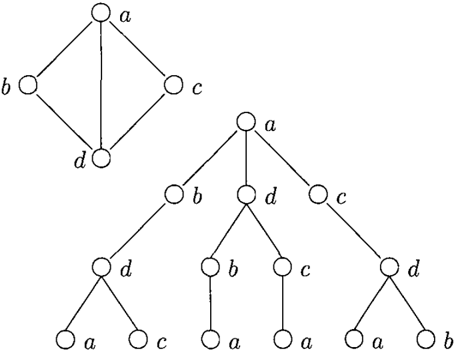
Definition 2.6 Given a pairwise potential <P and its graph (S<P, E<P), the associated computation tree of depth n with root s E s<�> ' denoted (S�··, E�··), is de­ fined as the tree that consists of all length n paths in the graph, (S<P,E<P), starting at io = s, (io, iJ, i2, ... , in), that never backtrack. Specifically the tree consists of all length n paths where { ik, ik+J} E E<P and ik ,P ik+2.

Figure one shows an example of a computation tree of depth three starting at node a. In the figure we have labeled each node in the computation tree with the associated node in the original graph.

We want to construct a Gibbs measure whose Markov graph is the computation tree. For each edge and non­ leaf node we will place a potential corresponding to the potential on the original graph. We need only de­ fine the set of boundary self-potentials on the leaves in terms of the initializing messages. For each (i, j) E 15<�> let

Note that in the case when the initial messages are all set to the ones vector we have <I>�'0 1 = 0.

Definition 2. 7 Given 1>, its associated computation tree, (S�·s, E�·8), and a set of boundary self-potentials { q,;-+ j } (i,j) EE"' define the associated potential for the computation tree of depth n, denoted <I> n ,s, as follows:

1. Let the map r n : S�·· --+ sip be the map that takes node I to its associated node i in the original graph. (As constructed in definition 2. 6.)

1. For each I E S�·· let

Let J.LiP" · ' (w) be the measured determined by <I> n ,s. By construction, running LBP ( in this case BP ) to com­ pute the belief at the root node, s, of the computation tree of depth n is equivalent to computing the belief at node s on the original graph after n iterations of LBP initialized appropriately.

3 Convergence of LBP and the Weak Limit

A sequence of measures {J.LiP"·' }n>I has a weak limit if for each N there exists a measur ; J.LN defined on s�·· such that for all events A E Fs"'· ' we have N

Proposition 3.1 The LBP algorithm converges if and only if the sequence of measures { J.LiP" · ' }n2:I has a weak limit.

Proof: We sketch the proof. Full details can be found in [3]. Using proposition 2.1 and the definition of the computation tree we have\;/ n > Nand\;/ ( E fls"'· ' : N

For fixed N the boundary I8S�··1 is finite. If LBP converges then the second factor above converges, as n--+ oo, to fl;EaS�·· m(AN (i), AN (i s "' ·')) (( ) and hence N the weak limit exists. A similar argument proves the other direction. D

Our goal for the rest of the paper is to understand the convergence properties of the sequence of measures

{J.LiP"·' }n>I · However, instead of working with a se­ quence of finite trees of increasing depth we will find it easier to study one infinite tree and the measures defined on it.

4 Gibbs Measures Over a Countable Set of Sites

Constructing a Gibbs measure over a countable set of nodes can be a tricky business. For example, there can be many Gibbs measures consistent with a given local specification provided by the potentials. This section is devoted to the construction of these Gibbs measures.

4.1 Specifications

We now let the set of nodes S be countably infinite and redefine

to be the set of all nonempty, finite, subsets of S. At every node i E S there is a finite measure space ( X;, F;). We construct, in the usual way, the product measure space (!1, F) = (fli ES X;, fliES F;). We also extend the uniform reference measure >. = fli ES >.; on (!1, F). As before we restrict ourselves to pairwise po­ tentials. We assume that the number of neighbors at any node is finite and hence for any A E § the energy Hf(w) = LAE§, AnA,<0 1>A(w) exists.

Because there are a countably infinite number of nodes we cannot compute the partition function by summing over all nodes. But we can discuss the partition func­ tion when conditioned on a particular boundary. De­ fine the partition function in A E § for the potential 1>, boundary w S\ A , and reference measure >. to be

Definition 4.1 Given a potential <I>, w E !1, and A E §. Then the measure

is called the Gibbs distribution in A with boundary WS\A and potential 1>. Furthermore "(if> = b A } A E S is called the Gibbsian specification for 1>.

Given a Gibbsian specification, which is a local de­ scription of a measure, we can ask how many mea­ sures are consistent with it. Define the set of Gibbs measures for the potential 1> to be

The following proposition gives us an implicit charac­ terization of the elements in G('Y<t>).

Proposition 4.1 fl. E G('Y<t>) if and only if WYl = fl., VA E §

Proof: See [1].0

The equations wrl = fl., VA E § are called the DLR equations after Dobrushin, Langford, and R uelle. They state that

This is a restatement of the fact that the iterated con­ ditional expectation equals the unconditional expec­ tation. The DLR equations will play a very impor­ tant role in our subsequent analysis. One can think of G("Y<t>) as the set of all measures locally consistent with the specified potential <I>. Said another way G("Y<t>) is the set of all measures preserved under a countable number of proper probability kernels: bl(I w)}AES·

For the pairwise potential, <P, one can show that each fl. E G('y<t>) is a Markov field. Specifically

This is sometimes called the local Markov property. We will discuss the global Markov property when we discuss Markov chains on trees in the next subsection.

Characterization of G(/'4>)

The set G("Y<t>) can either be empty, contain one mea­ sure, or contain an infinite number of measures. A potential is said to exhibit a phase transition if the set IG("Y<f>)l > 1. P hase transitions are a remarkable phe­ nomena. For a given local specification we can have very different global behaviors. For a proof of the fol­ lowing proposition see [1].

Proposition 4.2 Let <I> be an admissible, pairwise po­ tential defined on the countably infinite set of nodes S. There exists at least one Gibbs measure for an admis­ sible pairwise potential <P.

We have just shown that G("Y<t>) is nonempty. We now discuss its structure. Clearly it is a convex set because the convex combination of two elements in G(/4>) will certainly be a member of G(l<t>). To prove this it is enough to show that the convex combination satisfies the DLR equations.

Furthermore we can characterize the extreme points of the convex set G('y<t>). R ecall an element of a con­ vex set is extreme if it cannot be represented as the convex combination of other elements in the set. Each extremal element of G(/4>) is called a phase. Define the tail sigma field to be T � nAE§:FA'.

Proposition 4.3 Let fl. E G(/4>) then the following are equivalent

1. fl. is extreme
2. fl. is trivial on the tail sigma field T
3. for all cylinder events A

Proof: See propositions 7.7 and 7.9 of [1]. 0

An extremal measure is a mixing measure in the sense of point (3). If there is a unique measure G(l<f>) ={fl.} then that 11 is necessarily extremal, tail-trivial, and mixing.

4.2 Markov Fields on Trees: Boundary Laws, Markov Chains, and Limits

We have discussed Gibbs measures defined on count­ able sets of nodes. We now restrict our attention to Gibbs measures defined on infinite trees. We will show that if LBP converges then the associated measures on the computation tree must converge to an element of G(!<t>).

Limiting Gibbs Measures on Trees

How do we construct an infinite volume Gibbs mea­ sure? So far we only have an implicit characterization via the DLR equations. For Gibbs measures defined on infinite trees we will show that the measures can arise as the weak limit of a sequence of Gibbs measures with fixed boundary conditions.

Let <I> be a pairwise potential whose Markov graph (S<t>, E<t>) is a countably infinite tree. Let Tn c S<t> be the set of nodes in the tree that are a distance of n or less from the root. R ecall Ln C T n is the set of nodes that are exactly a distance n away from the root.

From the original potential <P = { <P A} we will now define a new sequence of potentials. For each n 2:: 1 define q, T n = { <P � n } by

where q, bd , n � { <P � ' n } represents added self-potentials at the leaves of the Tn tree. If <P � , n = 0 for all A C Ln then we call the boundary a free boundary. Note that "Yf n (A I w) is independent of w for A E :Fr n . For each q,Tn we can write the unique Gibbs measure as 4oTn o:f.!Tn fl. = AT�"'f T n '

In the context of the computation tree J.L .p r n rep­ resents the measure on the infinite tree correspond­ ing to n iterations of LBP when initialized with the self-potentials cpbd,n . We can relate the choice of cpbd,n to the choice of boundary self-potentials, { <I>!:->·; } ( . · )EE-, in the LBP algorithm. s.,s 1

We are interested in conditions that insure the mea­ sures, { J.L<P r " }n2:l, converge to a limiting measure. The next proposition states that if they converge to a lim­ iting measure then that measure must be an element of G ('Y <�> ) . Hence examining the structure of G('Y<P) is useful for determining convergence of LBP.

Proposition 4.4 Each subsequential limit of the se­ quence of measures { �t <P r " }n2:l belongs to G('Y<P).

Proof: We sketch the proof. For full details see [3]. Note that for each A E § there is an n large enough such that 1f" (- I w) = 1lC I w).

We need to show that the subsequential limits of the sequence of measures {J.L .p r n } n > l belong to G (<I>) . Let -T J.L be a subsequential limit where limk->oo J.L <P " · = It· We will show that J.L satisfies the DLR equations. Let A E § and let A be a cylinder event. Then IJ.L 'Yl (A) - J.L(A) I

where the second equality holds for k large enough so thatA CT n ,· 0

Markov Chains and Boundary Laws

We have just shown that each subsequential limit of the sequence of measures {�t .pT n }n2:l belongs to G('Y<�>). Here we describe the structure of the subsequential limits in terms of the Markov chains defined in G('y<P).

We are given a potential <I> with a countably infinite tree Markov graph ( s<�>, E<�>). Let

be the set of nodes in the "past" of the directed edge (i, j) including the node i.

Definition 4.2 A measure J.L<P is a Markov chain on the tree if

for all (i, j) E e<�> and Wj E

One can show that every Markov chain on the tree is a Markov field on the tree. The converse though does not always hold (see [ 1 ]. ) Measures that are Markov fields are often called two-sided whereas measures that are Markov chains are often called one-sided.

Proposition 4.5 Let <I> be a pairwise potential whose Markov graph is a tree. If It is an extremal element of G("y<l>) then it is a Markov chain.

Proof: See theorem 12.6 in [ 1]. 0

There can exist Markov chains that are not extremal. Thus extremality alone is not enough to characterize the Markov chains in G('y<�>). It turns out, though, that we can characterize each Markov chain by the use of boundary laws. We will then show that these boundary laws are related to the messages in LBP.

First define for each { i, j} E E<P a transfer matrix

We can then write

where here ZA(w) = l: wA TI{i,j}nA,<0 Q{i,j)(wi, W j) ·

Definition 4.3 A family { l (i, j)} (i, j)E E�, where each l ( i, J ) is a measure on Xi is called a boundary law if for each (i,j) E e<�> we have Vwi E Xi:

Note the similarity to the message passing update rule.

Proposition 4.6 The following hold

• (a) Each boundary law { l(i, j)} (i, j)EE� for the trans­ fer matrices { Q {i,j ) } {i, j}E E� defines a unique Markov chain It E G('y<P) vza the equation: for each connected set A

• (b) Each Markov chain It E G('y<P) admits a repre­ sentation of the form {3) in terms of a boundary law { l(i, j)} (i,j)EE� which is unique up to a positive scaling constant.

Proof: See theorem 12.12 of [ 1]. 0

1:1

80

Boundary Laws and Messages

Let .P be a pairwise potential whose Markov graph is an infinite tree. We now relate boundary laws to messages. R ecall that for each (i, j) E §<�> we have

Note that equation (2) has a product of sums form whereas the equation above has a sum of products from. For each (i,j) E fj<�> let

In summary, we have characterized each subsequential limit measure corresponding to the LBP algorithm in terms of a Markov chain defined on the computation tree. We will now discuss conditions that insure the existence of a unique limit.

5 Unique Gibbs Measure Case

Here we consider the case of a unique Gibbs mea­ sure: I G('Y<P) I = 1. Clearly there can be only be one subsequential limit of the sequence of measures J. I<P T" . Hence LBP converges. We can say something stronger though: LBP converges uniformly over the choice of all initializing messages.

and after some algebra we get

Proposition 5.1 If I G(!<I>)I = 1 then

which is in a product of sums form. Comparing (4) and (2) we see that

Thus we can go from boundary self-potentials and mes­ sages to boundary laws and vice-versa.

Proposition 4. 7 Each subsequential limit of the se­ quence of measures {J.t <PT" · h21 corresponds to a Markov chain in G('Y<�>).

Proof: We sketch the proof. See [3] for full details. Let {nk}k21 be a subsequence for which { J.t <PT " · h21 converges to some measure J.l · By proposition 4.4 this J.l is an element of G('Yot>). By proposition 3.1 the mes­ sages { m n( · . ) } converge along the subsequence { n k} t,] to some fixed point solution { m( i,j) }. By equation (2) and ( 4) this fixed point solution corresponds to a boundary law. By proposition 4. 6 we see that J.l is a Markov chain. 0

R ecall that proposition 4.2 states that the set G('y<P) is nonempty and hence contains at least one extremal element. By proposition 4. 5 this extremal element is a Markov chain. These results along with propositions 3.1 and 4.7 give us a new way to show that there al­ ways exists at least one solution to the LBP fixed point equations.

It has been observed in practice that LBP sometimes oscillates. In this case LBP is actually jumping be­ tween different solutions of the LBP fixed point equa­ tions and hence jumping between different Markov chains defined on the computation tree.

Proof: See proposition 7.11 in [I]. 0

Proposition 5.2 If I G(!<I>)I = 1 then for any cylinder event A we have

uniformly over the boundary self-potentials.

Proof: We sketch the proof. See [3] for full details. Let { .pbd, n } n > l be any set of boundary self-potentials. Let A be FA,-measurable and choose E > 0. Then by proposition 5.1 there exists a A2 :::l A1 such that I 'Y l,( A I w)- J.t<I>( A ) I ::; E. Now for T n :::l A2 we have

where the first equality holds via the DLR equa­ tion. Thus the convergence rate is independent of the boundary self-potentials used. 0

In summary if IG(.P)I = 1 then LBP will converge uniformly over the boundary self-potentials. Next we present Dobrushin's sufficient condition for uniqueness of the limiting Gibbs measure.

Dobrushin's Condition

A Gibbs potential can lead to many different phases if nodes that are far apart from each other do not mix fast enough. Dobrushin proposed the following condi­ tion that insures fast mixing and hence uniqueness.

Proposition 5.3 Let iP be a pairwise potential. If

then I G(r<l>)l = 1. Where 6(!) � supx f(x) -infx f(x).

Proof: See proposition 8.8 in [1]. 0

This proposition states that the " influence" node i has on the rest of the nodes depends on two things: the number of neighbors it has and the strength of the po­ tentials, measured by 6(<I>) , it takes part in. Note that the self-potentials do not play a part in Dobrushin's condition.

Let us return to the issue of LBP. Let iP be the poten­ tial for the finite Gibbs measure that we wish to apply LBP to. Let 1> be the corresponding potential on the computation tree. The local topology of the compu­ tation tree looks like the local topology of the original graph. Hence to show I G(<i>)l = 1 we need to show

Note that the maximum condition is very easy to check on finite graphs.

Rate of Convergence

Here we give a condition on the rate of convergence of LBP. Let c( <P) = m a.x s E S � l:A3s e2(IAI-1)6(<I>A)·

Proposition 5.4 If c( iP) < 2 then

where s is the root node and k = (1c(.P)) -1 zs a constant.

Proof: See theorem 8.23, remark 8.26, and corollary 8.32 of [ 1]. o

6 Conclusions

In this paper we have introduced tools from the theory of Gibbs measures to analyze the convergence proper­ ties of the LBP algorithm. In particular we related the problem of convergence of LBP to the existence of a weak limit for a sequence of Gibbs measures de­ fined the corresponding computation tree. We have introduced a condition that insures the uniqueness of the Gibbs measure defined on the infinite computation tree. Hence this condition insures LBP converges.

Acknowledgments

The authors would like to thank San joy Mitter, Kevin Murphy, and Mark Paskin for many helpful discussion.

This work was supported by the DoD Multidisci­ plinary University Research Initiative (MURI) pro­ gram administered by the Office of Naval Research under Grant N00014-00-1-0637.

References

1. H. 0. Georgii, Gibbs Measures and Phase Transi­ tions. Berlin, Walter de Gruyter and Co., 1988.
2. [ 2] F. Jensen, An Introduction to Bayesian Networks. UCL Press, London, 1996.
3. [ 3] S. Tatikonda and M. Jordan, " Conditions for Convergence in the Loopy Belief Propagation Al­ gorithm. " Berkeley working paper, 2002.
4. M. Wainwright, T. Jaakkola and A. Willsky, "Tree-Based Reparameterization for Approxi­ mate Estimation on Loopy graphs." Advances in Neural Information Processing Systems 14, 2002.
5. Y. Weiss, " Correctness of Local Probability Prop­ agation in Graphical Models with Loops." Neural Computation, 12:1-41, 2000.
6. J. Yedidia, W. Freeman. Y. Weiss, "Bethe Free Energy, Kikuchi Approximations and Belief Prop­ agation Algorithms." Advances in Neural Infor­ mation Processing Systems 13, 2000.
7. A. Yuille, "A Double-Loop Algorithm to Mini­ mize the Bethe and Kikuchi Free Energies." Neu­ ral Computation, to appear, 2001.