Contents
1301.0592
MAP Complexity Results and Approximation Methods
Jaiiles D. Park Computer Science Department University of California Los Angeles, CA 90095 jd@cs. ucla.edu
Abstract
MAP is the problem of finding a most prob able instantiation of a set of variables in a Bayesian network, given some evidence. MAP appears to be a significantly harder problem than the related problems of com puting the probability of evidence (Pr), or MPE (a special case of MAP). Because of the complexity of MAP, and the lack of viable al gorithms to approximate it, MAP computa tions are generally avoided by practitioners.
This paper investigates the complexity of MAP. We show that MAP is complete for NP PP . We also provide negative complex ity results for elimination based algorithms. It turns out that MAP remains hard even when MPE, and Pr are easy. We show that MAP is NP-complete when the networks are restricted to polytrees, and even then can not be effectively approximated.
Because there is no approximation algo rithm with guaranteed results, we investigate best effort approximations. We introduce a generic MAP approximation framework. As one instantiation of it, we implement local search coupled with belief propagation (BP) to approximate MAP. We show how to ex tract approximate evidence retraction infor mation from belief propagation which allows us to perform efficient local search. This al lows MAP approximation even on networks that are too complex to even exactly solve the easier problems of computing Pr or MPE. Experimental results indicate that using BP and local search provides accurate MAP es timates in many cases.
1 Introduction
The task of computing the Maximum a Posteriori hy pothesis (MAP) is to find the most likely configuration of a set of variables (which we will call the MAP vari ables) given (partial) evidence about the complement of that set (the non-MAP variables).
One specialization of MAP which has received a lot of attention is the Most Probable Explanation (MPE). tiation for the complement of that set. The primary that MPE seems to be a
MPE is the problem of finding the most likely config uration of a set of variables given an evidence instan reason for this attention is much simpler problem than its MAP generalization.
Unfortunately, MPE is not always suitable for the task of providing explanations. For example, in system di agnosis, where the health of each component is rep resented as a variable, one is interested in finding the most likely configuration of health variables only - the likely input and output values of each component are not of interest. Additionally, the projection of an MPE solution on these health variables is usually not a most likely configuration. Nor is the configuration obtained by choosing the most likely state of each variable sep arately.
MAP turns out to be a very difficult problem even when compared to MPE or computing the probabil ity of evidence (Pr). In section 2 we present some complexity results for MAP that indicate that neither exact nor approximate solutions can be guaranteed, even under very restricted circumstances. Still, MAP remains an important problem, and one we would like to be able to generate solutions for. Our approach is to provide best effort approximation methods. In sec tion 3 we discuss a general approach to approximating MAP and provide one instantiation of that approach that is based on belief propagation and local search, which allows MAP approximations even when exact MPE and Pr computations are not feasible.
-;
2 MAP Complexity
In this section, we begin by reviewing some complex ity theory classes and terminology that pertain to the complexity of MAP. Next, we examine the complex ity of MAP in the general case. We then examine the complexity of current state of the art MAP algorithms based on variable elimination. We conclude the com plexity section by examining the complexity of MAP on polytrees.
2.1 Complexity Review
We assume that the reader is familiar with the ba sic notions of complexity theory like the hardness and completeness of languages, as well as the complexity class NP. For an in-depth introduction to complexity theory see [13].
In addition to NP, we will also be interested in the class PP and a derivative of it. Informally, PP is the class which contains the languages for which there exists a nondeterministic Turing machine where the majority of the nondeteriministic computations accept if and only if the string is in the language. PP can be thought of as the decision version of the functional class #P. As such, PP is a powerful language. In fact NP C PP, and the inequality is strict unless the polynomi ;;i hierarchy collapses to the second level. 1
Another idea we will need is the concept of an oracle. Sometimes it is useful to ask questions about what could be done if an operation were free. In complexity theory this is modeled as a Turing machine with an oracle. An oracle Turing machine is a Turing machine with the additional capability of being able to obtain answers to certain queries in a single time step. For example, we may want to designate the class of lan guages that could be recognized in nondeterminstic polynomial time if any PP query could be answered for free. The class of languages would be NP with a PP oracle, which is denoted NP PP .
In this paper, we will be dealing with the decision versions of the problems. For example, the decision problem for MAP is: Given a Bayesian Network with rational parameters, a subset of its variables X, ev idence e (which consists of a partial instantiation of the non-MAP variables) and a rational threshold k, is there an instantiation x of X such that Pr( x , e ) > k? The decision problems for MPE and Pr are defined similarly.
'This is a direct result of Toda's theorem [20]. From Toda's theorem pPP contains the entire � olynomial hier archy (PH), so if NP = PP, then PH!;; p P = pNP _
2.2 MAP Complexity for the General Case
Computing MPE, Pr, and MAP are all NP-Hard, but there still appears to be significant differences in their complexity. MPE is basically a combinatorial opti mization problem. Computing the probability of a complete instantiation is trivial, so the only real dif ficulty is determining which instantiation to choose. MPE is NP-complete.2 Pr is a completely different type of problem, characterized by counting instead of optimization and is PP-complete [7] (notice that this is the complexity of the decision version, not the func tional version which is #P-complete [17]). MAP com bines both the counting and optimization paradigms. In order to compute the probability of a particular instantiation, an inference query is needed. Optimiza tion is also required, in order to be able to decide be tween the many possible instantiations. This is re flected in the complexity of MAP.
Proof: Membership in NP PP is immediate. Given any instantiation x of the MAP variables, we can verify if it is a solution by querying the PP oracle if Pr( x , e) > k.
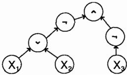
To show hardness, we reduce E-MAJSAT [10] (the canonical SAT oriented complete problem for NP PP ) to MAP. E-MAJSAT is defined as follows: Given a Boolean formula ¢ over n variables x 1 , ··· , Xn, and an integer k, 1 � k � n, is there an assignment to the first k variables such that the majority of the assignments to the remaining n - k variables satisfy ¢? First, we create a Bayesian Network that models the Boolean expression. For each variable in the expression, we cre ate an analogous variable in the network with uniform prior probability. Then, for each logical operator, we create a variable whose parents are the variables corre sponding to its operands, and whose CPT encodes the truth table for that operator (see Figure 1 for a simple example). Let V¢ be the network variable correspond ing to the top level operand. For a particular instan tiation x of variables X!,····Xk, we let e = {v¢ = T}. Then,
2 The NP-hardness of the functional version of MPE was shown in (19]. We are not aware of any published proof of the completeness of the decision problem, so we sketch it here. Membership is immediate, since the score for a purported solution can be tested in linear time. Hardness is based on using the standard Bayesian network simula tion of a Boolean expression (c. f. Theorem 1) to solve SAT. MPE(v¢ = T) > 0 if and only if the expression is satisfiable.
3This result was stated without proof in [9]. The author attributed the result [8] to an unpublished proof by Mark Peot.
= (#satisfied)/ 2°
Since there are 2 n - k possible instantiations of X k +t, ··· ,X n , we have
So the MAP query over variables Xt, ... , X k with evi dence vq, = T and threshold 1/2 k + 1 is true if and only if the E-MAJSAT query is also true. 0
This class has also been shown to be important in probabilistic planning problems [10].
NP PP is a powerful class, even compared to NP and PP. They are related by N P � PP � Np PP , where the equalities are considered very unlikely. In fact, NPPP contains the entire polynomial hierarchy [20].
Additionally, because MAP generalized Pr, MAP in herits the wild nonapproximability of Pr shown in [17].
Corollar l 2 For any E > 0, approximating MAP within 2" -· is NP -hard where n is the number of vari ables in the network.
So, if P i' NP then no polynomial time algorithm ex ists for approximating MAP that can guarantee subex ponential relative error.
2.3 Results for Elimination Algorithms
Solution to the general MAP problem seems out of reach, but what about for "easier" networks? State of the art exact inference algorithms (variable elimi nation [4], join trees [6, 18, 5], recursive conditioning [2]) can compute Pr(e) and MPE in space and time complexity that is exponential only in the width of the elimination order used. This allows many networks to be solved using reasonable resources even though the general problems are very difficult. Similarly, state of the art MAP algorithms can solve MAP with time and space complexity that is exponential only in width of the elimination order. Unfortunately, for MAP, not all orders can be used. In practice the order is gener ally generated by restricting the elimination order to eliminate all of the MAP variables last. This tends to produce elimination orders with widths much larger than those available for Pr and MPE, often placing exact MAP solutions out of reach [15]. We now con sider the question of whether there are less stringent conditions for valid elimination orders, that may allow for orders with smaller widths.
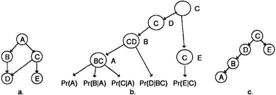
Elimination algorithms exploit the fact that summa tion commutes with summation, and maximization commutes with maximization in order to essentially factor the problem. Given an ordering, elimination al gorithms work by stepping through the ordering, col lecting the potentials mentioning the current variable, multiplying them, then replacing them with the po tential formed by summing out (or maximizing) the current variable from the product. This process can be thought to induce an evaluation tree. The evalu ation tree for an order consists of the potentials gen erated by performing the variable elimination, where an edge means that the child was one of the potentials that were combined to form the parent (see Figure 2 for an example). The width of the elimination order is the size (measured in the number of variables) of the largest potential in the evaluation tree.
Because maximization and summation do not com mute, not all variable orders generate evaluations that are valid. That is, trying to perform elimination us ing some orders will produce incorrect results. MAP requires that summation be performed before maxi mization. Thus, the criteria that needs to be satis fied is that a potential cannot be maximized if it men tions any summation variables. An elimination order is valid (because it generates a valid evaluation tree) if the induced evaluation tree never maximizes a variable out of a potential that mentions a summation variable. The standard way of ensuring a valid order is to elim inate all of the summation variables before any of the maximization variables. Two questions present them selves. First, are there valid orderings that interleave summation and maximization variables? And second, if so, can they produce widths smaller than those gen erated by eliminating all summation variables, then all maximization variables?
The answer to the first question is yes, there are other valid elimination orders. To see that, we introduce the notion of the elimination tree. An elimination or der induces an elimination tree which consists of the variables of the order, where an edge from parent to child indicates that the potential generated by elimi nating the child was combined to form the potential generated by eliminating the parent. The elimination tree can be thought of as a high level summary of the evaluation tree. Figure 2 shows a sample network and elimination order, with its associated evaluation
tree and elimination tree. The elimination tree de fines a partial ordering of the variables where a child in the tree must be eliminated before the parent. Any elimination order that obeys the partial order induces the same evaluation tree. Thus, if an order is valid, all other orders that share the same elimination tree are also valid. Additionally, since they share the same evaluation tree, they all have the same width. Figure 2 shows the tree induced by using the order AEBDC ( which eliminates summation variables first ) to solve MAP ( C,D ) . An equivalent order that interleaves sum mation and maximization variables is ABDEC. Typi cally, there are many valid interleaved elimination or ders. Unfortunately, allowing interleaved orders does not help.
Theorem 3 For any valid MAP elimination order, there is an ordering of the same width in which all of the maximization variables are eliminated last.
Proof: Consider the elimination tree induced by any valid elimination order. No summation variable is the parent of any maximization variable. This can be seen by considering any maximization variable. When the corresponding potential was maximized, it had no summation variables, and so the resulting potential also has no summation variables. Hence, any parent of a maximization variable must also be a maximization variable. Since no summation variable is a parent of a maximization variable, all summation variables can be eliminated first in any order consistent with the par tial order defined by the elimination tree. Then, all the maximization variables can be eliminated, again obeying the partial ordering defined by the elimina tion tree. Because the produced order has the same elimination tree as the original order, they have the same width. 0
2.4 MAP on Polytrees
Theorem 3 has significant complexity implications for elimination algorithms even on polytrees.
Theorem 4 Elimination algorithms require exponen tial resources to perform MAP, even on some polytrees.
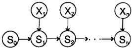
Proof: Consider computing MAP(X1 ... Xn, {Sn = T}) for a network consisting of variables Xb···,Xn,So, ... ,Sn with topology as shown in Fig ure 3. By Theorem 3, there is no order better than eliminating all of the non-MAP variables. But, after the non-MAP variables are eliminated, all of the MAP variables appear in a single potential. Thus the width is linear in the number of variables, and the algorithm requires exponential resources. 0
Which variables are maximized makes a crucial difference in the complexity of MAP computa tions. For example, the problem of maximizing over Xl···Xn/2,So ... Sn/2 instead of X 1 ... Xn can be solved in linear time.
It turns out that finding a good general algorithm for MAP on polytrees is unlikely.
Theorem 5 MAP is NP-Complete when restricted to polytrees.
Proof: Membership is immediate. Given a purported solution instantiation x, we can compute Pr ( x , e ) in linear time and test it against the bound. To show hardness, we reduce MAXSAT to MAP on a polytree. A similar reduction was used in [10] and [14]. The MAXSAT problem is defined as follows: Given a set of clauses C1, ... , Cm over variables X1, . .. , Xn and an integer bound k, is there an assignment of the vari ables, such that more than k clauses are satisfied. The idea behind the reduction is to model randomly se lecting a clause, then successively checking whether the instantiation of each variable satisfies the selected clause. The clause selector variable So with possible values 1, 2, ... , m has a uniform prior. Each proposi tional variable x; induces two network variables X; and S;. X; represents the value of x;, and has a uniform prior. S; represents whether any of x1, ··· , x; satisfy the selected clause. S; = 0 indicates that the selected clause was satisfied by one of x1, ··· ,x;. S; = c > 0
... -l
indicates that the selected clause Cc was not satisfied by XI. ... , x;. The parents of S; are x; and Si-1 (the topology is shown in Figure 3). The CPT for S;, for i 2:: 1 is defined as
In words, if the selected clause was not satisfied by the first i1 variables (S;_1 "I 0), and the x; satisfies it, then S; becomes satisfied (S; = 0) otherwise, S; = S;_1. Then for a particular instantiation c of So and x of X1, ... ,Xn, Pr(c, x, Sn = 0) = 1/(m2 n ) if x satisfies clause Cc, 0 otherwise. Thus MAP over X1, ... ,Xn with evidence Sn = 0 and bound k/(m2n) solves the MAX-SAT problem as well. D
Additionally, because MAX-SAT is MAXSNP complete, we have the following corollary:
Corollary 6 MAP on polytrees is MAXSNP -hard .
This means that there is no polynomial time approxi mation scheme for MAP on polytrees unless P = NP.
3 Approximating MAP
The complexity of MAP places exact solution out of reach in all but the simplest cases. Good approxi mations can not be guaranteed either. Still, we want some method to generate at least approximate solu tions to the problem. Typically practitioners resort to computing individual posteriors, or computing MPE, and projecting the solution onto the MAP variables. Unfortunately both methods in general produce rel atively poor approximations to MAP. Also, when the network is complex, both methods are too complicated to compute exactly.
We propose a general framework for approximating MAP. MAP consists of two problems that are hard in general - optimization and inference. A MAP ap proximation algorithm can be produced by substitut ing approximate versions of either the optimization or inference component (or both). The optimization problem is defined over the MAP variables, and the score for each solution candidate instantiation s of the MAP variables is the (possibly approximate) probabil ity Pr ( s , e ) produced by the inference method. This allows solutions tailored to the specific problem. For networks whose treewidth is manageable, but contains a hard optimization component (e.g. the polytree ex amples discussed previously), exact structural infer ence can be used, coupled with an approximate opti mization algorithm. Alternatively, if the optimization problem is easy (e.g. there are few MAP variables) but the network isn't amenable to exact inference, an exact optimization method could be coupled with an approximate inference routine. If both components are hard, both the optimization and inference components need to be approximated.
The only previous algorithlnB for approximating MAP of which we are aware are instantiations of this frame work. They both use an exact probability engine, but an approximate optimization engine [ 3 , 15], and so are feasible for networks amenable to exact inference.
We now present a new MAP approximation algorithm which uses local search to approximate the optimiza tion component, and belief propagation to approxi mate the inference component. This extends the realm of problems where MAP approximations can be effec tively generated to problems that can be approximated well by belief propagation.
Belief propagation has a number of qualities that make it a good candidate to use as the approximate prob ability engine for MAP approximation. Experimental results have shown impressive performance in a va riety of domains. It has effective methods for com puting MPE and posteriors of individual nodes, which are both powerful initialization methods for the local search. Recent work [21] has demonstrated how to use BP to estimate Pr(e), which is the primary re quirement for using it as a subroutine to MAP. Also, approximate retracted marginals Pr( x l e - X) can be computed locally for each variable. The notation e-X represents the instantiation formed by removing the assignment of X from e. The ability to approximate retracted marginals provides a linear speed up for the search.
3.1 Belief Propagation Review
Belief propagation was introduced as an exact infer ence method on polytrees [16]. It is a message passing algorithm in which each node in the network sends a message to its neighbors. These messages, along with the CPTs and the evidence can be used to compute posterior marginals for all of the variables. In net-
works with loops, belief propagation is no longer guar anteed to be exact and successive iterations generally produce different results, so belief propagation is typ ically run until the message values converge. This has been shown to provide very good approximations for a variety of networks [11, 12], and has recently received a theoretical explanation [22].
Belief propagation works as follows. Each node X, has an evidence indicator Ax where evidence can be entered. If the evidence sets X = x, then Ax (x) = 1, and is 0 otherwise. If no evidence is set for X, then Ax(x) = 1 for all x. After evidence is entered, each node X sends a message to each of its neighbors. The message a node X with parents U sends to child Y is computed as
where Z ranges over the neighbors of X and a is a normalizing constant. 4 Similarly, the message X sends to a parent U is
Message passing continues until the message values converge. The posterior of X is then approximated as
4 We use potential notation more common to join trees than the standard descriptions of belief propagation be cause we believe the many indices required in standard presentations mask the simplicity of the algorithm.
3.2 Description of the Algorithm
We use BP for the inference algorithm, and stochastic hill climbing as the optimization routine. The stochas tic hill climbing method performs local search in the space of MAP variable instantiations, looking for the optimal instantiation. It works by either greedily mov ing to the best neighbor, or stochastically selecting a neighbor, where the choice is made randomly with some fixed probability. In this algorithm, one instanti ation of the MAP variables is a neighbor of another if they differ only in the assignment of a single variable.
The score for a particular instantiation can be com puted using the method for approximating the proba bility of evidence given in [21]. Using this method to select the best neighbor to move to requires running belief propagation separately on each neighbor in or der to compute its score. We can do better than that by running belief propagation on the current state s, and using the messages to approximate the change in score that moving to a neighboring state x, sX would produce. The improvement from the current state s to the neighboring state x, s X is just the ratio of their probabilities
By dividing both numerator and denominator by Pr'(s-X, e), we get
where x. is the value that X takes on in s. So, given the ability to approximate retracted conditional proba bilities locally, we can compute the best neighbor after a single belief propagation.
Belief propagation is able to approximate retracted values for each variable efficiently based on the mes sages passed to that variable. For polytrees, the in coming messages are independent of the value of the local CPT or any evidence entered. Leaving the evi dence out of the product yields
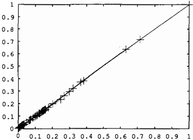
In multiply connected networks the incoming messages are not necessarily independent of the evidence or the local CPT, but as is done with other BP methods, we ignore that and hope that it is nearly independent. Empirically, the approximation seems to be quite accu rate. Figure 4 shows a representative example, com paring the correspondence between the approximate and exact retracted probabilities for 30 variables in the Barley network. The x axis corresponds to the
true retracted probability, and the y axis to the ap proximation produced using belief propagation.
Using retracted conditional probabilities to compute the improvement provides a linear speedup as com pared to using belief propagation to compute the score for each neighbor separately. Figure 5 provides pseu docode for the algorithm.
3.3 Initializing the Search
The performance of local search methods such as hill climbing often depend crucially on the initializa tion. We investigate two methods previously shown to be successful when using exact inference. The first method is based on MPE. It consists of computing the MPE assignment (which we approximate using the standard BP approximation method) then creat ing the MAP assignment by setting each MAP vari able to the value it takes on in the MPE assignment. The other method creates the instantiation by setting each MAP variable to the instance that maximizes Pr ' (XI e ), which we will call ML.
3.4 Experimental Results
We tested the algorithm on both synthetic and two real world networks from the Bayesian network repos itory [1]. For the first experiment, we generated 100 synthetic networks with 100 variables each using the method described in [15] with bias parameter 0.25 and width parameter of 13. We generated the net works to be small enough that we could often com pute the exact MAP value, but large enough to make the problem challenging. We chose the MAP variables as the roots (typically between 20 and 25 variables), and the evidence values were chosen randomly from 10 of the leaves. We computed the true MAP for the ones which memory constraints (512 MB of RAM) al lowed. We computed the true probability of the in stantiations produced by the two initialization meth ods. We also computed the true probability of the instantiations returned by pure hill climbing (i.e. only greedy steps were taken), and stochastic hill climbing (using p 1 = .3 and 100 iterations) for both initializa tion methods. Of the 100 networks, we were able to compute the exact MAP in 59 of them. Table 1 shows the number exactly solved for each method, as well as the worst instantiation produced, measured as the ra tio of the probabilities of the found instantiation to the true MAP instantiation. All of the hill climbing meth ods improved significantly over their initializations in general, although for 2 of the networks, the hill climb ing versions were slightly worse than the initial value (the worst was a ratio of .835), because of a slight mis match in the true vs. approximate probabilities. Over
| # solved exactly | worst | |
|---|---|---|
| MY.�<; | 9 | .015 |
| MPE-Hill | 41 | .06 |
| MPE-SHill | 43 | .21 |
| ML | 31 | .34 |
| ML-Hill | 38 | .46 |
| ML-SHill | 42 | .72 |
| min | median | mean | max | |
|---|---|---|---|---|
| MPE-Hill | 1.0 | 8.4 | 1.3xl0" | 3.1xl0"' |
| MPE-SHill | 1.0 | 8.4 | 1.3xl0 11 | 3.1x10 12 |
| ML-Hill | l.Ox10 4 | 3.6xl0 7 | 3.4x10 15 | 8.4xl0 16 |
| ML-SHill | 7.7x10 3 | 3.6x10 7 | 3.4xl0 15 | 8.4x10 16 |
all, the stochastic hill climbing routines outperformed the other methods.
In the second experiment, we generated 25 random MAP problems for the Barley network, each with 25 randomly chosen MAP variables, and 10 randomly chosen evidence assignments. We use the same pa rameters as in the previous experiment. The problems were to hard to compute the exact MAP, so we report only on the relative improvements over the initializa tion methods. Table 2 summarizes the results. Again, the stochastic hill climbing methods were able to sig nificantly improve the quality of the instantiations cre ated.
In the third experiment, we performed the same type of experiment on the Pigs network. None of the search methods were able to improve on ML initialization. We concluded that the problem was too easy. Pigs has over 400 variables, and it seemed that the evidence didn't force enough dependence among the variables. We ran another experiment with Pigs, this time using 200 MAP variables and 20 evidence values to make it more difficult. Table 3 summarizes the results. Again, the stochastic methods were able to improve significantly over the initialization methods.
Given: Bayesian network N, evidence e, and MAP variables S. Compute: An instantiation s which (approximately) maximizes Pr(s, e). Initialize current state s to some instantiation of S. Sbe.st = S Repeat many times: Perform belief propagation on N with evidence s, e. ifPr'(s,e) > Pr'(s&est,e) then Bbest = S With probability p 1 do Randomly modify one of the variable assignments in s. otherwise do Compute improvement(x,sX)= Pr'(xls- X,e)/Pr'(x.ls- X, e) for each neighbor x ,s -X. if improvement(x, s - X) < 1 for all neighbors Randomly modify one of the variable assignments in s. else Set s to the neighbor x, sX that has the highest improvement. return S&est| min | me<11an | mean | max | |
|---|---|---|---|---|
| MPE-Hill | 1.0 | 1.7x10" | 1.5x10' | 3.3x10• |
| MPE-SHill | 1.0 | 2.5x10⁵ | 4.5x10ll | 1.1x10 13 |
| ML-Hill | 13.0 | 2.0xl0 3 | 3.3x10⁵ | 4.5x10 6 |
| ML-SHill | 13.0 | 1.2x10 4 | 8.2x10⁵ | 8.2x10 6 |
4 Conclusion
MAP is a computationally very hard problem which is not in general amenable to exact solution even for very restricted classes (ex. polytrees). Even approxima tion is difficult. Still, we can produce approximations that are much better than those currently used by practitioners (MPE, ML) through using approximate optimization and inference methods. We showed one method based on belief propagation and stochastic hill climbing that produced significant improvements over those methods, extending the realm for which MAP can be approximated to networks that work well with belief propagation.
Acknowledgement
This work has been partially supported by MURI grant N00014-00-1-0617
References
- Bayesian network repository. www.cs.huji.ac.ilflabs/compbio/Repository.
- A. Darwiche. Recursive conditioning. Artificial Intell igence, 126(1-2):5-41, February, 2001.
- L. de Campos, J. Gamez, and S. Moral. Partial abductive inference in Bayesian belief networks using a genetic algorithm. Pattern Recognition Letters, 20(11-13):1211-1217, 1999.
- R. Dechter. Bucket elimination: A unifying framework for probabilistic inference. In 12th Conference on Uncertainty in Artificial Intell i gence, pages 211-219, 1996.
- F. V. Jensen, S. L. Lauritzen, and K. G. Olesen. Bayesian updating in recursive graphical models by local computation. Computational Statistics Quarterly, 4:269-282, 1990.
- S. L. Lauritzen and D. J. Spiegelhalter. Lo cal computations with probabilities on graphical structures and their application to expert sys tems. Journal of Royal Statist ics Society, Series B, 50(2):157-224, 1988.
- M. L. Litmman, S. M. Majercik, and T. Pitassi. Stochastic boolean satisfiability. J oumal of Au tomated Reasoning, 27(3):251-296, 2001.
- M. Littman. Personal comunication.
- M. Littman. Initial experiments in stochastic sat isfiability. In Sixteenth Nat ional Conference on Artificial Intelligence, pages 667-672, 1999.
- M. Littman, J. Goldsmith, and M. Mundhenk. The computational complexity of probabilistic planning. Journal of Artificial Intelligence Re search, 9:1-36, 1998.
- R. J. McEliece, E. Rodemich, and J. F. Cheng. The turbo decision algorithm. In 33rd Aller ton Conference on Communications, Control and Computing, pages 366-379, 1995.
- (12] K. P. Murphy, Y. Weiss, and M. I. Jordan. Loopy belief propagation for approximate inference: an emperical study. In Proceedings of Uncertainty in AI, 1999.
- C. Papadimitriou. Computational Complexity. Addison-Wesley, Reading, MA, 1994.
- C. Papadimitriou and J. Tsitsiklis. The complex ity of Markov decision processes. Mathematics of Operations Research, 12(3):441-450, 1987.
- J. D. Park and A. Darwiche. Approximating map using local search. In 17th Conference on Un certainty in Artificial Intelligence, pages 403-410, 2001.
- J. Pearl. Probabalistic Reasoning In Intelligent Systems. Morgan Kaufmann, 1998.
- D. Roth. On the hardness of approximate reason ing. Artificial Intelligence, 82(1-2):273-302, 1996.
- P. Shenoy and G. Shafer. Propagating belief functions with local computations. IEEE Expert, 1(3):43-52, 1986.
- (19] S. E. Shimony. Finding maps for belief networks is NP-hard. Artificial Intelligence, 68(2):399-410, 1994.
- (20] S. Toda. PP is as hard as the polynomial-time hierarchy. SIAM Journal of Computing, 20:865877, 1991.
- [21) Y. Weiss. Approximate inference using belief propagation. UAI tutorial, 2001.
- [22) J. Yedidia, W. Freeman, andY. Weiss. Gener alized belief propagation. In NIPS, volume 13, 2000.