Marginalizing in Undirected Graph and Hypergraph Models

Enrique F. Castillo

Dept. of Applied Mathematics and Computational Sciences. University of Cantabria 39005 Santander, Spain e-mail:castie@ccaix3. unican.es

Juan Ferrandiz

Department of Statistics and Operations Research, University of Valencia, Dr. Moliner 50, E-46100, SPAIN e-mail: [email protected]

Abstract

Given an undirected graph g or hypergraph 'H model for a given set of variables V , we introduce two marginalization operators for obtaining the undirected graph YA or hy­ pergraph 'HA associated with a given subset A c V such that the marginal distribution of A factorizes according to YA or 'HA, respec­ tively. Finally, we illustrate the method by its application to some practical examples. With them we show that hypergraph models allow defining a finer factorization or performing a more precise conditional independence anal­ ysis than undirected graph models.

1 INTRODUCTION

In many practical situations the structural relation­ ship among a set of variables V = { V1, . . . , Vn} can be represented as an undirected graph g = (V, E), where E is the set of edges of g. If two variables are indepen­ dent, the corresponding nodes should not be connected by a path.

Similarly, if the independence between variables X and Y is indirect and mediated by a third variable Z (that is, if X and Y are conditionally independent given Z), we display Z as a node that intersects the path between X and Y, i. e. , Z is a cutset separating X and Y. This correspondence between conditional in­ dependence and cutset separation in undirected graphs forms the basis of the theory of Markov fields (Isham [5], Lauritzen [6], Wermuth and Lauritzen [10]) , and has been given axiomatic characterizations (Pearl and Paz [11] ) .

However, in many practical cases we can be interested not in the whole set of variables V but in a subset A of them. In this case the initial graph model is not the most appropriate to work with and we are interested in the graph model induced by the initial graph in A.

The independence graph of marginal probability distri­ butions for a subset of the considered variables was un-

Pilar Sanmartin

Department of Mathematics, Jaume I University Castellon, SPAIN

e-mail: sanmarti@mat. uji.es

dertaken in Frydenberg (1990), after Asmussen (1983). There, he stated the collapsibility condition for the corresponding subgraph to be the independence graph of the marginal probability distribution.

Unfortunately, not all probabilistic models can be rep­ resented by undirected perfect maps. Pearl and Paz [11] characterize the dependency models represented by undirected perfect maps. The theorem refers not only to probabilistic but to general dependency mod­ els.

Since the resulting independence graph reveals this lack of sensitivity to detect all independence properties and lack identification of missing n-th ( n > 2) order in­ teractions when second order interactions are present, as an alternative, we use hypergraph models (see Rose [12], Tarjan and Yannakakis [13] , Mellouli [9] , Studeny [16] and Shafer and Shenoy [15] for related problems). In this paper, based on the factorization properties, we give an algorithm for obtaining the marginal indepen­ dence graph under general conditions. To illustrate these concepts, we use some examples in which this lack of sensitivity and the characteristic contribution of hypergraph models become apparent.

In Section 2 we introduce the main concepts to be used in the rest of the paper with a distinction between those required for the case of graphs and those for hy­ pergraphs. In particular, we introduce the hypergraph models based on Gibbs distributions. In Section 3 we introduce a marginalization operator for the case of undirected graphs that allows obtaining such a graph in the sense of the marginal model to satisfy the cor­ responding factorization properties. We also give an algorithm to implement this operator. In Section 4 we follow exactly the same process for the case of hyper­ graphs. In both sections we illustrate the methods by means of practical examples. Finally, we make some comparisons, and in Section 6 we give some conclu­ sions and recommendations.

2 BACKGROUND

We divide this section in two parts. The first is devoted to undirected graphs, and the second to Gibbs distri-

butions and hypergraphs. We assume that the range of every variable is a real set containing the zero.

2.1 UNDIRECTED GRAPHS

The main theorem to be given in Section 3 requires several concepts of undirected graphs which are given below. We illustrate them with some examples.

Definition 1 (Path). Given a graph g a path of length n between nodes Vr and V8 is a sequence of nodes Vo, ... , Vn such that (Vi, Vi+ I); i = 0, . . . , n -1 are edges of Q and Vo = Vr and Vn = Vs.

Definition 2 (Connected Nodes). Given a graph Q = ( V, E), two nodes Vr, V8 E V are said to be con­ nected if there is a path from Vr to Vs . They are said to be directly connected iff the path is of length 1.

Definition 3 (Complete Set). Given a graph g = ( V, E), a set A s:;;: V is said to be complete if all nodes in A are mutually and directly connected by edges in E.

Definition 4 (Clique). A maximal complete set of nodes is called a clique.

Definition 5 (Boundary). Given a graph g = ( V, E) and a subset A c V the boundary bd( A) of A is the set of nodes Vr tf. A such that they are directly connected to an element of A, i. e. ,

Definition 6 (Connectivity Components).

Given a graph g = ( V, E) its set of nodes V can be partitioned in maximal subsets of nodes which are mu­ tually connected (see Lauritzen {1996}, page 6}. These sets are called connectivity components of g.

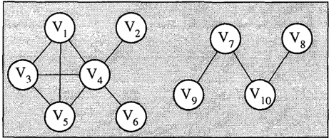
Example 1 Consider the set of variables V {V1, V2, ... , V10} and the graph Q = ( V, E) shown in Figure 1, where

Some illustrative examples of the above definitions are:

Path: The sequence of nodes {V1, V4, V5, V3} is a path of length 3 between vl and v3, as it is the sequence {V1, V3}, which has length 1.

Connected nodes: The nodes V8 and Vg are connected nodes because there is a path {Vs, Vw, V7, V g } joining VB and Vg.

Directly connected nodes: Nodes V7 and Vw are di­ rectly connected nodes because the path {V7, V1o} join­ ing them has length l.

Complete Sets: The only complete set of four elements in g is {V1, V3, V4, V 5 } (all pairs of nodes are directly connected). Obviously, all its subsets are also complete and it contains the only four complete sets of three elements. The remaining complete sets contain one or two elements.

Clique: The sets {V1, V3, V 4, V5}, {V4, V2}, {V4, V6}, {V7, V g }, {V7, Vw} , {Vs, Vw} are the cliques ofQ.

Boundary Set: The boundary of the set {V1, V3, V4, %} is the set {V2, V6}·

Connectivity components: The connectivity compo­ nents of the graph g are

Definition 7 (Completed Edge Set). Given a graph g = ( V, E) and a subset A c V, the completed edge sets E * ( A ) of A is the set of all possible edges between nodes in A.

Definition 8 (Subgraph). Given a graph g = ( V, E) and a subset A C V, the subgraph g A is the graph 9A = ( A, EIA) , that is, the graph defined over A and containing the edges of E connecting nodes in A.

Definition 9 (Factorization Property). A prob­ ability distribution P on V, is said to factorize ac­ cording to an undirected graph g (U DC), if for all complete set, C , of vertices there exist non-negative functions '1/Jc such that

The above factorization can be done using only cliques. However, this leads to a coarser factorization.

Example 2 Consider again the graph in Example 1.

Completed edge set: The completed edge set of the set {V7, Vs, Vg} is {(V7, Vs), ( V7, V g), ( V s, V g) } .

Subgraph: The subgraph associated with the set {V2, V4, V5, V6} is

Factorization: A possible factorization of p( v) is

2.2 GIBBS DISTRIBUTIONS AND HYPERGRAPHS

As it is well known undirected graphs do not lead to the finest possible factorization in probabilistic mod­ els. This justifies the use of the Gibbs and hypergraph models to be given below.

Definition 10 (Gibbs Model). Given a graph 9 = (V, E), the set of random variables V is said to follow a Gibbs model according to the graph 9 if its associated probability density function (pdf) can be written in the form

where K is a normalizing constant and C is the class of all complete sets of V with respect to 9. The func­ tions U c are called interaction functions and some of them can be null. {In order to avoid trivial undeter­ minations we will assume hereafter u(/J ( -) = 0).

Note that Expression (1) shows a characteristic factor­ ization property of the corresponding Gibbs model. In fact the density in ( 1) factorizes as

where the factors in {7/Jc(c)IC E C} are positive.

The above interpretation of the joint density in terms of the interaction functions is not unique. However, we are interested in the simplest possible representa­ tion, which is given by the normalized potential. In it an interaction function Uc(c) appears iff it cannot be written in terms of a sum of functions with less arguments.

Definition 11 (Normalized Potential). A poten­ tial U such that U c (c) = 0 whenever some component of c is null is called a normalized potential.

It can be shown that this potential is unique ( see Win­ kler (1995)) . In addition, any given potential U0 can be normalized in the sense of leading to the same joint distribution for V, by means of

This last equation makes evident that the normalized potential produces a finer factorization (2) of the pdf, because for every non-null interaction function Uc(c) of the normalized potential there is at least one non­ null interaction function Ujj (d) involving a bigger set of variables.

Definition 12 (Potential Restricted to a Set). Given a potential U on the set V and a subset A c V the potential UIA restricted to A is the set

Example 3 Consider the set of variables V {V1, V2, V3, V4, V s , V6} and the graph 9 = (V, E), where

Gibbs Model: Let us assume the following density:

with associated potential U0:

where eij are constants.

Normalized Potential: The corresponding normalized potential U becomes:

Potential Restricted to a Set: Given the set A = {V1, V3, V s }, the potential restricted to A is:

Definition 13 (Hypergraph). Given a set V, an hypergraph is a subset of parts of V.

Definition 14 (Hypergraph associated with a family of potentials. Hypergraph Models). Given a parametric family of potentials, the hypergraph associated with its normalized potential ue is de fined as the class of all sets of V with non-null interaction function ug for at least one element in the family, i. e.:

The corresponding model is called an interaction junc­ tions hypergraph or simply hypergraph model.

Note that hypergraph models are more capable to dis­ tinguish models than undirected graph models. For example, the last models cannot distinguish between the hypergraph model with potential (5) and the hy­ pergraph model with potential

(7)

Every hypergraph H on V induces in V the graph 9(1-i) = (V, E), where

The graph 9(1-i) associated with the hypergraph of a family of potentials verifies the factorization property with every probability distribution induced by these potentials.

Definition 15 (Hypergraph Partial Ordering). Given two hypergraphs 1i 1 and 1{2 on V, we say that 1i1 precedes H2 iff every element of 1i1 is contained in an element oj1i2, that is,

Comparing again the potentials in (5) and (7), we can say that the hypergraph associated with (5) precedes the hypergraph associated with (7) , but not conversely.

Now we can state the property of normalized poten­ tials producing finer factorizations in the more pre­ cise terms of partial ordering of the associated hyper­ graphs. The hypergraph associated with the normal­ ized potential precedes the hypergraph associated with any other potential leading to the same probability dis­ tribution.

Definition 16 (Boundary Hypergraph). Let H be the hypergraph and A C V. The boundary hyper­ graph HA of V \ A is the hypergraph of all subsets of A which are the boundary of some connectivity com­ ponent of 9v\ A in 9(1-l).

Example 4 Consider again Example 3.

Hypergraph associated with a family of potentials: The hypergraph associated with the potential U is

Graph associated with a hypergrapll.· The graph asso­ ciated with hypergraph H is

Boundary Hypergraph: Given A= {VI, V3, Vs}, since the connectivity components of V \ A are

the boundary hypergraph HA of V\A is the hypergraph:

3 THE MARGINAL OPERATOR FOR UNDIRECTED GRAPHS

Theorem 1 (The marginalization theorem for undirected graphs). Let g be the undirected graph (V, E), and P the probability distribution over V. If A c V and P A is the marginal distribution associated with A, we have that if P factorizes according to the graph g, then, the marginal distribution P A factorizes according to the graph gAa = (A, EAa), where

and T is the set of connectivity components of 9v\ A·

Proof: The marginal distribution is obtained by integration over de range of Z = V \ A, that is:

Replacing the value of p in terms of its factors and assuming that C varies in the class of all complete sets C, we get:

Thus, where

Let T be the set of connectivity components of the subgraph 9v\ A · Obviously, there are no elements inC with indices in more than one of these different compo­ nents. Thus, the integration over V\A in (9) factorizes in integrals, each on a connectivity component, as:

where each factor is of the form:

a function of the set of locations in A which are neigh­ bors of some location in the connectivity component r, that is, the set bd(r). Then, Co= UrET bd(7).

We shall write (9) as:

Consequently, the marginal pdf can be written as:

where we can see that the distribution P A satisfies the factorization property with respect to gAa = (A, EAa), as was to be proven. ·

This operator reminds us, in a certain way, the moral­ ization of chain graphs, the difference being that this applies to chain graphs (with the existence of arrows) to obtain a directed graph, by "marrying" the parents of each chain component. This new operator applies to undirected graphs and what get married are the elements in the boundaries of the connectivity compo­ nents of the locations associated with variables disap­ pearing during the marginalization process.

The above theorem suggests the following algorithm for marginalization.

Algorithm 1 Marginalization

Input: A graph Q = (V, E) and a subset A C V.

Output: A graph 9:4w = (A, E1,;:a) such that the A­ marginal of the graphical model associated with the graph Q factorizes according to 9:4w.

Step 1: Obtain the set E IA ( edges in QA)·

Step 2: Obtain the subgraph 9v\A.

Step 3: Obtain connectivity components T of QV\A·

Step 4: Determine the set bd( r) in Q for each r E T.

Step 5: Obtain the completed edge sets E*(bd(r)) for each rET.

Example 5 Assume the graph Q = (V, E), where

If we apply the Algorithm 1, we obtain:

Step 1: E IA = 0.

Assume that now we add the edge (VI, V3) to E. If we apply the Algorithm 1, we obtain:

Note that in both cases we obtain the same marginal graph.

4 THE MARGINAL OPERATOR FOR HYPERGRAPHS

In this section we analyze the marginalization problem in hypergraphs models.

To this aim we use the following theorem, where we state the potential U A corresponding to the family of marginal distributions P! in terms of the changes suf­ fered by the original potential U restricted to the set A. From the proof of theorem 1 we have seen the role of the connectivity components r of the subgraph 9v\A. In fact, we could call their contributions to the marginal potential U A the innovations of the poten­ tial U. They can be computed for each B <;;;;A as the double sum

if there is D in 'H A including B, (B =f. 0), and 0 oth­ erwise, where

with

Now, we shall state without proof the following the­ orem ( Sanmartin (1997)) for the parametric potential ue of a hypergraph model, where we add the e super­ script to all the functions derived from ue whenever we want to emphasize their parametric character.

Theorem 2 (The marginalization theorem for interaction hypergraphs). Consider a parametric family of Gibbs models over V, with interaction func­ tions hypergraph 'H, and P! be the corresponding fam­ ily of marginal distributions over A. Then, the inter­ action function hypergraph 'HA of the family P! can be expressed as:

where

1. 'HI A is the restriction of 'H to A, that is, the set of elements in 'H which are subsets of A.
2. H1 is the family of subsets B <;;;; A not in 'HIA and such that 8Vf(b) is a non-null function for some e. (These are the new complete sets that will appear after marginalization).
3. 'H"A is the set of complete sets in 'HIA such that they are subsets of some set in 'H A and satisfy the equation:

(These are the complete sets that will disappear after marginalization).

The decomposition of 'HA above, exhibits the neces­ sary and sufficient conditions for graphical and para­ metric collapsibility. It becomes apparent from (16) that the graph Q('HA) associated with the marginal

hypergraph coincides with the subgraph Q(H)A Q(HI A ) iff H� � HI A and (HA. = 0 or HA. -< (HIA \ HA.)). 三

If, in addition, we require parametric collapsibility (UIA = U A ), that is, the marginalizing operation not to change the interaction functions involving variables in A, the necessary and sufficient condition becomes that all innovations Vf(b) in (13) be null.

This theorem suggests the algorithm below for marginalizing a hypergraph. In it we clarify the mean­ ing of the sets and functions appearing in Expressions (13) and (15), which are not easy to understand. With the same purpose we also include a simple example.

Algorithm 2 Marginalization of Hypergraphs.

• Input: A set V, a parametric family of normal­ ized potentials U8 over V, and a subset A c V.
• Output: The A-marginal potential 8U A , to­ gether with its associated hypergraph HA and graph Q(HA)·

Step 1: Obtain the hypergraph H associated with the given potential U.

Step 2: Obtain the graph Q(H) associated with the hypergraph.

Step 3: Determine the connectivity components of the subgraph associated with V \ A.

Step 4: Obtain the boundary hypergraph H A , as the collection of the boundaries in Q(H) of the connectivity components of V \ A.

Step 5: For each element BE H A and each T verifying bd(r) =Bin (15) calculate the functions U J3 (b) .

Step 6: For each element BE H A calculate the func­ tions U'B(b) (see (14)) .

Step 7: Using (13), calculate Vf(b) for each non-void subset B of the sets in HA .

Step 8: Calculate the A-marginal potencial UA by adding V A to the initial potential U restricted to A.

Step 9: Obtain the hypergraph HA associated with u A .

Step 10: Obtain the graph Q(HA) associated with u A .

Example 6 Assume the set

of binary (0, 1) variables, the normalized potential

and the V -subset A= {V1, V3, V5}.

Step 1: The hypergraph H associated with the given potential U is

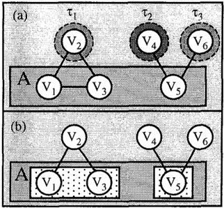
Step 2: The graph associated with the hypergraph is given in Figure 2( a)

Step 3: The connectivity components of the subgraph associated with V \ A are

as it can be seen in Figure 2( a).

Step 4: Since the boundaries of the connectivity com­ ponents are bd(r1) = {V1, V3}, bd(rz) = {V5} and bd(r3) = {V5}, the boundary hypergraph is

which is shown in Figure 2(b) (sets in dotted regions).

Step 5: For the first element {V1, V3} (see (15)): UT' {V,,V3} - -

and for the second {V5}:

Step 6: For the first element {V1, V3} we have (see (14):

and for the second:

Step 7: Since the non-void subset of the sets in HA = { { V1, V3}, { V5 }} are

we have:

Step 8: Since the potential U restricted to A is void, the potential u A reduces to V f ( b ) .

Due to the fact that we are interested in the non-null interaction functions we must check whether the can­ didate functions are non-null. How ever, the following equation:

has only the trivial solutions c:t12 = 0 or c:t23 = 0 that contradict the assumption (18). Thus, U A becomes:

Step 9: The marginal hypergraph becomes:

Step 10: Finally, the associated marginal graph is

Step 11: Return u A , 'H A and Q(H A )·

Note that we have obtained the same solution as with the undirected graph algorithm (see Step 6 in Example 5 ) . However, if the potential U includes the interaction function c:t13V1 v3, as follows:

U = { CY12V2, c:t12V1 Vz, CY13V1 V3, etz3V2V3, CY45V4V5 , CY55V5V6 }, the following steps above suffer changes:

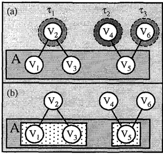
Modified Step 1: The hypergraph 7-{ associated with the given potential U is

Modified Step 2: The graph associated with the hy­ pergraph is given in Figure 3(a). Note that a new edge appears connecting vl and v3.

Modified Step 8: Since we are interested in the non­ null interaction functions we must check whether the candidate functions are non-null.

We have the following cases:

Case 1: The interaction function in v1 and v3 becomes null:

which implies

Thus, Case 1 refers to the family of Gibbs models sat­ isfying (19).

Then we have

Case 2: Otherwise, since the potential U restricted to A is { et13v1 V3 } , the potential U A becomes

Modified Step 9: The marginal hypergmph becomes:

Modified Step 10: Finally, the associated marginal gmph is

Let 9'Aa and Q(HA) be the marginal graph (algorithm 1) , and the graph associated with the marginal hy­ pergraph (algorithm 2), for the subset of variables A, respectively. Then, from Examples 5 and 6 we can conclude:

1. In case the edge (V1, V3) is not in 9 = Q('H), then (VI, V3) is an edge of both 9'Aa and Q('H A )·
2. In case the edge ( V I, V3) is in 9 = 9(H), then (V1, V3) is an edge of 9'Aa, but, if condition (19) applies, it is not and edge of 9(H A ).

The absence of ( VI, V3) as an edge of a graph over A = {Vr, V 3, 115 } implies the stochastic independence of both variables conditioned to V5. This independence statement is included in the model which has ( VI, V3) as an edge of Q(H) and verifies (19) . This shows that, in this case, the undirected graph representation of the model is not able to capture this separating statement while the hypergraph model is.

5 EXAMPLE OF APPLICATION

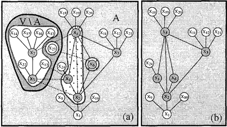
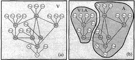
In this example, the objective is to assess the damage of reinforced concrete structures of buildings. This ex­ ample, which is taken from Liu and Li (1994) (see also Castillo, Gutierrez, and Hadi (1997) ) , is slightly mod­ ified for illustrative purposes. The goal variable (the damage of a reinforced concrete beam) is denoted by X I· A civil engineer initially identifies 16 variables (Xg, . . . , X24) as the main variables influencing the damage of reinforced concrete structures. In addition, the engineer identifies seven intermediate unobservable variables (X2, · · . , X8) that define some partial states of the structure. Table 1 shows the list of variables and their definitions.

In our example, the engineer specifies the following cause-effect relationships, as depicted in Figure 4(a) . The goal variable X I, is related primarily to three fac­ tors: X9, the weakness of the beam available in the form of a damage factor; X10, the deflection of the beam; and X2, its cracking state. The cracking state,

X 1.	Definition
XI	Damage assessment
x2	Cracking state Cracking state in shear domain Steel corrosion Cracking state in flexure
x3
x4
Xs	domain
x6	Shrinkage cracking
x7	Worst cracking in flexure domain
Xs	Corrosion state

• Xg Weakness of the beam
• x10 Deflection of the beam
• xi2 Breadth of the worst shear crack
• Xu Position of the worst shear crack
• xi3 Position of the worst flexure crack
• X14 Breadth of the worst flexure crack
• X1s Length of the worst flexure cracks
• X11 Structure age
• xl6 Cover
• XIs Humidity
• X19 PH value in the air
• X2o Content of chlorine in the air
• X22 Number of flexure cracks
• X21 Number of shear cracks
• X23 Shrinkage
• X24 Corrosion

Table 1: Definitions of the variables related to damage assessment of reinforced concrete structures.

x2, is related to four variables: x3, the cracking state in the shear domain; X6, the evaluation of the shrink­ age cracking; X4, the evaluation of the steel corro­ sion; and X5, the cracking state in the flexure domain. Shrinkage cracking, XG, is related to shrinkage, x23, and the corrosion state, X8. Steel corrosion, X4, is related to X8, X24, and X5. The cracking state in the shear domain, X3, is related to four factors: Xu, the position of the worst shear crack; xl2, the breadth of the worst shear crack; X21, the number of shear cracks; and Xs. The cracking state in the flexure domain, X5 is affected by three variables: XI3> the position of the worst flexure crack; X22, the number of flexure cracks; and X7, the worst cracking state in the flexure domain. The variable X13 is influenced by X4. The variable X7 is a function of five variables: x14, the breadth of the worst flexure crack; X15, the length of the worst flex­ ure crack; X 16, the cover; X 17, the structure age; and Xs, the corrosion state. The variable X8 is related to three variables: X18, the humidity; XI9, the PH value in the air; and X2o, the content of chlorine in the air.

A graphical representation of the damage problem is shown in Figure 4( a) .

Suppose that we are interested in suppressing all the nodes related to the flexion of the beam and keep the remaining nodes (Set A), that is (see Figure 4(b)):

5.1 GRAPH APPROACH

In this case, to marginalize over A, we can apply Al­ gorithm 1.

Step 1: The set E\ A , that is, the set of edges in the subgraph Q A is shown in Figure 4 ( b ) (the continuous edges in the region A).

Step 2: The subgraph 9v\A appears in Figure 4 ( b ) (region A with continuous edges) .

Step 3: The connectivity components T of 9v\A:

are shown in Figure 5(a) as white regions.

Step 4: The boundaries of the two connectivity com­ ponents are bd(Tl) = {Xz, x4, Xs} and bd(Tz) = {X6}, as shown in Figure 5(a) where they have been shad­ owed with dots.

Step 5: To complete the set bd( Tl) we need to add the edge (X2, X8) to the already two existing edges

(Xz, X4) and (X4, Xs).

Step 6: We return the graph in Figure 5(b) , which incorporates the edge (X2, X8) to the subgraph Q A , thus, showing that the graph A is not collapsible with respect to A. I

5.2 HYPERGRAPH APPROACH

When applying algorithm 2, the differences with the preceding results could only appear in the bound­ aries of the connectivity components of V \ A, that. is, bd(Tl) = {Xz, X4, Xs} and bd(Tz) = {XG}. The non-null innovations (13) could only arise for subsets of variables contained in these sets. As bd( Tz) has only one variable, our problem of exploring possible differ­ ences between QAw and Q('H A ) reduce to those edges connecting variables in bd( T1).

To illustrate, let us assume a Gaussian distribution with mean f1 and dispersion matrix 2: for the 24 vari­ ables in V. To express this distribution as a hypergraph model, it is easier to work with the precision matrix Y = 2:1 . In fact its pdf can be written as

corresponding to expression ( 1) with normalized po­ tential. Equation (20) shows the relationship between edges in Q and non null elements of the matrix Y.

It is a well known fact. that the marginal distribution of a multivariate Gaussian model is again multivariate Gaussian, with precision matrix

where the subscripts of Y stand for the appropriate partition.

Equation (21) shows the decomposition of the preci­ sion matrix y A related to the marginal normalized po­ tential U A in two components:

• (i) the matrix Y A , A corresponding to the restricted potential U\ A , and
• (ii) the matrix f A = Y A ,V\ A (YV\ A ,V\ A )1 Yv\A,A corresponding to innovations V f (b) of ( 13).

In particular, the innovation (13) for two variables Vi and Yj in A is

where Prs stands for the rs-element of matrix (Yv\A ,V\ A )- 1 and i rv r indicates that node i is di­ rectly connected to node r in the associated graph Q.

Particularizing to our example, the only edges sub­ ject to change when applying Algorithm 2 are {(Xz,X4), (Xz, Xs), (X4, Xs)}.

The edge (X2, X8), which was not present in the orig­ inal graph Q, arises as a consequence of the innovation [�8 = P5.7 12,51 7.8, and it is null only if (J;,.7 vanishes. iviatrix 1, being a precision matrix, is definite posi­ tive, implying D = 1 1 V \ A. V \ A I > 0. After some alge­ bra, P5,7 can be written as

113,13114,14115.15116.16117,17122.2212,515,717,8/ which cannot be null unless one or more of the pa­ rameteres 1 2,5, 15,7 and 17,8 contradict the initial specification of Q. (X2, X8) will always be present in gAw and Q(1iA)·

Conditions for (X2, X4) and (X4, X8) Q('HA) are = f2.4 and 14.8 =

D vanish. But this would Then, the edge to disappear in 12,4 f4.8 , respectively.

They state functional relationships between the pa­ rameters 12,4, 14,8 and those in 1 V \ A, V \ A. These relationships are compatible with the initial graph Q. Thus, the marginal graphs QA'a and Q(HA) could dif­ fer in edges (X2, X4) and (X4, X8), according to these conditions.

Thus, the example illustrates clearly the advantages of hypergraph models over the usual graph models.

6 CONCLUSIONS AND RECOMMENDATIONS

Hypergraph models have been shown to be a power­ ful alternative to undirected graph models. The main advantage consists of its capability to produce finer factorizations and to catch a more complete set of con­ ditional independence statements. Given a set of vari­ ables and an undirected graph or hypergraph model, two algorithms have been given for obtaining the cor­ responding marginal graph and hypergraph, such that the marginal distribution factorizes according to them. The examples have shown that in some cases the hy­ pergraph is able to capture conditional independence statements that the graph fails to detect. In addition, theorem 2 states a general framework to understand the necessary and sufficient conditions of graphical and parametric collapsibility.

Acknowledgments

The authors are grateful to Iberdrola, the U niversi­ ties of Cantabria, Jaume I and Valencia, and the Di­ reccion General de Investigacion Cientifica y Tecnica (DGICYT) (projects TIC96-0580 and PB96-0776) for partial support of this research.

References

1. Asmussen, S. and Edwards, D., (1983) . Collapsi­ bility and response variables in contingency ta­ bles. Biometrika, 70, 567-578.
2. E. Castillo, J.M. Gutierrez, and A.S. Hadi, (1997). Expert Systems and Pmbabilistic Network
3. Models. Springer Verlag, New York.
4. Darroch, J. N., Lauritzen, S. L., and Speed, T. P. (1980) , Tvlarkov Fields and Log-linear Models for Contingency Tables. Annals of Statistics, 8: 522539.
5. Frydenberg, M. (1990) , Marginalization and col­ lapsibility in graphical interaction models Annals of Statistics, 18: 790-805.
6. Isham, B. (1981), An Introduction to Spatial Point Processes and Markov Random Fields. In­ ternational Statistical Review, 49:21-43.
7. Lauritzen, S. L. (1989) , Lectures on Contingency Tables, 3rd edition. Aalborg University Press, Aalborg, Denmark.
8. Lauritzen, S.L. (1996) , Graphical Models. Oxford University Press, Oxford Statistical Science Se­ ries, Vol 17.
9. Liu, X. and Li, Z. (1994) , A Reasoning Method in Damage Assessment of Buildings. Micmcom­ puters in Civil Engineering, Special Issue on Un­ certainty in Expert Systems, 9: 329-334.
10. Mellouli, K. (1987) , On the Propagation of Belief Networks Using the Dempster-Shafer Theory of Evidence. Ph. D. Dissertation, School of Business, University of Kansas.
11. Wermuth, N. and Lauritzen, S. L. (1983) , Graphi­ cal and Recursive Models for Contingency Tables. Biometrika, 70: 537-552.
12. Pearl, J. and Paz, A. (1987) , Graphoids: A Graph-Based Logic for Reasoning about Rele­ vance Relations. In Boulay, B. D., Hogg, D., and Steels, L., editors, Advances in Artificial Intelligence-II. North Holland, Amsterdam, 357363.
13. Rose, D. J. (1970) , Triangulated Graphs and the Elimination Process. Journal of Math. Anal. Appl. 32, 597-609.
14. Tarjan, R. and Yannakakis, M. (1984), Sim­ ple linear-time algorithms to test chordality of graphs, test acyclicity of hypergraphs, and selec­ tively reduce acyclic hypergraphs. SIAM Journal of Computing, 13(3) .
15. Sanmartin, P. (1997) , Agregacion Temporal en Modelos de Grafos Cadena. Ph. D. Thesis, Uni­ versity of Valencia.
16. Shafer, G. and Shenoy, P. (1990) , Probability Propagation. Annals of lVIathematics and Arti­ ficial Intelligence, 2: 327-352.
17. Studeny, IVI. (1994), On Marginalization, Col­ lapsibility, and precollapsibility. In V . benes, J. Stepan eds.: Distributions with Given Marginals and Moment Problems, Kluwer, Dordrecht, 191198
18. Winkler, G. (1995) , Image Analysis, Random Fields and Dynamic Monte Carlo ·Methods. A Matematical Introduction. Springer.