I

Markov Chain Monte Carlo using Tree-Based Priors on Model Structure

Nicos Angelopoulos

James Cussens

Department of Computer Science, University of York

Heslington, York, YOlO 5DD, UK {nicos,jc}®cs.york.ac.uk

Abstract

We present a general framework for defining priors on model structure and sampling from the posterior using the Metropolis-Hastings algo­ rithm. The key ideas are that structure priors are defined via a probability tree and that the pro­ posal distribution for the Metropolis-Hastings al­ gorithm is defined using the prior, thereby defin­ ing a cheaply computable acceptance probabil­ ity. We have applied this approach to Bayesian net structure learning using a number of priors and proposal distributions. Our results show that these must be chosen appropriately for this ap­ proach to be successful.

1 INTRODUCTION

This paper extends and empirically evaluates a general framework for Bayesian modelling which was briefly sketched in (Cussens, 2000). O u r primary goal is to imple­ ment a practical method of incorporating prior information about model structure. The current lack of such a method is noted by Friedman and Koller (2000) in their paper on Bayesian learning of Bayesian network structure which is closely related to this paper

. . . relatively little attention has been paid to the choice of structure prior, and a simple prior is of­ ten chosen largely for pragmatic reasons .... The standard priors over network structure are often used not because they are particularly appropri­ ate for a task, but rather because they are simple and easy to work with.

Although our approach is very general-for example, in (Cussens, 2000) it was applied to a model space com­ posed of logic programs-the experiments here are fo­ cused exclusively on learning Bayesian network (BN)

structure from data and prior knowledge. In many ap­ plications we are likely to have at least some knowledge about network structure which we are willing to model as hard constraints, for example, that X is/is not a par­ ent/child/ancestor/descendant of Y, that X andY are inde­ pendent/dependent, that no family has more than k parents, etc. We may also wish to express softer prior beliefs, for example, encoding a preference for sparsely connected net­ works. Both hard and soft prior information are expressible in our method.

2 TREE-BASED PRIORS ON MODEL STRUCTURE

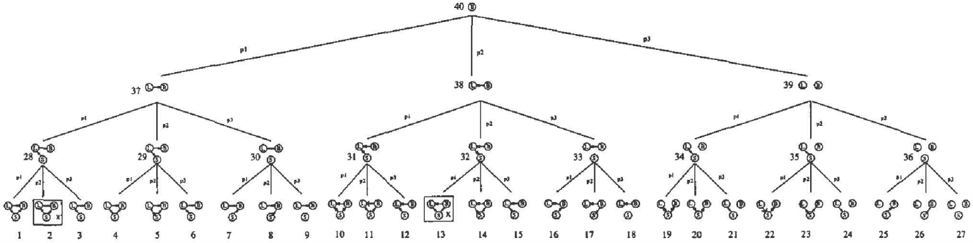
Our approach to defining priors on a finite or countably infi­ nite space of models is best understood in terms of the sam­ pling process which selects a model from the model space. The sampling process is a series of independent choices where for each choice-point there is a multinomial distribu­ tion over the choices available. Some sequences of choices are defined as successful and these determine (or yield) a model in the space. Sequences of choices can be repre­ sented as distinct branches in a probability tree. Figure 5 (see last page) presents ENTREE, an example of such a probability tree for the very small model space of all 25 Bayesian networks consisting of the random variables B, L and S. At each choice point in this tree we choose how to connect a particular pair of variables where the pairs are considered in the following order: (B, L), (L, S), (B, S) .

BNT REE is very simple in that each choice-point has the same multinomial distribution. If (X, Y) is the pair of ran­ dom variables under consideration then there is probability Pl that Y is chosen to be a parent of X, probability P2 that Y is chosen to be a child of X, and probability p3 that there is to be no direct connection between X and Y. In general, we could have many multinornials, with the Pi depending on (X, Y), thus giving a very detailed prior specification.

Two branches, or derivations as we shall now call them, in BNT REE lead to cyclic graphs at leaves 2 and 13which are not in the model space of Bayesian nets. These

一

are therefore labelled as failure derivations and correspond to failed attempts to sample a Bayesian net. If a derivation is not a failure derivation then it is a successful derivation.

ENTREE defines three probability distributions: 1/J>.., f>. and P>.. .\ denotes the log versions of the parameters, so for ENTREE,.\ = (logp1,logp2,logp3). For any derivation x, 1/J>. (x) is the product of the probabilities at­ tached to the choices that constitute x. For example if x2 is the derivation leading to leaf 2 in ENTREE, then 1/J>. (xz) = PiP2. !>. ( x ) is simply 1/J>. (xlx is successful), so:

where Z >. is the normalising constant:

From a sampling point of view, Z>-. is the probability that the next attempt at sampling will be successful. f>. is es­ sentially a log-linear distribution (also know as a Gibbs distribution, or, in the computational linguistics literature, a MAXENT distribution). To see this let the frequency Of a choice Ci in a SUCCeSsful derivation X be L'i(X), then f>.(x) = ZJ: 1 llip�· ( x ) = Z):1 exp(L:;i .\iv,(x)). In the language of log-linear modelling, the Vi are the 'features' of derivations. Here the features are integer-valued but this is not generally the case for log-linear models.

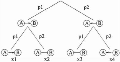
In the particular case of ENTREE there is only one derivation for each BN, so there is a bijection between mod­ els and successful derivations. In general, this is not the case. To see this, consider the probability tree CGT REE in Figure 1 which defines a distribution J>. over 4 successful derivations and a distribution, which we will call P>., over the model space which consists of 3 chain graphs. At each choice point we choose between either an edge from A to E or an edge from E to A. An undirected edge corresponds to an edge in both directions. Two derivations, x2 and X3, yield the undirected graph MA-B· We define P>. so that P>.(MA-B) = f>.(x2) + f>.( x 3) = P1P2 + P2Pl = 2PIP2· In general, P>.(M) is just the distribution over models de­ fined by marginalising derivations away:

To get a feel for the distributions defined by ENTREE, suppose we set PI = P2 = p3 = 1/3. This means Vx1/J>.(x) = 1/27. Z>. = 25/27, so f>.(x) = 1/25 for all successful x and P>. ( M ) = 1/25 for all BNs. Increasing P3 at the expense of p1 and P2 expresses a preference for sparsely connected BNs and would make BN27 (the

BN at leaf 27 in Fig 5) the mode of the prior. Setting PI = 0 almost surely removes each leftmost choice from each choice-point effectively reducing the model space to (BN14, EN1s, BN11, BN1s, ENz3, EN24, EN2s, BNz1 ) , the BNs consistent with the variable ordering (E,L,S). Setting P3 = 0 effectively reduces the model space to (BNl,EN4,EN5,BN1 0 ,BN11,BN14), the 6 totally connected BNs.

3 MCMC USING THE METROPOLIS-HASTINGS ALGORITHM

In the Bayesian approach to statistical inference we do not 'learn' or 'induce' a single best model from the data D. In­ stead a posterior distribution P(MID) is derived from the prior distribution P(M) using Bayes theorem. This poste­ rior distribution is then used to compute the expected values of various quantities of interest.

Unfortunately, we know of no way of updating the prob­ ability trees representing our· priors into (practical) trees representing posteriors. Worse still, we have no way of even sampling directly from the posterior. This is a com­ mon problem in complex Bayesian modelling and can be addressed by employing Markov chain Monte Carlo (MCMC) methods (Gilks, Richardson, & Spiegelhalter, 1996). Given a target distribution (e.g. a posterior) from which we would ideally like to sample but cannot, an MCMC algorithm constructs a Markov chain whose sta­ tionary distribution is the target distribution. If we run the chain for long enough then estimates of features of the tar­ get distribution produced by sampling this chain will con­ verge to their true values, under fairly weak conditions.

We use the Metropolis-Hastings (MH) algorithm to con­ struct a Markov chain M0, M1, M2, . · . . When the target density is a posterior P(M\D) = P(M)P(DIM)/P(D), MH is defined as follows (where the initial model M0 is sampled from the prior).

1. Generate a candidate value M* with proposal proba­ bility distribution q(Mi, M*).

• point and repeat step 2, or with probability 1 -Pb go to step 3.
• Once we have stopped backtracking choose a new leaf M* f r o m the choice point by selecting branches ac­ cording to their probabilities attached to them. How­ ever, in the first step down the tree we may not choose the branch that leads back to Mi.

As long as the Markov chain is ergodic (Gilks et a!., 1996), the proposal distribution q can have any form and the sta­ tionary distribution will be P(MJD).

4 CHOOSING A PROPOSAL DISTRIBUTION FOR TREE-BASED PRIORS

Our proposal mechanism uses the same probability tree that we used to define the prior. We use MH to construct a Markov chain of derivations with stationary distribution fA(xJD). This gets us to our target posterior distribu­ tion P>.(MJD) by marginalisation similarly to (1). In our MCMC samples, we do not even record which derivation we are visiting, just the model associated with it. (F a i l ure derivations never appear in the Markov chain.) Given this close connection between f>..(xJD) andp>.(MJD) we will switch freely between talking about sequences of deriva­ tions and sequences of models.

The basic idea is to 'bounce' around the tree by backtrack­ ing from the current leaf to an interior node and then going down the tree to a new leaf by choosing branches using the probabilities which define the prior distribution. Note that there is a one-one correspondence between leaves and derivations, so we can describe the algorithm in terms of visiting leaves. The only caveat is that when we stop back­ tracking we may not choose the branch up which we have just backtracked-such branches are temporarily blocked. This ensures that there is a unique path between any two leaves. Using the prior distribution to construct the pro­ posal distribution is also done in (Philps & Smith, 1996; Chipman, George, & McCulloch, 1998; Denison, Mallick, & Smith, 1998) and has the advantage that many of the terms in (2) cancel out. In particular the Z>. normalising constant, which is particularly difficult to compute for large trees, disappears.

Our proposal distribution is parameterised by a backtrack probability Pb which controls the sizes of jumps. A can­ didate leaf M* is generated from a current leaf Mi as fol­ lows.

1. Backtrack one step to the most recent choice point in the probability tree.
2. We then probabilistically backtrack as follows: If at the top of the tree go to step 3. Otherwise with prob­ ability Pb backtrack one more step to the next choice

To illustrate this, consider some leaf pairs in BNT REE (the numbers refer to nodes in BNT REE):

Each proposal probability has three factors (separated by '.' above): a backtrack factor, a factor from the prior and a factor for the temporarily blocked branch.

To define the acceptance probability o:(Mi, M* ) we need some more notation. Let Mi have depth ni and M* depth n*. Let N o d e ( M i , M*) be the deepest common ancestor of Mi and M*, this is the internal node we reach when we stop backtracking from Mi. Let Ci be the choice from Node(Mi, M*) that leads to Mi, and define C* analo­ gously. Let p i and p* be the probabilities attached to Ci and C*, respectively. Then, as proven in (Cussens, 2000), if M* is a leaf at the end of a successful derivation:

If M* is a failure (for example, BN2 or BN13 in ENTREE) then o:(Mi, M*) = 0.

It is easy to see that our Markov chain is ergodic, i.e. pos­ itive recurrent and aperiodic. (See (Roberts, 1996) for the basic definitions and theorems regarding ergodicity.) For any leaves M; and Mi, it is clear that the probability P;i ( t) of moving from M; to Mi in t steps, is positive, for all t > 0. So a fortiori the Markov chain is irreducible and, since we are doing MCMC, also positive recurrent. The chain is also obviously aperiodic and so we have ergodic­ ity.

5 BAYES FACTORS FOR BAYESIAN NETS

The data only affects MH via the quantity P(DJM*)/ P(DJMi) the ratio of marginal likelihoods for

二

the proposed and current model. This ratio is known as a Bayes factor. In all but deterministic non-probabilistic models the full likelihood requires not just a determination of model structure but also of the model parameters. In the case of a BN network structure M, these are the conditional probability distributions () x, ]u, for the random variables Xi and each instantiation u; of their parents PaM(X;). To calculate the Bayes factor we need to marginalise away (i.e. integrate away) these model parameters.

Here we make the standard assumptions to allow this inte­ gration to have a closed form. Firstly, we assume a Dirich­ let prior over () x, 1 u ; for all X; and u;. We also assume global parameter independence and parameter modular­ ity. The former says that the total de n sity over the com­ plete parameter set is the product of the individual Ox,]u; densities and the latter that Bx; �u ; is the same for any two network structures where Xi has the same parents. Our fi­ nal assumption is that the data is complete, each data point contains an observation for each random variable.

Given all these convenient assumptions we have from (Heckerman, 1996) that the marginal likelihood is a prod­ uct of 'scores' for each family in the BN M:

Let N;jk be the count in the data for X; taking value k when its parents have instantiation j. Let a;jk be the corre­ sponding Dirichlet parameter. Let Do m (Xi ) be set of pos­ sible values of X;. Define N ;j = L: kEDom(X;) Niik and a;i = L:kEDom(X;) Gijk· Then score(X;, PaM(X;)JD) is

If Xi has the same parents in Mi and M· then the score for X; cancels out in the Bayes factor making it quick to compute the Bayes factor for similar BNs. We also cache scores. All our computations are done by taking logs and using the log r function from the c maths library. Everything else is done in Prolog including the definition of the Oijk. Setting the Gijk to informative values ex­ presses prior knowledge about likely conditional probabil­ ity values, but in our current artificial experiments we set Gijk = 1, Vi,j, k.

6 DEFINING TREE-BASED PRIORS USING STOCHASTIC LOGIC PROGRAMS

Our tree-based MCMC approach is implemented using stochastic logic programs (SLPs). This is because the logic

bn( [], [], []). bn([RVjRVs] ,BN,AncBN) bn(RVs,BN2,AncBN2), connect_no_cycles(RV,BN2,AncBN2,BN,AncBN). %RV parent of H, p_l=l/3 1/3 :: which edge( [H]T] ,RV, [H-RV]Rest]) choose edges(T,RV,Rest). tRV child of H, p 2=1/3 l/3 :: which edgel[H]TI ,RV, [RV-H!Rest]) choose edges(T,RV,Reat). \no edge� p_3=1/3 l/3 :: which edge([ HjT] ,RV,Rest) choose_edges(T,RV�Rest).

progr amm ing paradigm gives us a number of facilities for free:

1. Easy declarative representation of the model space and constraints on models using a subset of first-order logic;
2. Implicit definition of the tree structure (by a logic pro­ gram and goal);
3. Automatic construction of models as we move down the tree (building first-order terms via successive uni­ fications;
4. Backtracking concepts which could be extended to in­ corporate sampling over SLPs;
5. A built-in notion of failure (unification failure).

In most of our experiments we used variants of the prior defined by the SLP SEN in Fig 2. The predicate bn/3 in Fig 2 says that EN is a Bayesian net constructed from the variables in the list [RV I RVs] if BN2 is a Bayesian net constructed from the list RVs and RV is connected to BN2 without introducing any cycles. The Prolog operator ':-' should be read as ·�·. BNs are represented as ordered lists of families, for example BNs is represented as [b­ [ l] , l-[] , s[b) ) . This is a natural representation and one that allows us to use utility predicates from the Sics­ tus Pro log ugraphs library. The third argument in bn/ 3 represents the ancestor sets for each node, so for BNs it would be [b- [1] , 1- [] , s[b,l]]. The ancestor sets allow quick checking for cycles and allow us to easily put constraints on ancestor relationships.

A logic program P together with a goal G, defines an SLD­ tree each branch of which is a refutation of G using P. For example, given the SLP SEN parts of which are given in Fig 2 and the goal VBN-..,bn([s,l,b],BN) ("there are no ENs with s, l and b as nodes") we (essentially) get BNT REE as an SLD-tree. Each successful branch re­ futes our goal and provides an instantiation of BN as a counterexample. In other words, each branch is a construc­ tive proof that there exists a particular B N.

It is important to understand that the SLD-tree is never ac­ tually constructed, it is just a representation of Prolog's search space (standard Prolog explores it deterministically: depth-first, leftmost-first). This means we can define very large, even infinite trees, with a logic program.

To define a prior over models using an SLP, one takes a logic program P and associates probabilities with some of the clauses in the logic program. For example, in SBN the three clauses defining which_ edge/ 3 are the only prob­ abilistic ones. Denote the resulting SLP by S and let the (logs of) the probabilities added be>. = (>.1, >.2, . . . , An). For any goal G, S has an associated SLD-tree: the one for its underlying logic program P. Each choice in the SLD­ tree is associated with a choice of clause, so some choices will have associated probabilities. Construct a probability tree by deleting all choices from the SLD-tree which have no associated probability. The SLP defines three distribu­ tions 1/J(>. , S , G)· !(>. , S , G) and P(>.,S , G) (usually abbreviated to 1/J>., f>. and P>.) via this probability tree exactly as de­ scribed in Section 2. For a more detailed account of how SLPs define distributions see (Cussens, 2001).

7 EXPERIMENTS

7.1 A PRELIM:INARY EXPERIMENT

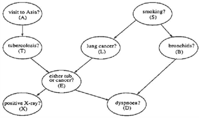
For our first experiment we sampled 10,000 data points from the 3-node BN constructed from the S, LandE nodes of the well-known 'Asia' network given in Fig 3. This is BN19 in Fig 5. We then used a uniform prior over the set of 25 BNs with three nodes and did MCMC as described above with 106 iterations and a burn-in of 5000. The results are in Table 1. The BNs in Table 1 fall into two Markov equivalence classes divided by a horizontal line. Note that the BN that generated the data (ENt9) has much lower pos­ terior probability than EN22· Although the posterior prob­ abilities estimated by MCMC are eventually close to the true values, convergence is very slow.

Table 1: Estimated Cfti) and actual (p) posterior probabili­ ties for the nine most probable 3-node BNs in ENTREE rounded to 3 d.p. Pi is the estimated probability after lQi iterations. The other sixteen highly improbable BNs were never visited, so for them Vi : Pi = 0.

M	P4			p
	0.668	0.690	0.704	0.702
	0.176	0.150	0.145	0.146
	0.144	0.152	0.143	0.145
EN4	0.007	0.005	0.005	0.005
ENs	0.002	0.001	0.002	0.002
EN1	0.001	0.001	0.001	0.001
EN14	0	0	0	0
ENw	0.001	0	0	0
ENn	0	0	0	0

7.2 IMPROVING MCMC

To address the issue of slow convergence and hence pro­ duce reasonable estimates in bigger model spaces we made a number of improvements over the basic approach de­ scribed above. One of the key issues in MCMC is to strike a balance between local jumps to 'neighbouring' candi­ date models and big jumps to distant ones. With a bias towards local jumps there is a risk that the chain will re­ main stuck in a particular neighbourhood, perhaps failing to visit areas of high posterior probability. This is less of a problem if we can move a big distance via a sequence of local jumps. Unfortunately, this is not the case with the trees, such as BNT REE, associated with priors defined by S8N in Fig 2. Since all the leaves are of equal depth (this depth is 28 for the 8-node BN model space) we can only reach a leaf on the 'other side' of the root node by do­ ing one big jump via this root node-there are no shallower leaves that can help us reach the root node by a sequence of small jumps. Even with Pb = 0.98 our chains get stuck, very rarely proposing distant candidates and rejecting them when they are proposed.

Solving this problem by going for big jumps brings its own problems. Sooner or later the chain should find its way to a model with a posterior probability higher than the vast ma­ jority of other models, including the vast majority of dis­ tant models. This will mean that many candidate models will be rejected-the chain will be stuck-unable to find other models of high posterior probability from amongst the mass of low probability models. Indeed, the rationale for local jumps is that we should give ourselves the oppor­ tunity to visit neighbouring models, since if a model has high probability then maybe so will many of its neighbours, since they are, in some way, similar.

In our approach the neighbourhoods are defined by the topology of the tree, and the distance between them is regulated by Pb· the backtrack probability. We effect a

二

compromise between local and big jumps by implement­ ing a cyclic transition kernel. We cycle through the values Pb == 1 -z-n, for n == 1, . . . , 28, so that on every 28th iteration, there is a high probability of backtracking all the way to the top of the tree.

We have also found it effective where possible to manually re-write our SLPs so that they are failure-free. If there are lots of failure points in the probability/SLD tree, then many candidates will be failures. Since we never jump to a fail­ ure leaf this can lead to poor mixing, particularly when we include many constraints so that successful branches are surrounded by many failures.

7.3 RESULTS

We generated 2295 data points from the entire 'Asia' BN and constructed Markov chains over the space of all 8node BNs. There are 783,702,329,343 BNs in this model space. Firstly we used an SLP which defined a prior over all 8-node BNs consistent with a particular variable order­ ing (one consistent with the 'Asia' BN). We also did experi­ ments with the added constraints that the number of parents for a node is limited to k == 2 and k = 3. The first-order framework makes it easy to add constraints. However care is needed to write SLP priors which allow reasonable con­ vergence.

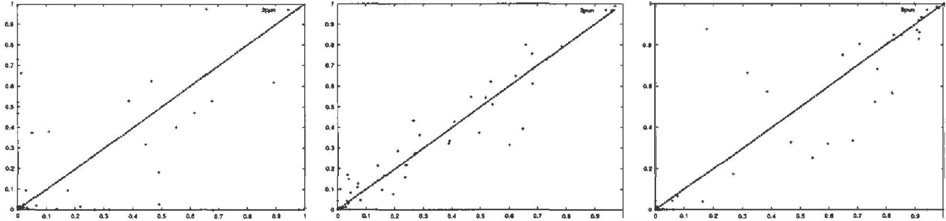
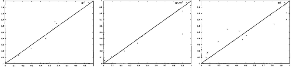
For each setting of the constraints, we did two runs each of 500,000 iterations. We then used the sample so created to estimate the posterior probability that xi is a parent of Xi for all i, j consistent with the ordering. There are 28 of these features. Plotting the estimates from the two runs against each other produced the results in Fig 6. In Fig 6 we also have results when only half of the data was used (1124 data points). We then ran the same set of experiments but did not impose an ordering on the variables, and in one case removed the limit on the number of parents. The results of these experiments are in Fig 7. For each pair of runs, Figs 6 and 7 contain runtimes in seconds for a Pentium III I GHz running SICStus 3.8.5 under Linux.

Ideally, all points in Figs 6 and 7 would be on the diago­ nal, showing that estimates produced from the two different runs were equal. Basically, we get points near the diagonal if either the estimates are near 0 or 1 (there are lots of these and they are not easily visible on the plots) or the model space is constrained, particularly if constrained by an or­ dering. In the totally unrestricted case (rightmost plot of Fig 7), we get a few really bad points. In the worst case A was almost always the parent of D in the first run, but this was almost never the case in the second. These results fit our expectations, the "near 0 or 1" phenomenon follows from basic sampling theory, and it is no surprise that esti­ mates are more reliable in constrained settings. One sur­ prise is that we expected better results using only half the data, since then the shape of the posterior is less spiky, how- ever the results are essentially the same.

To see whether we could use the child-parent probability estimates to get a partial picture of the 'true' BN we con­ structed a BN where there was a link from Xi to Xi when­ ever that link had estimated probability greater than 95%. We did this for (i) the totally unconstrained case, (ii) when only a maximum of k = 3 parents were allowed and (iii) when only a maximum of k = 3 parents were allowed, but the parents of E were forced to be T and L. This last con­ straint seems reasonable since E is defined to be "either Tor L". The resulting BNs are Fig 8. As expected, we get spurious links in the unconstrained case with A and T parents of B, even though A and T are marginally inde­ pendent of B in the data generating 'Asia' network. For the two cases with k = 3 constraints on the parents, we get no links that are not in 'Asia'. It is surprising that we never have either ofT or L the parent of E even though E is a function ofT and L.

8 DISCUSSION

Friedman and Koller (2000) state that "different runs of MCMC over networks lead to very different estimates in the posterior probabilities of structural features". Although a number of our experiments have this problem it is not always the case (although, unlike Friedman and Koller (2000), we have yet to work with variable sets as large as 37). The consistency of the probability estimates depends on how constrained the model space is (as well as how well designed our MCMC strategy is). The stronger our prior knowledge the better the estimates. We see our main con­ tribution as providing a framework for incorporating prior knowledge in a declarative and practical manner. One ad­ vantage of working directly on network structure is that it makes it easier to actually write down the sort of prior knowledge we might have.

It is instructive to compare our approach with the Markov chain Monte Carlo model composition (MC 3 ) approach in­ troduced by Madigan and York ( 1995). The MC 3 algorithm moves through the model space by altering only one edge at a time. The proposal distribution is not based upon the prior, and so the ratio of the priors of the current and pro­ posed models is computed to find the acceptance probabil­ ity, in contrast to our (3). Priors are used where this ratio is easily found and MC 3 has been successfully applied to a number of datasets.

Madigan, Andersson, Perlman, and Volinsky (1996) point out that there are strong computational and statistical ar­ guments in favour of using a model space each element of which is a Markov-equivalence class of BNs, rather than a single BN. Surprisingly, each class has on average only about 4 members-a significant proportion have only one member (Gillespie & Perlman, 2001). Each Markov­ equivalence class [D] is uniquely represented by a unique

chain graph D*, the essential graph. It is easy to de­ fine a prior over essential graphs and hence over Markov­ equivalence classes using an SLP. These can be extended to define a prior over BNs if desired. SEa, a fragment of which is given in Fig 4, does this and is most eas­ ily understood by looking at the steps used to sample from the prior it defines. Given a set of random variables RVs, skeleton/2 first probabilistically chooses an undi­ rected graph Skel, then essential_graph/3 proba­ bilistically chooses an essential graph EG with immoralities Imms by adding arrows to Skel. bn/3 is then defined to probabilistically choose a particular BN from the equiva­ lence class of BNs defined by EG. It is more natural to de­ fine a prior over essential graphs, but we extended the prior to be over BNs to compare with our previous experiments.

bn(RVs,BN) :-skeleton(RVs,Skel), essential_graph(Skel,Imms,EG), bn (EG, Imms,BN), top _ sort(BN,_). %check for cycles

Although it was easy to define the prior, the associated probability tree had far too many failure derivations to be useful. A similar problem occurred when, in a sepa­ rate experiment, we used a prior with constraints enforcing marginal independence between pairs of nodes.

Although all the experiments here are for BNs our approach is general. Our SLP implementation, which works by trans­ lating a human-readable SLP as in Fig 2 to Prolog, does not 'know' that the first-order terms are BNs. If we want to apply our method to different models, we just write the appropriate SLP priors and write code to compute the ap­ propriate Bayes factors.

Our final conclusion is that further work is required to fully understand the advantages and limitations of our approach. There are many methods in the literature for improving MCMC and we have only tried one of them (the use of a cyclic transition kernel). One big problem was that natural ways of defining priors generally led to inefficient MCMC due to the existence of many failures. The same problem arises in logic programming where it is addressed using source-to-source program transformation. We expect pro­ gram transformation to be necessary for real applications, where, if we can exploit prior information using our frame­ work, substantial benefits are possible.

Acknowledgements

This work was supported by EPSRC research grant GR/N09152 Induction of Stochastic Logic Programs. Many thanks to our four anonymous reviewers for their in­ sightful criticisms of a previous version of this paper.

References

• Chipman, H. A., George, E. 1., & McCulloch, R. E. (1998). Bayesian CART model search. Journal of the Amer­ ican Statistical Association, 39(443), 935-960. With discussion.
• Cussens, J. (2000). Stochastic logic programs: Sampling, inference and applications. In Proceedings of the Six­ teenth Annual Conference on Uncertainty in Artifi­ cial Intelligence (UAI-2000), pp. 115-122 San Fran­ cisco, CA. Morgan Kaufmann.
• Cussens, J. (2001). Parameter estimation in stochastic logic programs. Machine Learning, 44(3), 245-271.

Denison, D. G. T., Mallick, B. K., & Smith, A. F. M. (1998). A Bayesian CART algorithm. Biometrika, 85(2), 363-377.

• Friedman, N., & Koller, D. (2000). Being Bayesian about network structure. In Uncertainty in Artificial In­ telligence: Proceedings of the Sixteenth Conference (UAI-2000), pp. 201-210 San Francisco, CA. Mor­ gan Kaufmann Publishers.
• Gilks, W. R., Richardson, S., & Spiegelhalter, D. (Eds.). (1996). Markov Chain Monte Carlo in Practice. Chapman & Hall, London.
• Gillespie, S. B., & Perlman, M. D. (2001). Enumerating Markov equivalence classes of acyclic digraph mod­ els. In Uncertainty in Artificial Intelligence: Pro­ ceedings of the Seventeenth Conference (UAI-2001) San Francisco, CA. Morgan Kaufmann Publishers.
• Heckerman, D. (1996). A tutorial on learning with Bayesian networks. Tech. rep. MSR-TR-95-06, Mi­ crosoft Research.
• Madigan, D., Andersson, S. A., Perlman, M. D., & Volin­ sky, C. T. (1996). Bayesian model averaging and model selection for Markov equivalence classes of acycic digraphs. Communications in Statistics: The­ ory and Methods, 25, 2493-2520.
• Madigan, D., & York, J. (1995). Bayesian graphical models for discrete data. International Statistical Review, 63, 215-232.
• Philps, D. B., & Smith, A. F. M. (1996). Bayesian model comparison via jump diffusions. In Gilks, W. R., Richardson, S., & Spiegelhalter, D. (Eds.), Markov Chain Monte Carlo in Practice, pp. 215-240. Chap­ man & Hall, London.
• Roberts, G. 0. (1996). Markov chain concepts related to sampling algorithms. In Gilks, W. R., Richardson, S., & Spiegelhalter, D. (Eds.), Markov Chain Monte Carlo in Practice, pp. 45-57. Chapman & Hall, Lon­ don.

.