Mini-Bucket Heuristics for Improved Search

Kalev Kask and Rina Dechter

Department of Information and Computer Science University of California, Irvine, CA 92697-3425 {kkask,dechter }@ics.uci.edu

Abstract

The paper is a second in a series of two pa­ pers evaluating the power of a new scheme that generates search heuristics mechanically. The heuristics are extracted from an approx­ imation scheme called mini-bucket elimina­ tion that was recently introduced. The first paper introduced the idea and evaluated it within Branch-and-Bound search. In the cur­ rent paper the idea is further extended and evaluated within Best-First search. The re­ sulting algorithms are compared on coding and medical diagnosis problems, using vary­ ing strength of the mini-bucket heuristics.

Our results demonstrate an effective search scheme that permits controlled tradeoff be­ tween preprocessing (for heuristic genera­ tion) and search. Best-first search is shown to outperform Branch-and-Bound, when sup­ plied with good heuristics, and sufficient memory space.

1 Introduction

The paper is a second in a series of two papers eval­ uating the power of a new scheme that generates search heuristics mechanically. In the first paper [Kask and Dechter, 1999a], we proposed a new scheme that uses the mini-bucket approximation methods to generate heuristics for search algorithms. Since the mini-bucket's approximation accuracy is controlled by a bounding parameter, it allows heuristics having vary­ ing degrees of accuracy and results in a spectrum of search algorithms that can tradeoff heuristic compu­ tation and search.

The idea was studied using a branch and bound search for finding the most probable explanation (MPE) in Bayesian networks. Empirical evaluations demon­ strated good performance, superior to algorithms such as bucket elimination or join-tree clustering, while im­ proving on mini-bucket approximations.

In the current paper we explore the power of the mini­ bucket heuristics within Best-First search. Since, as shown these heuristics are admissible and monotonic, , their use within Best-First search yields A* type al­ gorithms whose properties are well understood; the algorithm is guaranteed to terminate with an optimal solution; when provided with more powerful heuris­ tics it explores a smaller search space, but otherwise it requires substantial space. It is also known that Best­ First algorithms are optimal. Namely, when given the same heuristic information, Best-First search is the most efficient algorithm in terms of the size of the search space it explores [Dechter and Pearl, 1985]. In particular, Branch-and-Bound will expand any node that is expanded by Best-First (up to some tie break­ ing conditions) and, in many cases it explores a larger space. Still, Best-First may occasionally fail because of its memory requirements.

The question we investigate here is to what extent the mini-bucket heuristics can facilitate the solution of larger and harder problems by Best-First search, and how Best-First is compared with Branch-and-Bound, when both have access to the same heuristic informa­ tion.

Mini-bucket is a class of parameterized approximation algorithms based on the bucket-elimination framework [Dechter, 1996]. The approximation uses a controlling parameter which allows adjustable levels of accuracy and efficiency [Dechter and Rish, 1997]. The algo­ rithms were presented and analyzed for deterministic and probabilistic tasks such as finding the most prob­ able explanation ( M P E), belief updating and finding the maximum a posteriori hypothesis. Encouraging empirical results were reported on randomly gener­ ated noisy-or networks, on medical-diagnosis CPCS networks, and on coding problems [Rish et al., 1998]. In some cases however the approximation is seriously suboptimal even when using the highest feasible accu-

M

二

racy level. This can be determined by an error bound produced by the mini-bucket scheme.

Branch-and-Bound searches the space of partial as­ signments in a depth-first manner. It will expand a partial assignment only if its upper-bounding heuris­ tic function is larger than the currently known lower bound solution. The virtue of branch-and-bound is that it requires a limited amount of memory and can be used as an anytime scheme; whenever interrupted, branch-and-bound outputs the best solution found so far. Best- First explores the search space in uniform frontiers of partial instantiations, each having the same value for the evaluation functions, while progressing in waves of decreasing values.

In this paper, a Best-First algorithm with Mini-Bucket heuristics ( BFMB) is evaluated empirically and com­ pared with a Branch and Bound algorithm using Mini­ Bucket heuristics ( BBMB), with mini-bucket approx­ imation scheme and with iterative belief propagation, over test problems such as coding networks, noisy-or networks and CPCS networks.

We show that Best-First frequently outperforms Branch and Bound, whenever Best-First terminates. Namely, when the heuristics were strong enough, if given enough time and when memory problems were not encountered. Both search methods exploit heuris­ tics strength in a similar manner; on all problem classes, the optimal tradeoff point between heuristic generation and search lies in an intermediate range of the heuristics' strength. This optimal point gradually increases towards stronger heuristics, as problems be­ come larger and harder.

Section 2 provides preliminaries and background on the mini-bucket algorithms. Section 3 describes the heuristic function which is built on top of the mini­ bucket algorithm, proves its properties and embbed the heuristic within Best-First search. Section 4 presents empirical evaluations while section 5 provides discussion and conclusions.

1.1 Related work

Our approach applies the paradigm that heuristics can be generated by consulting relaxed models, suggested in [Pearl, 1984]. The mini-bucket heuristics can also be viewed as an extension of bounded constraint prop­ agation algorithms that were investigated in the con­ straint community in the last decade [Dechter, 1992].

Here is some related work for finding the most prob­ able explanation in Bayesian networks. It is known that solving the MPE task is NP-hard. Complete algo­ rithms for MPE use either the cycle cutset ( also called conditioning) technique or the join-tree-clustering

technique [Pearl, 1988] or bucket-elimination scheme [Dechter, 1996]. However, these methods work well only if the network is sparse enough to allow small cutsets or small clusters. Following Pearl's stochastic simulation algorithms for the MPE task [Pearl, 1988], the suitability of Stochastic Local Search ( SLS) algo­ rithms for MPE was studied in the context of med­ ical diagnosis applications [Peng and Reggia, 1989] and more recently in [Kask and Dechter, 1999b]. Best first search algorithms were also proposed in [Shimony and Charniak, 1991] as well as algorithms based on linear programming [Santos, 1991].

2 Background

2.1 Notation and definitions

Belief Networks provide a formalism for reasoning about partial beliefs under conditions of uncertainty. They are defined by a directed acyclic graph over nodes representing random variables of interest.

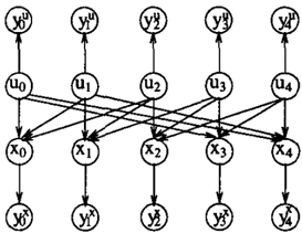
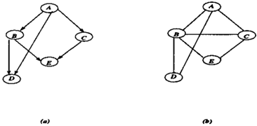
DEFINITION 2.1 (Belief Networks) Given a set, X = {Xt, ... , Xn} oj random variables over mul­ tivalued domains Dt, . . . , Dn, a belief network is a pair ( G, P) where G is a directed acyclic graph and P = {P;}. P; = {P(X; I pa (X;))} are condi­ tional probability matrices associated with X;. The set pa(X;) is called the parent set of X;. An assign­ ment (Xt = Xt, ... , Xn = Xn) can be abbreviated to x = (xt, ... , xn)· The BN represents a probability dis­ tribution P(xt, .... , Xn) = Il?=1P(x;lxpa(X;)), where, xs is the projection of x over a subset S. An evi­ dence set e is an instantiated subset of variables. The argument set of a f unction h are denoted S(h) . An example of a belief network is given in Figure 1.

DEFINITION 2.2 (Most Probable Explanation) Given a belief network and evidence e, the Most Prob­ able Explanation (MPE) task is to find an assignment (x!, . . . , x�) such that

DEFINITION 2.3 (graph concepts) An ordered graph is a pair ( G, d) where G is an undi­ rected graph and d = X1, ... , Xn is an ordering of the nodes. The width of a node in an ordered graph is the number of its earlier neighbors. The width of an or­ dering d, w(d), is the maximum width over all nodes. The induced width of an ordered graph, w* (d), is the width of the induced ordered graph obtained by process­ ing the nodes recursively, f rom last to first; when node X is processed, all its earlier neighbors are connected. The moral graph of a directed graph G is the undi­ rected graph obtained by connecting the parents of all the nodes in G and then removing the arrows.

2.2 Bucket and mini-bucket algorithms

Bucket elimination is a unifying algorithmic frame­ work for dynamic-programming algorithms appli­ cable to probabilistic and deterministic reasoning [Bertele and Brioschi, 1972, Dechter, 1996). The in­ put to a bucket-elimination algorithm consists of a col­ lection of functions or relations (e.g., clauses for propo­ sitional satisfiability, constraints, or conditional prob­ ability matrices for belief networks ) . Given a vari­ able ordering, the algorithm partitions the functions into buckets, each associated with a single variable. A function is placed in the bucket of its latest argu­ ment in the ordering. The algorithm has two phases. During the first, top-down phase, it processes each bucket, from the last variable to the first. Each bucket is processed by a variable elimination procedure that computes a new function which is placed in a lower bucket. For MPE, the bucket procedure generates the product of all probability matrices and maximizes over the bucket's variable. During the second, bottom-up phase, the algorithm constructs a solution by assigning a value to each variable along the ordering, consulting the functions created during the top-down phase.

THEOREM 2.1 {Dechter, 1996} The time and space complexity of the algorithm Elim-MPE, the bucket elimination algorithm for MP E, are exponential in the induced width w· (d) of the network's ordered moral graph along the ordering d. 0

Mini-bucket elimination is an approximation designed to avoid the space and time problem of full bucket elimination. In each bucket, all the functions are partitioned into smaller subsets called mini-buckets which are processed independently. Here is the ra­ tionale. Let h1, .. . , hi be the functions in bucketp.

Algorithm Approx-MPE(i) ( M B( i))

Input: A belief network BN = {P,, ... , P n }; ordering d; Output: An upper bound on the MPE, an assignment and the set of ordered augmented buckets.

1. Initialize: Partition matrices into buckets. Let S 1 , ... , Sj be the subset of variables in bucketp o n which matrices (old or n ew ) are defined.
2. (Backward) For p fn downto 1, do
3. If bucketp contains Xp = Xp, assign Xp = Xp to each h; and put each in appropriate bucket.
4. U1 lf.= 1
5. e l s e , for h 1 ,h2, ... ,hj in bucketp, generate an (i)­ partitiorring, Q ' = { Q,, ... , Qr }. For each Q 1 E Q' contairring h11, ... h 1 , generate function h 1 , h1 = maxx.Til=1hl;· Add h1 to the bucket of the largest-index variable in fS(h1,) -{Xp}·
6. (Forward) For i= 1 ton do, given x,, . .. ,Xp-1 choose a value x P of X p that maximizes the product of all the functions in Xp's bucket.
7. Output the ordered set of augmented buckets, an upper bound and a lower bound assignment.

Figure 2: Algorithm Approx-MPE(i)

When Elim-MPE processes bucketp, it computes the function hP: h P = maxx.n{=1h;. The mini-bucket algorithm, on the other hand, creates a partitioning Ql = {Q1, ... ,Qr} where the mini-bucket Q1 contains the functions ht,, . . . , h, ·. The approximation will com­ putegP = rrr=lmaxx . IIt,ht,. Clearly, hP �gP. Thus, the algorithm computes an upper bound on the prob­ ability of the MPE assignment. Subsequently, the algorithm computes an assignment that provides a lower bound. The quality of the upper bound depends on the degree of the partitioning into mini-buckets. Given a bound parameter i, the algorithm creates an i­ partitioning, where each mini-bucket includes no more than i variables. Algorithm Approx-MPE(i) (some­ times called MB(i)), described in Figure 2, is param­ eterized by this i-bound. The algorithm outputs not only an upper bound on the M P E and an assignment (whose probability yields a lower bound), but also the collection of augmented buckets. By comparing the upper bound to the lower bound we can always have a bound on the error for the given instance.

The algorithm's complexity is time and space O ( e x p ( i ) ) where i � n. When the bound i is large enough (i.e. when i 2': w*), the mini-bucket algorithm coincides with the full bucket elimination algorithm Elim-MPE. In summary,

THEOREM 2.2 {Dechter and Rish, 1997} Algorithm Approx-MPE{i) generates an upper bound on the exact MPE and its time and space complexity is exponential in its bound i.

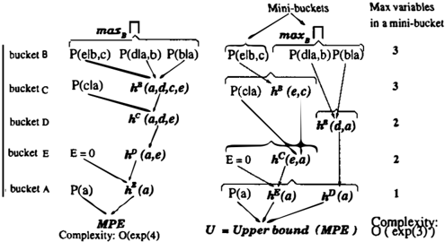
Example 2.3 Figure 3{b) illustrates how algorithms Elim-MPE and Approx-MPE(i) for i = 3 process

Figure 3: Execution of Elim-MPE and Approx-MPE

the network in Figure 1 (a) along the ordering (A, E, D, C, B). Algorithm Elim-MPE records new � unc­ tions hB(a, d,c, e), hc(a, d, e), hD(a, e), and h (a). Then, in the bucket of A, it computes MPE = ma Xa P(a)h E (a). Subsequently, an MPE assignment (A = a', B = b', C = c', D = d', E = 0) { E = 0 is an evidence) is computed for each vari­ able from A to B by selecting a value that maxi­ mizes the product of functions in the corresponding bucket, conditioned on the previously assigned val­ ues. Namely, a' = arg maXa P(a)hE(a), e' = 0, d' = arg max d hc(a', d, e = 0), and so on. The ap­ proximation Approx-MPE ( 3 ) splits bucket B into two mini-buckets each containing no more than 3 variables, and generates hB (e, c) and hB (d, a). An upper bound on the MPE value is computed by max.P(a) ·hE (a)· hD(a). A suboptimal MPE tuple is computed similarly to MP E tuple by assigning a value to each variable that maximizes the product of functions in the corre­ sponding bucket, given the assignments to the previous variables.

3 Heuristic Search with Mini-Bucket

3.1 Notation

In the following discussion we will assume that the mini-bucket algorithm was applied to a belief network using a given variable ordering d = X1, ... , Xn, and that the algorithm outputs an ordered set of aug­ mented buckets bucket 1, . .. ,bucket p, . . . ,bucket n, con­ taining the input functions and the newly generated functions. Relative to such an ordered set of aug­ mented buckets we use the following convention.

• Pp, denotes the input conditional probability ma­ trices placed in bucket p, ( namely, its highest­ ordered variable is Xp).
• h p , denotes an arbitrary function in bucket p gen­ erated by the mini-bucket algorithm.
• h� denotes a function created by the j-th mini­ J bucket in bucket p.
• >. P i denotes an arbitrary function in bucket p.

We denote by buckets(l..p) the union of all functions in the bucket of X1 through the bucket of Xp. Remember that S(f) denotes the set of arguments of function f.

3.2 The Heuristic Function

The idea, first presented in ( Kask and Dechter, 1999a ) , is given here for the completeness of the presentation. We will show that the new functions recorded by the mini-bucket algorithm can be used to express upper bounds on the most probable extension of any partial assignment. Therefore, they can serve as heuristics in an evaluation function which guides a Best-First search or as an upper bounding function for pruning Branch-and-Bound search.

DEFINITION 3.1 (Exact Evaluation Function) Let x = xP = ( x 1, ... , xp)· The probability of the most probable extension of xP, denoted J* (xP) is:

The above product defining f* can be divided into two smaller products expressed by the func­ tions in the ordered augmented buckets. In the first product all the arguments are instanti­ ated, and therefore the maximization operation is applied to the second product only. Denoting g(x) = IlP;E bucketo(l..p)P;(xs(P;)) and H*(x) = max{xp+1, . . . ,X.IX;=x;, V l�i�p} flP;Ebucketo(p+l..n)P;, we.get f*(x) = g(x) . H*(x). During search, the g function can be eva! uated over the partial assignment xP, while H* can be estimated by a heuristic function H defined next.

DEFINITION 3.2 Given an ordered set of augmented buckets, the heuristic function H(xP), is the product of all the h f unctions that satisfy the following two prop­ erties: 1} They are generated in buckets {p + 1, . . . , n), and 2} They reside in buckets 1 through p. Namely, H(xP) = Il f = l IThJEbucket, h J , where k > p, (i.e . h J is generated by a bucket processed before bucket p.)

The following proposition shows how g(xP+1) and H(xP+1) can be updated recursively based on g(xP) and H ( xP) and functions residing in bucket p + 1.

Proposition 1 Given a partial assignment xP = (x 1 , ... xp), both g(xP) and H(xP) can be computed re­ cursively by

THEOREM 3.1 (Mini-Bucket Heuristic) For every partial assignment x = xP = ( x1, .. . , xp), of the first p variables, the evaluation function f(xP) = g(xP) · H(xP) is: 1} Admissible it never underestimates the probability of the best extension of J:P. 2} Monotonic, namely f(xP + 1 ) / f(xP) ::; 1.

Proof. To prove monotonicity we will use the recur­ sive equations (1) and (2) from Proposition 1. For any J;P and any value v in the domain of Xp+1, we have

Since h} +1 (xP) is computed for each mini-bucket j in bucket (p+ 1) by maximizing over variable X P + 1 , ( elim­ inating variable X p + t ) , we get

Thus, f(xP, v) ::; f(xP), concluding the proof of mono­ tonicity.

The proof of admissibility follows from monotonicity. It is well known that if a heuristic function is monotone and if it is exact for a full solution (which is our case, since the heuristic is the constant 1 on a full solution) then it is also admissible [Pearl, 1984]. 0

3.3 Search with Mini-Bucket Heuristics

The tightness of the upper bound generated by mini­ bucket approximation depends on its i-bound param­ eter. Larger values of i generally yield better upper­ bounds, but require more computation. Therefore, both Branch-and-Bound search and Best-First search, if parameterized by i, allow a controllable tradeoff be­ tween preprocessing and search, or between heuristic strength and its overhead.

In Figures 4 and 5 we present algorithms BBMB and BFMB. Both algorithms are initialized by running the mini-bucket approximation algorithm that produces a set of ordered augmented buckets.

Branch and bound with mini-bucket heuristics (BBMB) traverses the search space in a depth-first manner, instantiating variables from first to last.

Algorithm BBMB(i)

Input: A belief network BN = {P 1 , ... ,Pn}; ordering d; time bound t.

Output: An MPE assignment, or a lower bound and an upper-bound on the MPE.

1. Initialize: Run M B ( i ) algorithm which generates a set of ordered augmented buckets and an upper-bound on MPE. Set lower bound L to 0. Set current variable index p to 0.
2. Search: Execute the following procedure until variable X1 has no legal values left, or out of time, in which case output the current best solution.
3. Expand: Given a partial instantiation xP, compute all partial assignments a;P+ 1 = ( xP, v ) for each value v of X v + 1 . For each node a;P+ 1 compute its heuristic value f(.xP+ 1 ) = g(xP+1 ) . H(.xP+1) using

·

g(xP+I)

=

g(xP)

and

H(.xP+1) = H(.xP) . Ihhp +I ./IIih� +1.

lijPp + lj

Prune those assignments a;P+I for which f(.xP+I) is smaller than the lower bound L.

• Forward: If Xp + l has no legal values left, goto Back­ track. Otherwise let a;P+ 1 = ( a;P, v ) be the best extension to a;P according to f. If p + 1 = n, then set L = f(xP+I) and goto Backtrack. Otherwise remove v from the list of legal values. Set p = p + 1 and goto Expand.
• Backtrack: If p = 1, Exit. Otherwise set p = p-1 and repeat the Forward step.

Figure 4: Algorithm BBMB(i)

Throughout the search, the algorithm maintains a lower bound on the probability of the MPE assign­ ment, which corresponds to the probability of the best full variable instantiation found thus far. When the algorithm processes variable Xp, all the variables pre­ ceding Xp in the ordering are already instantiated, so it can compute the heuristic value f(xP-1, Xp = v) = g(xP-1, v) · H(xP, v) for each extension Xp = v. The algorithm prunes all values v whose heuristic estimate (upper bound) f(xP, Xp = v) is less or equal to the current best lower bound, because such a partial as­ signment ( x1, ... Xp-1, v) cannot be extended to an im­ proved full assignment. The algorithm assigns the best value v to variable Xp, and proceeds to variable Xp+1, and when variable Xp has no values left, it backtracks to variable Xp_1· Search terminates when it reaches a time-bound or when the first variable has no values left. In the latter case, the algorithm has found an optimal solution.

Algorithm Best-First with mini-bucket heuristics (BFMB), starts by adding a dummy node xo to the list of open nodes. Each node corresponds to a partial assignment J:P and has an associated heuristic value f(xP). Initially f(x0) = 1. The basic step of the algo­ rithm consists of selecting an assignment xP from the list of open nodes having the highest heuristic value f(xP), expanding it by computing all partial assign­ ments (xP, v) for all values v of Xp+1, and adding them

Algorithm BFMB(i)

Input: A belief network BN = {P1, .·· , Pn}; ordering d; time bound t.

Output: An MPE assignment or just an upper bound and a lower bound (produced by mini-bucket).

1. Initialize: Run MB ( i ) algorithm which generates a set of augmented buckets, an upper-bound and a lower bound assignment. Insert a dummy node x0 in the set L of open nodes. Set f(xo) to 1.
2. Search:
3. If out of time, output mini-bucket assignment.
4. Select and remove a node xP with the largest heuristic value f(xP) from the set of open nodes L.
5. Expand xP by computing all child nodes ( xP, u) for each value v in the domain of X P+ 1· For each node a;P+ 1 com­ pute its heuristic value f(xP+I) = g(xP+I )H(xP+I ) , where g(xP) = g(xP-1). ITjPp1 and H(xP) = H(x p -l) · IIkhp.fiijh�
6. I f n = p then xP is an optimal solution. Exit.
7. Add all nodes ( xP, v ) to L and go to Search.

Figure 5: Algorithm BFMB(i)

to the list of open nodes. The algorithm terminates when it selects a complete assignment for expansion which is guaranteed to be optimal.

4 Experimental Methodology

We tested the performance of our scheme on three types of networks - random coding networks, Noisy­ OR networks and CPCS networks. On each problem we ran both BBMB(i) and BFMB(i) using mini-bucket approximation with various i-bounds. On random cod­ ing networks we also ran for comparison the Iterative Belief Propagation (IBP) [Pearl, 1988], the best algo­ rithm known for probabilistic decoding.

We used the min-degree heuristic for computing the ordering of variables. It places a variable with the smallest degree at the end of the ordering, connects all of its neighbors, removes the variable from the graph and repeats the whole procedure.

We treat all algorithms as approximation algorithms. Algorithms BBMB and BFMB, if allowed to run until completion will solve all problems exactly. However, since we use a time-bound, both algorithms may re­ turn suboptimal solutions, especially for harder and larger instances. BBMB outputs its best solution while BFMB, if interrupted, outputs the mini-bucket solu­ tion. Consequently BFMB is effective only as a com­ plete algorithm.

The main measure of performance we used is the accu­ racy ratio opt= Pa�9/PMPE between the probability of the solution found by the test algorithm ( Patg) and the probability of the optimal solution ( P M p E), given

a fixed time bound, whenever PMPE is available. We also record the running time of each algorithm.

We recorded the distribution of problems with respect to accuracy opt over 5 predefined ranges : opt 2: 0.95, opt 2: 0.5, opt 2: 0.2, opt 2: 0.01 and opt < 0.01. How­ ever, because of space restrictions, we report only the number of problems that fall in the accuracy range opt 2: 0.95. Problems in this range were solved opti­ mally.

In addition, during the execution of both BBMB and BFMB we also stored the current lower bound L at regular time intervals. This allows reporting of accu­ racy as a function of time.

4.1 Random Coding Networks

Our random coding networks fall within the class of linear block codes . They can be represented as four­ layer belief networks (Figure 6). The second and third layers correspond to input information bits and parity check bits respectively. Each parity check bit repre­ sents an XOR function of input bits u;. Input and parity check nodes are binary while the output nodes are real-valued. In our experiments each layer has the same number of nodes because we use code rate of R=K/N=l/2, where K is the number of input bits and N is the number of transmitted bits.

Given a number of input bits K, number of parents P for each XOR bit and channel noise variance o-2, a coding network structure is generated by randomly picking parents for each XOR node. Then we simulate an input signal by assuming a uniform random distri­ bution of information bits, compute the corresponding values of the parity check bits, and generate an assign­ ment to the output nodes by adding Gaussian noise to each information and parity check bit. The decoding algorithm takes as input the coding network and the observed real-valued output assignment and recovers the original input bitvector by computing or approx­ imating an MPE assignment. In our experiments all coding networks were generated by randomly picking

N=lOO K=50 "	MB 88MB BFMB i=2	MB 88MB BFMB i=6	MB BBMB BFMB i=lO	MB 88MB BFMB i-14	IBP
0.22	0.006000 0.000200 0.000200	0.004600 0.000200 0.000200	0.001000 0.000200 0.000200	0.000400 0.000200 0.000200	0.000200
0.28	0.018200 0.001400 0.000200	0.021200 0.000200 0.000200	0.004800 0.000200 0.000200	0.000100 0.000200 0.000200	0.000200
0.32	0.044800 0.007200 0.002200	0.036200 0.002200 0.002200	0.025600 0.002200 0.002200	0.014800 0.002200 0.002200	0.002200
0.40	0.099600 0.019400 0.011600	0.099600 0.012000 0.008800	0.062800 0.008800 0.008800	0.040600 0.008800 0.008800	0.008800
0.51	0.191600 0.098000 0.097400	0.185200 0.083000 0.082200	0.163000 0.076200 0.076600	0.148600 0.076200 0.076200	0.080000

Table 2: Random coding BER, N=100 K=50. 100 samples.

N 100 K= 50 "	opt	8 �� 8 BFMB i=2 #/time	s:;'r::s BFMB i=6 #/time	MB 88MB BFMB i=lO #/time	8 �� 8 BFMB i=14 #Itime	IBP
0.22	>0.95	8�!?·04 100/0.06 100/0.06	89f?·06 100/0.14 100/0.08	9?!?·32 100/0.33 100/0.34	9�!�·26 100/3.26 100/3.27	1o?L 0.09
0.28	>0.95	7��0.04 99/0.38 100/0.13	7?!?·06 100/0.40 100/0.10	8�!?·34 100/0.40 100/0.37	9?!�·13 100/3.14 100/3.39	10�£ 0.09
0.32	>0.95	4:�? OS 96/0.94 100/0.13	S�f?·06 100/0.78 10oio.1o	7 . '!?·34 100/0.40 10oio.37	• . 1!�·34 100/3.39 100i3.39	�.%
0.40	>0.95	'!�?·04 9� � � 13 99 0.87	2��?·06 99/2.20 100/0.64	4Y?·32 100/0.70 100j0.48	6�Ho1 100/3.11 100i3.10	�.%
0.51	>0.95	�!0.04 7� � :2.0 71 9.05	�!�·06 9� � �.15 88 6.84	1�!�·34 1o� p ·s2 99 2.78	18!�·38 10� � � 00 100 4.07	32/ 0.08

I

Table 1: Random coding, N=100 K=50. 100 samples.

4 parents for each XOR bit.

Tables 1 through 4 report on random coding networks. In addition to BBMB and BFMB, we also ran Iterative Belief Propagation ( IBP ) [ Pearl, 1988 ] .

For each u we generated and tested 100 samples di­ vided into 10 different networks each simulated with 10 different input bit vectors 1 We also tried to run Elim-MPE on this set of problems, but the induced width w* was too large and Elim-MPE failed to solve any problems.

In Table 1 there are 5 horizontal blocks, each corre­ sponding to a different value of channel noise u. Each block reports a distribution over the 95% accuracy range. Within each block we have 3 rows, one for each of MB ( mini-bucket ) , BBMB and BFMB. Columns 3 through 6 report the results on various i-bounds. Col­ umn 7 reports results for IBP.

Looking at the third block in Table 1 ( corresponding to u = 0.32 ) , we see that MB with i=2 ( column 3 ) solved 45% of the problems exactly ( opt � 0.95 ) , while tak­ ing 0.05 seconds on the average. On the same set of problems, using mini-bucket heuristics, BBMB solved 96% of the problems exactly while taking 0.94 seconds on the average, while BFMB solved all problems ex­ actly with average time of 0.13 seconds only. When moving to the right to columns 4 through 6 in rows corresponding to u = 0.32 and opt � 0.95 we see the gradual change caused by higher level of mini-bucket heuristic ( higher values of i-bound ) . As expected, MB solves more problems, while using more time. Focus­ ing on BFMB we see that it always solved all problems

'In the past ([ Kask and Dechter, 1999a )) we have run a large number of random coding experiments with differ­ ent variable orderings. The results we report in this paper ( with min-degree ordering ) are typical of all the experi­ ments we have run.

with any i-bound, and its total running time as a func­ tion of i forms a U-shaped curve. At first ( i=2 ) it is high ( 0.13 ) , then as i-bound increases the total time decreases ( when i=6 total time is 0.10 ) , but then as i-bound increases further the total time starts to m­ crease again.

The added amount of search on top of MB can be es­ timated by t,earch = ttotal- tMB· For each value of u, as i increases the average search time t,earch de­ creases, and the overall accuracy of search increases ( more problems fall within higher ranges of opt ) . How­ ever, as i increases, the amount of MB preprocessing increases as well.

Each line in the table demonstrates the tradeoff be­ tween the amount of preprocessing performed by MB and the amount of subsequent search using the heuris­ tic cost function generated by MB. We observe that the total time improves when i increases until a thresh­ old point and then worsens. When i is smaller than this threshold, the heuristic cost function is weak and search takes longer. When i is larger than this thresh­ old, the extra preprocessing is not cost effective.

We observe that as problems become harder ( i.e. u increases ) both search algorithms achieve their best performance for larger i when the mini-bucket heuris­ tics is stronger. For example, in Table 1, when u is 0.22, the optimal performance is for i = 2. When u is 0.40, the optimal point is i = 10.

One crucial difference between BBMB and BFMB is that BBMB is an anytime algorithm - it always out­ puts an assignment, and as time increases, its solution gets better. BFMB on the other hand, is an ali-or­ nothing algorithm. It only outputs a solution when it finds an optimal solution. In our experiments, we always used a time bound. If BFMB did not finish within the time bound, it outputed the MB assign­ ment. From Table 1 we see that when sufficient time

M 4

Table 3: Random coding, N=200 K=100. 100 samples.

N 200 K= 100 q	opt	MB 88MB BFMB i=2 #/time	a ii' i: a BFMB i=6 # I time	MB 88MB BFMB i=lO #/time	MB 88MB BFMB i=l4 #/time	IBP
0.22	>0.95	7;�� 09 98/0.94 100/0.12	8!��.12 98/0.65 100/0.16	9��?·73 99/0.95 100/0.77	9�!�·00 100/8.04 100/8.03	10?! 0.16
0.28	>0.95	4��0 09 84/3.72 100/0.80	4��0.12 88/4.17 100/0.56	5��?·72 96/2.50 100/0.89	1�e·95 99/8.64 100/8.03	10?£ 0.13
0.32	>0.95	1��0.09 63/10.2 94/6.19	. 2!�?·12 68/9.49 96/4.12	3;�o 73 87/6.33 99f2.49	4��8.06 92/10.7 100/8.75	�.��
0.40	>0.95	N/A � � � N A	0/- 28/90.5 39f66.7	. 5J?·n 3� � �18 67 50.1	6J.7.77 5� � :2 7 85 41.1	;��

is given (indicated by cases when both BBMB and BFMB solve all problems) the average running time of BFMB is never worse than BBMB and often better by a factor of 5-10.

In Table 2 we report the Bit Error Rate (BER) for the same problems and algorithms as in Table 1. BER is a standard measure used in the coding literature denoting the fraction of input bits that were decoded incorrectly. We observe that when the noise is very small (0.22, 0.28) BBMB and BFMB are equal to IBP since both BBMB/BFMB and IBP solve all problems exactly. However, when noise increases (0.51) BBMB and BFMB outperform IBP when the i-bound is suf­ ficiently large. We ran 30 iterations of IBP on each problem and noticed that usually it converged to the final assignment after 5-10 iterations. Giving it more time would not improve its performance.

This phenomenon is more pronounced in Tables 3 and 4, where we present results with K=100 input bits. In this set of experiments we increased the time bound from 30 sec to 60 seconds (for small noise) or to 180 sec­ onds (for large noise), while doubling the problem size. Again, we see a similar pattern of preprocessing-search tradeoff as with networks of K=50 bits. Also, we ob­ serve the superiority of BFMB over BBMB. Given the same i-bound, BFMB can solve more problems than BBMB and faster.

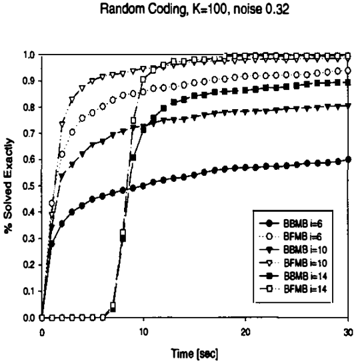
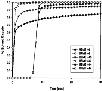
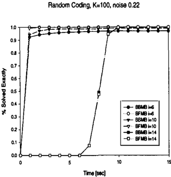
In Figures 7, 8 and 9 we provide an alternative view of the performance of BBMB(i) and BFMB(i). Let FBBMB(i)(t) (FBFMB(i)(t)) be the fraction of the problems solved completely by BBMB(i) (BFMB(i)) by time t. Each graph in Figures 7, 8 and 9 plots FBBMB(i)(t) and FBFMB(i)(t) for some specific value of i.

Figures 7, 8 and 9 display a trade-off between pre­ processing and search. Clearly, if FBBM B(i) (t) > FBBM B(i) (t), then FBBM B(i) (t) completely dominates FBBMB(i)(t). For example, in Figure 9 BBMB(10)

Table 4: Random coding BER, N=200 K=100. 100 samples.

N=200 K=IOO q	MB 88MB BFMB i=B	MB 88MB BFMB i=lO	MB 88MB BFMB i=l2	MB 88MB BFMB i=l4	IBP
0.22	0.004280 0.000680 0.000220	0.003780 0.000600 0.000220	0.002100 0.000340 0.000220	0.001200 0.000220 0.000220	0.000220
0.28	0.020260 0.007820 0.001020	0.020580 0.006040 0.001020	0.015320 0.002620 0.001020	0.009220 0.001360 0.001020	0.001040
0.32	0.042840 0.023780 0.006660	0.043740 0.021340 0.006060	0.038060 0.010980 0.003520	0.027600 0.007280 0.002820	0.002820
0.40	��A N/A NfA	0.115200 0.083500 0.081200	0.105100 0.054900 0.050900	0.097300 0.047400 0.026400	0.011700

15

completely dominates BBMB(6). When FBBMB(i)(t) and FBBM B(i) (t) intersect, they display a trade-off as a function of time. For example, if we have only few seconds, BBMB(6) is better than BBMB(14). How­ ever, when sufficient time is allowed, BBMB(14) is su­ perior to BBMB(6).

Figures 7, 8 and 9 also show that FBFMB(i)(t) always dominates FBBM B(i) (t) for any value of i.

4.2 Random Noisy-OR Networks

Random Noisy-OR networks were randomly generated using parameters (N, K, C, P), where N is the number of variables, K is their domain size, C is the number of conditional probability matrices and P is the number of parents in each conditional probability matrix.

The structure of each test problem is created by ran­ domly picking C variables out of N and for each, randomly selecting P parents from preceding vari-

Random Coding, K=100, noise 0.28

Table 5: Noisy-OR MPE. Pnoise=0.2, Pleak=O.Ol. 10 evidence variables.

N c p	opt	MB 88MB BFMB i=2 #f time	8 ;;'� 8 BFMB i=6 #I time	MB BBMB BFMB i = lO #/time	MB BBMB BFMB i=14 # - �time
128 85 4	>0.95	10��0.05 100/0.95 100/!.76	10��0.08 100/0.59 100/l.l9	10��0.65 100/0.98 100/!.37	10��8.07 100/8.47 100/8.56
128 95 4	>0.95	9�!� 06 10� ? 68 100 2.68	9�f� 09 10� � : [.68 100 2.58	9�!�·7 4 10� ? 69 100 2.47	9�!�·06 10� � �·70 100 9.96
128 105 4	>0.95	99J?·08 10� ? 72 100 4.83	·�!�·10 10� ? 24 100 4.37	·�!?·80 10� ? ·80 100 2.87	••! . 10.0 10� � 10 9 100 11.7

abies, relative to some ordering. Each probability ta­ ble represents an OR-function with a given noise and leak probabilities : P(X = 0\Yt, ... , Yp) = P1eak X llY;=lPnoi&e·

Table 5 presents results of experiments with random Noisy-OR networks. Parameters N, K and P are fixed, while C, controlling network's sparseness, is changing.

Here we see a similar pattern of tradeoff between mini­ bucket preprocessing and search. Mini-bucket algo­ rithm can solve most of the problems exactly, but it takes a considerable amount of BBMB/BFMB search time to actually prove the optimality of the mini­ bucket solution. We also see that here Branch and Bound is slightly faster than Best-First. This is be­ cause the lower bound used by BBMB is optimal from the beginning (MB solves the problem), the heuristic function is accurate (! = r) and there are many solu­ tions. However, Best-First expands many more nodes before finding a solution because we use a random tie­ breaking rule.

Table 6: CPCS networks. Time 30 and 45 resp.

CPCS360b 100 samples 10 evid.	MB BBMB BFMB i -4	MB BBMB BFMB i -8	MB BBMB BFMB i-12	MB BBMB BFMB i -16
>0.95	·�1?·9. 1 1. 100[0.93) 10oio.98j	93 1?· 9 �! . 100[0.9: ! 100j0.96	·� 1� 9� 1. 10� [ �·00) 100 2.ooi	9� 1 �5 . 8 ! , 100[15.: ! 10oj15.8
CPCS422b 100 sa.mples 10 evid.	MB BBMB BFMB i=4	MB BBMB BFMB i=B	MB BBMB BFMB i=l2	a:�a BFMB i=16
>0.95	4���2 �! · � [ r : � 97 25.9	4 �� �3. �! 98[24.5) 97[24.5i	5 :1 �2. 11, 100[22.9) 10oi2a.ii	5� J�··o 1. 100[39.0) 10oia9.1i

4.3 CPCS Networks

As another realistic domain, we used the CPCS networks derived from the Computer-Based Patient Care Simulation system, and based on INTERNIST­ I and Quick Medical Reference expert systems [Pradhan et al., 1994]. The nodes in CPCS networks correspond to diseases and findings. Representing it as a belief network requires some simplifying assump­ tions, 1) conditional independence of findings given diseases, 2) noisy-OR dependencies between diseases and findings, and 3) marginal independencies of dis­ eases. For details see [Pradhan et al., 1994].

In Table 5 we have results of experiments with two binary CPCS networks, cpcs360b (N = 360, C = 335) and cpcs422b (N = 422, C = 348), with 100 instances in both cases. Each instance had 10 evidence nodes picked randomly.

Our results show a similar pattern of tradeoff between MB preprocessing and BBMB/BFMB search. Since cpcs360b network is solved quite effectively by the ap-

proximation scheme MB, we get very good heuristics and therefore, the added search time is relatively small, serving primarily to prove the optimality of MB solu­ tion. On the other hand, on cpcs422b MB can solve less than half of the instances accurately when i is small, and more as i increases. BBMB/BFMB are roughly the same, both enhance MB's solution qual­ ity, significantly. They. can solve all instances accu­ rately for i 2: 12. For comparison, elim-mpe solved the cpcs360 network (with no evidence) in 115 sec while for cpcs422 it took 1697 sec. Processing the networks with evidence is a much more challenging task, how­ ever.

5 Discussion and Conclusion

Our experiments demonstrate the potential of mini­ bucket heuristics in improving general search. The mini-bucket heuristic's accuracy can be controlled to yield an optimal tradeoff between preprocessing and search. We demonstrated this property in the context of both Branch-and-Bound [Kask and Dechter, 1999a] and Best-First search. Although the best threshold point cannot be predicted apriori a preliminary em­ pirical analysis can be informative when given a class of problems that is not too heterogeneous.

The mini-bucket heuristics can facilitate Best-First search on relatively sizable problems, thus extending the boundaries of this search scheme which is compu­ tation optimal (relative to search algorithms having access to the same heuristic) for achieving exact solu­ tion. Indeed, we showed that Best-First usually out­ performs Branch-and-Bound, sometimes by a factor of 5-10.

We showed that search can be competitive with the best known approximation algorithms for probabilis­ tic decoding such as IBP when the networks are rel­ atively small, in which case search solved the prob­ lems optimally. Obviously when problem sizes increase BBMB and BFMB require much more time. However, as much as IBP is efficient, its performance will not improve with time.

Finally, since mini-bucket elimination is applicable across many problem tasks such as probabilistic in­ ference and decision making the scheme proposed here has potential of being widely applicable.

References

[Bertele and Brioschi, 1972] U. Bertele and F. Brioschi. Nonserial Dynamic Programming. Academic Press, 1972.

[Dechter and Pearl, 1985] R. Dechter and J. Pearl. Generalized best-first search strategies and the op­ timality of a*. Journal of the ACM, 32:506-536, 1985.

[Dechter and Rish, 1997] R. Dechter and I. Rish. A scheme for approximating probabilistic inference. In Proceedings of Uncertainty in Artificial Intelligence {UAI97), pages 132-141, 1997.

[Dechter, 1992] R. Dechter. Constraint networks. En­ cyclopedia of Artificial Intelligence, pages 276-285, 1992.

[Dechter, 1996] R. Dechter. Bucket elimination: A unifying framework for probabilistic inference al­ gorithms. In Uncertainty in Artificial Intelligence {UAI-96), pages 211-219, 1996.

[Kask and Dechter, 1999a] K. Kask and R. Dechter. Branch and bound with mini-bucket heuristics. Proc. IJCAI, 1999.

[Kask and Dechter, 1999b] K. Kask and R. Dechter. Stochastic local search for bayesian networks. In Workshop on AI and Statistics {AISTAT99}, 1999.

[Pearl, 1984] J. Pearl. Heuristics: Intelligent search strategies. In Addison- Wesley, 1984.

[Pearl, 1988] J. Pearl. Probabilistic Reasoning in In­ telligent Systems. Morgan Kaufmann, 1988.

[Peng and Reggia, 1989] Y. Peng and J.A. Reggia. A connectionist model for diagnostic problem solving. IEEE Transactions on Systems, Man and Cybernet­ ics, 1989.

[Pradhan et al., 1994] M. Pradhan, G. Provan, B. Middleton, and M. Henrion. Knowledge engineer­ ing for large belief networks. In Proc. Tenth Conf. on Uncertainty in Artificial Intelligence, 1994.

[Rish et al., 1998] I. Rish, K. Kask, and R. Dechter. Approximation algorithms for probabilistic decod­ ing. In Uncertainty in Artificial Intelligence (UAI98}, 1998.

[Santos, 1991] E. Santos. On the generation of alter­ native explanations with implications for belief revi­ sion. In Uncertainty in Artificial Intelligence {UAI91), pages 339-347, 1991.

[Shimony and Charniak, 1991] S.E.

Shimony and E. Charniak. A new algorithm for finding map assignments to belief networks. In P. Bonissone, M. Henrion, L. Kanal, and J. Lemmer Eds. Uncertainty in Artificial Intelligence, volume 6, pages 185-193, 1991.