Modeling Uncertain Temporal Evolutions in Model-Based Diagnosis

Luigi Portinale

Dipartimento d i Informatica- Universita' di Torino C.so Svizzera 18.510149 T o r i n o (Italy)

Abstract

Alt h o ugh the notion of diag n ost ic pr o b ­ lem has been extensively i n v e s t i g a t e d in the c o n te x t of static systems, in most p ra c ti c al appli c a t i o n s the behavior of the m o dele d system is s i gn i fican t l y variable d u r i n g time. The g oa l of the paper is to propose a nmel approach to the modeling of uncertainty about temporal evolutions of time-varying systems a n d a charact.er­ ization of m o d el -based temporal d i a g n o ­ sis. Since in most real world cases knowl­ edge about the temporal evolu ti o n of the system to be d iagn o s ed is uncertain, we consider the case when probabilistic tem­ poral knowledge is available for each com­ ponent of the system and we c h oo s e to model it by means of Markov chains. In fact, we aim at exp l o i t i n g the statistical assumptions underlying reliability theory in the context o f the diagnosis of t i me ­ varying systems. lVe finally show how to exploit 1\Iarkov chain theory in order to discard, in the di a g n o s t i c process, very u n l i k e l y d iag n o s e s .

1 INTRODUCTION

The n o t i o n of diagnostic r e as o n in g , and in p a r t i c u ­ lar of model-hased diagnosis, has been extensively investigated i n the past and two bas i c p a r a d i g ms emerged: the logic and the probabilistic one. In the logic p a r ad ig m it is often the case that the m o d e l represents the f u n c t i o n and structure of a device; in this case th e model usually r e p re s e n t s the normal b e hav io r of a system and the d i a g n o sti c reasoning follows a consistency-based approach [ 21 ] (the diagnosis is a set of abnormality a s s um p t i o n s on the components of t h e system that, together with the observations, r e st or e the consistency in the model). Alternatively, t he use of causal mod­ els has been proposed to model the f a u l ty behavior of t h e system where an abductive approach is used [19] (the di a g n os i s must cover the observations). !3oth a ppro a c h e s use a logical model of the sys­ tem to be diagnosed and it has been shown that they are just the extremes of a spectrum of logical definitions of di a gn o s is f6). On the other hanJ, in the probabilistic paradigm, diagnostic kuowleJge is usually represent.ed by means of associations be­ tween symptoms and disorders; per f o r m i n g a J.iag­ nosis means finding the most probable set of dis­ orders, g i v e n the s y m pt o m s . The major part of the work in probabilistic dia g no s i s has been con ­ cerned with the use of Bayesian methods baseJ. on belief networks [17] as in IVIUNIN [1], in Q!IIR-BI\" [22] a n d in [12]. However, other approaches have been p r o p os e d , for instance, r e l y ing on Dempster­ S h a f er theory [13] or on the i nte g r a t i o n of B a y es i a n classification with the set covering moJel [18].

These two basic p a ra di gms to dia gn o s i s seem to be c o m p l em e n t a r y for certain aspects (for example, probabilistic d i a g n os t i c reasoning well a<.hlrcsses t he problem of minimizing the c o s t of I he com­ putation, wh i l e l o gi c -b a s ed reasoning is in g e n e r a l more flexible in dealing with mu l t i p l e disorders or contextual information); for this reason some <It­ t e m p t s have been made for combining them. In fact, probabilistic i n f or m a t i o n has been integrated in logical d i a g n o s ti c framework either for defin­ ing criteria for choosing the best next. measure­ ment [5,8] or for extending probabilistic diagnostic f r a mew o rk s to non propositional fo r m [20]. How­ ever, the c o n t e x t in which s u c h approac!Jes ha,·e been proposed i s m a inl y that of static system> in which the system behavior can be thought a:> fixed during the d i a g n ost ic process and s o time indepen­ dent. C l e a r ly , in i mp orta n t applications this is not sufficient, because the modeled system is int.rinsi-

cally d y n a mi c and its behavior i s s i g n i fic a nt l y v a r i ­ a b l e d u r i n g time. For t h i s reason there is a grow­ ing inte r e s t in the s t u d y of t h e behavior of time­ va r yin g systems in the attempt of e i t h e r extend­ ing st a t i c diagnostic techniques [14] or fi n d i n g new ap p r o a c he s more suitable for time-dependent be­ h a v i o r [11). Diagnosing systems with time-varying behavior r e q u i r e s the ability of d e a l in g at least with the f o l l ow i ng i m p o r t a n t a s p e c t s : o b s e r v a t i o n s a c r o s s d iff e r e n t t i m e i n s t an t s a n d e x p li c i t d e s c rip ­ tion of state changes of the system w i t h r e s p e c t to time. One of the immediate consequences of the s e aspects of the p ro b l e m is t he need of having some form of abstraction in the model r ep r e s e n t i n g the system to be d i a g n o sed ; in fact, a l t h o u g h some of the earlier ap p r o a c h e s to diagnosis of dynamic sys­ t e m s tried to deal w i th s in g l e level description of the system [24), most of the recent pr o p o s a l s are f o c us e d on the possibility of having a hi e ra r c h i c a l model in w h i ch multiple l a y e r s of a b s t r a c t i o n s can be used in order to perform t h e diagnostic task [14,1G].

In pr e vi o u s works we concentrated on a b d u c t i v e r e a !; o n i n g as an useful f r a m ew o r k f o r d i a g n os i n g static systems, even if s o m e attention has to be paid for m i t i gat i n g t.he c om p u t a t i o n a l c o m p l e x i t y of the a b d uc ti ve process [2]. However, e x t e n d i n g tlwse mechanisms in the d i r e ct i o n of time-varying s y s t e m s can lead to sev e r al problems. F i r s t of all, in m o s t real world cases temporal i n f o rm a t i o n is un c e r t ai n and not a l \ \ " ay s easy to encode in the model of the system to be d ia g n o se d . The use of propagation techniques for fuzzy temporal inter­ vals has been proposed in[4] a n d [ l O ] , but even if in practice we can determine the t e m po r a l evolutions o f the system in a m o 1 · e precise way, serious p r o b ­ lems arise from the computational p o in t of v i e w [I]: t h i s means that s o m e kind of approximation has to be considered.

In particular, we are i n te r es t ed in analyzing h o w to exp l o i t , i n a. component-oriented m o d e l , p r o ba ­ b il i sti c k n o w l e d g e about p o s s i b l e t e m por a l evolu­ tions of the component.->. In particular we assume that.:

• components have a d i s c r e t e set of diff e r e n t be­ h a t'tOT'al modts [D] (a b e h a v i o r a l mode repre­ sents a p a rt i c ula r state of a component; t h e set. of behavioral modes consists of o n e "correct" mode a n d , in general, several a b n o rm a l m o de s representing fault.y c o n d iti o n s of the compo­ nent).
• f:'ach component c a n c h a n g e i t s m o d e d ur in g time. w h i l e the manifestations of a behavioral mode are inst.<1nt.aneous (with r e s pec t to the
• amount of time required for a t r a n s i t i o n be­ tween two behavioral modes, or the amount of time e l a p s i n g between two consecutive time points with observations ) ;
• k n o w l e d g e about the temporal e vo l uti o n of a component is uncertain and has to he modeled at some level of abstraction.

The a i m of t h e paper is to propose, given this kind of a ss u mp t i o n s , a. characterization of tempo­ r a l d i a g n os i s in s u c h a way that di a g n o s t i c tech­ niques, developed f o r static systems, could be used a s much as p o s s i b le in the d i a g n o s i s of systems ex­ h i b i t i ng t i m e -va r yi n g behavior. This is pursuE;d h av i ng in mind the fact that t e m p o ral information is abstracted from o t h e r behavioral features of the sy s t e m , s u c h as the r e l a t i o ns h i p s bel\Yeen beh a v ­ ioral modes of the c o m p o n e n ts and their observable manifestations; t h i s means that such relationships do not t a k e into account t im e which is a d de d 1.0 the model as an o r t ho g o n a l dimension ( see also [15]). The kind of ab s tract io n we use throughout the pa­ per is a pr o b a b i l i s t i c one. We assume to have at d i s p o s a l probabilistic knowledge a b o u t the tempo­ ral behavior of the components of the system to be diagnosed in s u ch a way that such behavior ca.n be m o d e le d as a st o c h a s t i c process; in particular, we aim at ex p loiting t h e theory of markovian stochas­ tic processes in a di a gn o s t i c setting by adopling the usual assumptions followed in reliability theory [23]. In fact, t h i s k i n d o f pr o ba b i l i s t i c know ledge can be su p p o s ed to be available from t h e statistics about the b e ha vi o r of the system. We will s h o w h o w th i s a p p r o a c h can be used in orJer to dis­ c a r d t e m por a l evolutious which are v e r y unlikely, however, for the lack of s p a c e , we discussed here just the declarative characterization of the prob­ lem, without co n s id e r i ng r e as o n i n g issues.

2 STOCHASTIC PROCESSES AND RELIABILITY THEORY

In t h i s section, we briefly recall some basic n o t i o n s relative to stochastic processes and the proba bi l i s ­ tic a s s u m pt i o n s usually a do p t e d in r e l i a bi l ity the­ o r y , concerning the life cycle of a c o mp o ne n t of a p h ys i c a l s y s t em .

Definition 1 A stochastic process is a ja111ily of random variables {X(t)jt E T} defined Ot'U lhe same probability space, taking values in a stl Sand indexed by a pam meter t E T.

The values assumed by the v a r i a b le s of the s t oc h a s­ tic process are ca ll e d states and the setS is called the stale space of th e process. Usually the p;name-

t.er t re pr e s e n t s time, so a stochastic process can be thought as the model of the evolution of a system across time1. In t h e following we will concentrate on chains (i.e. discrete-state processes ) wi th dis­ crete time pa r a m e t e r and in par ti c ula r on Markov chains.

Definition 2 A Markov chain is a discrete­ state stochastic process {X(t)/t E T} such that for any to < t1 < . . . t11 the conditional distribution of X(tn) for given values X(to) . .. X(tn-d depends only on X(t11_t) that is:

We will be concerned only with Discrete-Time l\Iarkov Chains (DTl\IC). In a 1\Iarkov ch a i n , the p ro b abil i t y of transition from one state to another depends only from t h e current state and from the current time ins ta n t . If the c on d i t i o n a l probabil­ ity showed in the above definition is i n v a ri a nt with respect to th e time o r ig i n , then we have a so called time -hom:ogeneorts Markov chain; this means t h a t

In this case, the past h i s t o r y of the chain is com­ p l e t e ly summarized in the current state; with the assumption of time-homogeneity, it can be shown t ha t , in the case of a DTMC, the sojoum time in a given state follows a geometric distribution. T h i s is the only distribution satisfying the memo­ ryless property, for a discrete r a n d o m variable (the corresponding m e m o r yl e ss distribution for a. con­ tinuous variable is the exponential distribution). A d i sc r e t e random variable X is geometrically dis­ tr i b u t e d with p a r a me te r p if its probability mass function is pmf(l) = P(X = t) = p(lp ) 11· We say that X has the memory less property if a n d only if P(X = t + niX > t) = P(X = n); t hi s means that we need not remember how l o n g the process has b e e n spending time in a given state to d e t e r mine the probabilities of the n e xt possi­ ble transitions (i.e. we can a rb i tr ar il y choose the o r i gi n of th e time axis ) . In the following we will consider only timc-lwmogeneous DT�IC.

Reliability theory copes with the application of particular probability distributions to the analysis of the life cycle of t.he components of a. physical sys­ tem. In particular, it. has been recognized that the life of a c om p o n e n t can be subdivided into three

1 In t.he following we will refer t.o t as t.he t.ime pa ra.met er.

phases: the infant mortality phase where the fail­ ure probability pis d e c r easi n g with time, the us11al life p h a s e with constant failure probability anll the wear-out phase w h er e the f a i l u r e probability is in­ creasing with age. If we consider the lifetime X of a co mpo n e n t to be a d i sc r e te random variable:?, in t h e usual life phase X follows a geometric di�tri­ bution with paramet.er p.

3 DIAGNOSTIC FRAMEWORK

In the i n t ro d u c t i o n , we discussed problems con­ cerning the management of temporal information in di a g n os t i c systems; one of t h e basic difficulty is relative t o t h e a pp r o a c h to be followed in model­ i n g such a k i n d of information. Since a lot of \\'ork in reliability theory has lead to well defined stat i s ­ tical a s s u m p ti o n s about the temporal belJavior of t.he components of a system, we aims at extend­ ing such assumptions in a model based diagno_,;tic framework.

3.1 REPRESENTATIONAL ISSUES

Following the approach proposed i n [3], we choose to decompose the model of the sys t e m to be diag­ n o s e d into two parts:

• a logical static behavioral model ( w i t h no representation of ti m e);
• a mode transition model showing the pos­ sible t e mpo r a l evolutions of the behaYioral modes of e a c h component of t h e system.

However, differently from [3], \\'e c on c e n t r a te here on a d i ff e r e n t characterization of the mode tran­ s i tion model concerning uncertain temporal i n f o r ­ mation. 'Ve assume time to be discrete, allCl use n a t ural numbers to denote time p o in ts . �lore im­ po r ta n tl y , we extend the basic a s s u mp t i on con­ ceming the p r ob a b i l i t y distribution of lite liklime of a com p o n e n t in th e usual life phase to the dif­ ferent b e h avio r a l modes of the compoucnt. Tl1is means that we assume a memoryless Jistribution of the time s pen t by a component in a giveu ll!ude, so the state transition model will be a J)'L\IC. Let. us d i s c u ss in more detail the represe11tationa.l is­ s u e s; we assume that each component of the sys­ t e m has a set of p o ss i b l e behavioral m o de s , (one of which is the "conect" mode). The modes of a c o m p o n e nt are mutually exclusive with respect to a g i ve n time point. The fact that a c o mpo n e 11 t . c is in

2It. is possible to generalize to the coutinuous case (exponential lifetime) by considering the foilure role instead of t.l1e failure probability.

behavioral modem at t im e l i;; l"l'lll'l'>'l'lll<'d hy l lw atom m(c, t). The relationships betll'<'<'ll lwliav­ ioral modes and t he i r manifestations a r e c-xpr<'S:'<'d as Horn c l a u s e s and the model is at e m p o r a l (src [3] for more details). Temporal information is ab­ s t r a c t e d from the logical m o d e l and is r e p r e s e n t ed in a st o c h a s t i c way. Let C O AI P S be the set of components of t.he system to be diagnosed.

Definition 3 Tlte Associated Markov Chain AMC(c) of a component c E COM PSis a llfarkov chain 1those states represent behavioral modes ofc.

It is c l e a r that, assuming time to be d i s c r et e each A .. M C will b e a DT�IC. Furthermore, if p; is t h e probability of being i n the current mode m; at the next t i m e instant, then the sojourn t i m e 5; i n m; is geometrically distributed with parameter ( 1 -p;) i.e. P(Si = t) = p;- 1 (1p;). N o ti c e that, assum­ iug that. a component has several fault modes and modeling the t ru n s i t i o n s among s u c h modes as a �[arkov chain allows us to g e n e r a l i ze the c o n c e p t of fail me probability to the concept of t r ansiti o n probability f r o m one mode to anot.her.

Definition 4 Ltt AMC(c) be tf1e Associated Marko1: Chain of a component c E COM PS rwd p,,,,1(c) be the transition probability from m o de m; t o mode mj of the component c; the matnr Pc = [Pm,m;(c)] i� called the transition proba­ bility matrix of the elwin.

The matrix Pc r ep r ese n t s the transition p ro ba b i l i ­ tiP.s f r o m one mock to a n o t h e r in onP. time im;tant. The probabilistic b e h a v i o r of a M a r k o v chain is completely determinct..! by its transition probability mat.rix and the iui t.i<�l p r o b a b i l i t y distribution. In fact, let iTc(n) = {p;;,,(c),p�,�(c), . . . }he the vector representing the probabilities of the states ( m o d es ) of the chain A.MC( c) at the i n s t a n t 11 (p�,, (c) is the probability of the c o m p o n e n t c b e i n g in m o d e . n�; at t i m e n); th i s distribution depends on the mJ­ tial distribution of modes, i nd e e d the fundamen­ tal r e l a t. i o n among mo d e probability clist.ribut.ion is given by

\Yhere the (nth power) m a tr i x P e n = [p:;,.,m/c)J and p;;, ., (c) is the probability of reaching m o d e Ill· fro1;1 ! � 10cle m; in n time instants of t h e com­ p�nent c. �1oreO\'Cr, an interesting characteristic of \linkov chains is t h e possibility of classifying its states in a rigorous way.

• an ugodic sd of st.at.es is a set. in "·hich every state can be reached f r o m every other state am! which cannot be left once entered; eaclJ t:·lE"ment of the set is called ergodic ,�tate:
• a lnnt.�inll sd of states is a se t in which C\·cry sl.at.f' can be reached from e ver y other state and which can be left ; each element of the set is called transient state;
• an a b s o r b i n g state is a state w h i c h once en­ tered is never left ( i . e . the probability of re­ maining in t.his state once enteret..! is 1);

An in te r e s t i n g way of exploiting this cla�>sification is to use the AMC(c) to g i v e an a-priori c l ass i fi ­ cation of faults3. Given the AMC(c), let m; be a f a u l t m o d e o f c:

• m; is a permanent fault iff it corresponds to an absorbing state of AMC(c);
• m; is a transient fault iff it corresponds to a t r a n s i e n t. state of A.MC(c);
• m; is a ret·ersible fault iff p;�.mo (c) > 0 for some n and m0 is t h e correct mode;
• m; is an irrevers _ ible fault iff p�,,�(c) = 0 for e v e r y 11 and m0 IS the correct mode.

3.2 CHARACTERIZATION OF A TEMPORAL DIAGNOSTIC PROBLEM

In order to show how stochastic infonnatioll can be i nte g ra t e d in a logical model based diagnos­ t i c framework, in this s e c t i on we briefly di:-;cuss a possible characte-rization of a temp o r a l di<�giiOS­ tic p r o bl em. \\'e can d e f m e a temporal dtagnosltc problem TPD as composed by a b e h a Y io r a l model B M, a s e t of components COM P S and a set of observat.ions at. different t i m e instants OBS to l>,; explained\ we can extract from a TPD a corre­ sponding atemporal diagu ostic problt m APD by c o nsi d e r i n g a set of o b s e r v a t i o ns 0 BS(l) at a gi V\:11 time i n s t a n t t. Solving an atemporal dia g nvstic problem at the instant t means t o clet ermine an assignment at timet, !V(t), to each componem i n COM PS explaining the observations in OIJS(t). This as s ig nm e n t is an atemporal diagnosis. Ob­ viouslv the time instants which are of interest in the d i � � n o s t i c process are just those for whid1 we have some observations; we w i l l call such inst<mts rdtvant time insta11ts. Let us assuu1e, as iu the most part of the previous work on diagnosis, t !I at each c o m po n e n t is independent of e at h other (i.e.

J A similar proposal is presented in [11] hy introduc­ ing an O·Jloslerior·i classilica.tion.

4 The suitable notion of explanation can !Je t:X­ traded from the �pectrum of definitions ill [G]; more­ oYer, notice that, for the sake of simplicity, we tlo nol discuss the role of contextual informat.ioH in a diagllos­ tic problem (see [G] for an analysis of this pro hlc·lll ) .

t.he b e ha v i o r of a component c a n n o t influence the behavior of the others). \'Ve indicate as mtv(!) the m o d e that W(t) assigns to c; because of the in­ dependence of the co m p o n e n t s 1 if ti < t j are two relevant time instant, we have

and c l e a r ly

,,·here p�1c (c) d�pends on the initial distribuw(t) t.ions iTc(O) gi v e n for each component c. More­ over, we a r e also interested in the joint probability P[W(O), W(l), . . . W(t)] at time t of a wh o l e evolution {W(O) . .. Tl'(t)}. Since the analysis of the prob3bilities at time t requires knowledge a b o u t the initial distribution of modes, i n the absence of specific information we can reasonably assume an uniform distributio11.

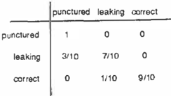
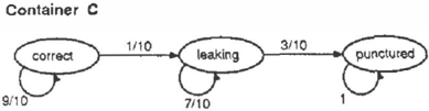
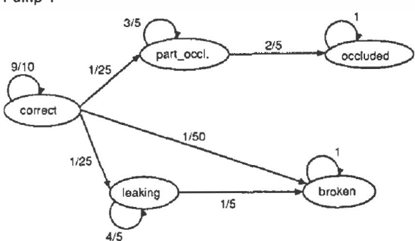
Example 1: l e t us su p p o s e to have a simple sys­ tem composed of a water pump P and a container C receiving the pumped \\·ater. For the sake of b r e v i t y we do not describe the l o gi c a l behavioral model of this simple system, so we will suppose to have directly at d isp os a l the atemporal d i a gn o s e s at the relevant instants. The Ar.ICs of the two components and the transition probability matri­ ces are s ho w n respectively in figure 1 and in figure :2. S u p p o s e to have the following hypothesis at t . i m e t = 0:

Dy a s s u mi n g an uniform distribution we get P[TFdO)] = P[TF:!{O)] = P[W3(0)] = � This means that we have t h e f o l l o w i ng initial distribu� tion on t.he c o m p o u c n t s ( we assume the probabil� ities given in the following o r d e r : pun ct-und, {tak� ing. correct for C and broken, occluded, leaki11g, Jlartially_occlucld, correct for P).

Let. us introduce t.he f o ll o w i n g abbreviations we 11· i l l use in the examples: punctured=zm, !eak­ irl g = le . correct=co. b r o k e n = b r , occluded=oc, par­ twlliJ-OCcluded=po. S u p p o s e that <�t ti m e t = 1 the logical model concludes the atemporal diag­ nosis rr( 1) = {ocdttded(P), coJTect(C)}, then we ha1·e the f o ll o w i n g conditional probabilities

4/5

and the f o llo w i n g joint proba bilit.ies

It is now possible to define a notion of temporal diagnosis on the basis of the c o n c e p t of soluLion for an a t e m p o r al problem.

Definition 5 Given an atemporal diagno�lic pr o blem APD, an assignment W(t) of beharioral modes to e a c h c E COM P S is a temporal di­ agnosis for the corresponding temporal diagnostic problem iff:

1. W(t) is a solution for ADP for evuy n:.leuud time instant t;
2. for et,ery consecutive relevant tir!le iils/a,tb t; < ti, P[W(t1)\W(t;)]2': fJ wheH 0 :S <J :S 1 is a predefin ite threshold named the plausi­ bility threshold for· the temporal diagnostic problem.

Notice t ha t the s e c o n d part of the deftJJit ion c o u ld be different if we s u p p os ed to h a v e inform<ttion on t h e plausibility threshold d ir e c t l y on the com-

，

Pp : transition probability matrix for component P

	i>rol<.en	occ\udeo	\eal<.ing	pan_occ\.	coneCI
broken		0	0	0	0
occluded	0		0	0	0
leaking	liS	0	415	0	0
part_occl.	0	215	0	315	0
correct	1150	0	1/25	1/25	9110

F i gu r e 2: Transition p r o b a b i l i t y matrices of the components P and C

ponents; in this c a s e we c o u l d check the p l a u ­ sibility of the transitions of each component c from ; . = m�V(t,) t.o s = m�Y(tiJ" Obviously, in this c a s e the corresponding t h r e s h o l d should be different; indeed, giv e n the same threshold CT, i f P[IV(tj ) I W(t; )] � u and n = tj l ; , t h e n P�s � u but not vice versa.

The information in t. h e lVI arkov c h a i n s associated with the components can t h e n be used to d i sc a r d very i m p r o b a bl e d i a g n o s t i c hypotheses from the t e m p o r al point of view.

Example 2: g i v C' n t. h e same system of exam­ ple 1, s u p p os e m� g e t the atemporal diagnosis T T ' ( O) = {con·eci (P, 0) , correct(C, 0)}. C o ns i d er now the case in which new observations allow us t.o c o n c l u d e , at time t = 1 the following diagnostic hyp o th e s e s :

Let t he plausibility threshold be u = 1�0 .

The only a d mi ssi b l e diagnosis at time t = 1 i � l r-:> ( 1 ) . By co m p ut i n g the s q u a re matrices PpJ

and PC 2, i t i s easy t o see t h a t. , i f the same di a g ­ noses were concluded at time t = 2, t h e n t.he only non-admissib1e diagnosis would he the fm;t one.

It should be clear that an interesting aspect of t hi s approach is the p o ssi b i l ity of ranking tl1e temporal di a g n o s e s we get; indeed, it is easy to show that the j o i n t probabilities at time t can be recursi,·cly com p u t e d , g i v e n the a-priori distributions P[IF(O)] by the following formula:

where the first factor is the joint probability at t h e previous step and the second can be computed by m e a ns of the ma t r i c e s P c k . For i n s t a n c e , i n ex a m p l e 1, the most probable te m p o ra l diagnosis is { W3(0) , W(l ) } .

4 DISCUSSION

In t h i s paper, an approach i ntegrating stoclws­ tic i n f or m a t i o n i n logical model-based diagnosis is proposed, i n the attempt to characterize proJ,Iems deriving from the i n t r o d u c ti o n of t em p o ral infor­ m a t i o n in the model of the system to be diagnosed. However, an important problem s t i l l to be consid­ ered c o ncer n s the role of t h e AMCs of the compo­ nents with r e sp ect to the u n d er l y i n g static logical model. In fact, using the approach described in t h i s paper, we assume to mo d e l the temporal be­ havior of the components at a very abstract po i n t of v i e w i n w h i ch a transition from one mode: to a n o t h e r is just a r a n d o m function of time. The problem a r i s es when stochastic information con­ t r ast s w i t h i n f or m a t i o n g at h e r e d by means of new observations on the system. Actually, it is renson­ ab l e to assume that new observations supply new e v i d e n c e for the a.t emporal diagnostic hypotheses a t a g i v e n instant t, e v e n if t h e predictet.l prob­ a b i l i ti es were low. The problem i ::> to figure out how to c o m b i n e this new evidence obtained by t he logi c a l step wit h the predictions gathered from the stochastic model; this m e a n s that we have to per­ form a rev i s i o n of the probabilities <�t time I in order to take into a c c o u n t the new i ufonnation. H o w e v er , we have to paid a t t e n t i o n to the cout.ex.t in which such a r e v i s i o n is reasonable. The as­ s u m p t i o n we make is t h a t the reasonin g step o n the l og i c a l m od e l c a n n o t l o o s e any possible d i <� g ­ n o sis; so i f H'1 (t) . . . W, (t ) a r e the atemporal di<tg­ n o s e s at t i m e t , there not exis t s any other poss i ble d ia g n o s i s at that time , even if s o m e of them coult.l not a c t u a l l y be diagnoses (the obserntions n1ight not allow us to discriminate b e t ween t.he1 1 1 ) . I11

this con t e x t , the probabilities of the temporal di­ a g n os e s at time t can be normalized to s u m 1 . If the n u m b e r of joint p r ob a b i l i t i e s at time t is N and we indicate as P1 (t) the i t h of such p r ob a b il i t i e s , the normalization factor at t i m e t will be

\Ve can now compute the revised j oint probabilities as RP;(t) = P; (t)F(t), the revised conditional ones a s RP[W(t)ivV(t-k)] = P[W(tWF(t-k)]F(t) and \\'e can check the plausibility threshold on these new values. Notice that if we check the plausibil­ ity threshold on the t r a n s i t i o n probabilities of t h e components, we have to compute, at each relevant instant t , for each c o m p o n e n t c, the d i str i bu t i o n ;r,, ( t ) :::: il'c (t - k)Pck which is n o t needed in the previous case. I n d e e d , in t h i s case, we need to n o r m a l iz e the p r ob a bi l i ti e s of each c o m p o n e n t in a given mode u s i n g a fa c t o r f(c, t). In this way we can get the revised t r a n si t i o n probabilities from m o d e m; to 111j o f c as 7'P�1 , m ; = P� n , m ; f(c, t) and checking the p l a us ib i l i ty t hr e s h o l d on th is v al u e .

Example 3: Consider the situation at time t = 0 and t = 1 in e x a mp l e 1 when W(1) is the only akmporal di ag n o si s at ti me t = 1 .

Tf we t a k e trace of I he mode probabilities of the c-omponents we will have

Sinc-e at t = 1 C can only be con·ect and P occludul, we get f(C, l) = 1 9 ° a n d f(P, 1) = \ 5 . S o , for example t he revised t ra n si t i o n probabilities from partially_occllldcd to occluded of P , , · i l l be

a nd t. hat from col'I'Ccl to C07'rect of co m p o n e n t C' 11 i l l be

:1\otice that performing the revision means that t he conclusions o b t ai n e d from the static m o d e l are more i mportant than the probabilistic p r edi c t io n s of the stochastic models of the components; this can happen, for instance, when the r el a t i o n s b e ­ t 1reen behavioral modes and their m a n i fe s t a tion s can he safelv abstracted from time and we h a v e all t h ·? observa t .ions, or at least the most i m p o r t a n t ones, at disposal . I n such a case, the assumption of getting from the logical model all the p o s s ib l e atemporal diagnostic hypothesis can be considered s ui tabl e and r e as o n a bl e .

vVe did not d i s c u s s e d h e re p rob l e m s conceming; r e as o n i ng issues, however c on s i d era ti on s similar to those discussed in [3] can be applied to the frame­ work described in the present paper.

Acknowledgements

The author w o u l d like to thank P. Torasso and L. Console for their v alu a b l e help and useful di s­ cussions about the topic p r e s e n t e d in the pa" per. This work has been partially support(:d by CNR T e m p o r a l R e a s o n i n g Project under grant. n. 9 1 .0235l .CT12.

References

1. S. A n d r e a s s e n , !II . W o ld b y e , B. Falk, and S. A n d e r s e n . l\IUNIN -a causal probabilis­ tic network for interpretation of elect.rornyo­ graphic fi n di n g s . In Proc 1 Oth JJCAJ, pages 366-372, Milano, 1987.
2. L. C o n s o l e, L. Portinale, and D. These i de r Dupre. F o c u s i ng abductive diagnosis. In Proc. 11th Int. Conf. on Expert Systems a n d Their Applications (Conf. on 2nd Gw ua lion Expert Systems), pages 231-242, : hignon, 1991 . A l so in AI Comnwnications 4(2/3) :8897, 1 9 9 1 .
3. L. Console, L. Portina.le, D. Theseider Dupre, and P. Torasso. Diagnostic r e as o ni ng across different time points. In P r o c . l Oth ECAI, V i e n n a , 1992.
4. L. C o n s ol e , A. J a ni n Rivolin, and P. Torasso. Fuzzy t em p or al r e a s o n i n g on causal models. International Jo urnal of Intelligent Systems, 6: 1 07-1 33, 199 1 .
5. L. C o n s o l e , D. Theseider D up r e , and P. Torasso. In t r o d u c i n g test theory iuto ab­ d u c t iv e diagnosis. In Proc. lOth Jot. ll"ork. on Expert Systems and Their Applicalim1s (Conf. on 2nd Generation EJ:pert Systons), pages 1 1 1-124, Avignon, 1990.
6. [G] L. C o n s o l e and P. Torasso. A spectrum of l og i c a l definitions of model-based di agno­ sis. Computational Intelligence, 7(3): 1:\:3 - 1 ,11, 1 99 1 .
7. L. Console and P. Tora.sso. Tetnporal con­ s tr a int satisfaction on c au s a l models. /o ap­ pear on Information Sciences, 1 99 1 .

1. J . de Kleer. Using crude probability esti­ mates t o guide diagnosis. Artificial Intelli­ g e n c e , 45(3):381�391 , 1990.
2. J. de Kleer and D.C. Williams. D i a g nosi s with b e h avi o r a l modes. In Pr oc . 11th I JCAI, p a ge s 1324-1330, Detroit, 1989 .
3. [ 1 0] D. Dubois and II . P ra de . Processing fuzzy temporal k n o w l e d g e . IEEE Trans. on Sys­ tems, Man and Cybernetics, 19(4):729-744, 1989.
4. [ 1 1 ] G. Friedrich and F. Lackinger. D i a g no s ing temporal misbehaviour. In Proc. 12th IJCAI, pages 1 1 16-1 122, Sydney, 1991 .
5. [ 1 2] H. Geffner and J . P e ar l . An i m p r o v e d con­ st r a i n t pr o p a g at i o n algorithm for diagnosis. In Proc 1 0th IJCAI, pages 1 10-5- 1 1 1 1 , l\lilano, 1 987.
6. [ 1 3] J. Gordon and E.H. Shortliffe. A method for managing evidential r e a s on i n g i n a. hierarchi­ cal h y p o t he s is s p a c e . Artifi c i a l Intel/igeu ce, 26(3):323-357, 1 085.
7. [ 1 4] W. Hamschcr. 1 I o d e l i n g digital circuits for troubleshooting. Artificial Intelligence, 51 ( 13 ) :223-271, 1 99 1 .
8. [ 1 -5] L.J . Holtz blatt, nl. J . N e j be r g , R.L. Piazza, and 1\I . B . Vilain . Temporal methods: multi­ d i m e n s io n a l modeling of sequential c irc u i t s . In Working Xoles of the Second Internatwnal IVorkshop on Principles of Diagnosis, pages 1 1 1-120, Milano, 1991.
9. [ 1 6] F. L ack i n g e r and '"· N ejdl. I n t e g r a t i n g model-based monitoring and d i a g n o s i s of com­ plex dynamic systems. In Proc. 1 2th J.JCAI, pages 1 123-1 128, S y d n ey , 1 9 91 .
10. [ 1 7] J . Pearl. Probabilistic Reasoning in Intelligent Systems. l\1orgau Kaufmann, 1089.
11. [ 1 8] Y. Peng and J . Rcggia. A p r ob a b i l i s t i c causal model for diagnostic problem solving -part 1: I ntegrating symbolic causal inference with numeric prob<tbilistic inference. IEEE Trans. o n Systems, Jl an and Cybernetics, 17(2) : 146162, 1987.
12. [ Hl] D. P o ol e . Normality and faults in logic-based diagnosis. In Proc. 11th IJCA.I, pages 13041 3 1 0 , D e tr o it , 1 089.
13. D. Poole. Repres e nt i n g d i a g no st i c k no w l e d g e for p ro b a b i l i st . i c Horn abduction. In Proc. 1 2th IJCA.I, pages 1 1 2 9�1 1 3 5 , Sydney, 199 1 .
14. [2 1] R. Reiter. A th e o r y of d i a g n o sis from first p r i n c i p l e s. A l lificial Intelligence, 32( 1 ) :57-96, 1981.
15. M. Shwe, M. B l a c k fo r d , D.E. Ileckcrrnan, M. Henrion, E.J. H o r w i tz , II . Lehaman, and G.F. C o op e r . Probabilistic d i a gn o sis us­ ing a ref o r m u la t i on of the INTER!\IST-1 /Q:-.m knowledge base: I I . evaluation of diagnostic performance. Technical Report KSL-00-GS, KS Laboratory, Stanford Univ., 1 090.
16. K.S. Trivedi. Probability a n d Statistics with Reliability, Queueing and Computer Scic11 ce Applications. Prentice-Hall, 1982.
17. N. Yamada and H. Metoda. A d i a g n o s i s method of dynamic systems using the knowl­ edge on s y s t e m d e s c r i p t i o n . In Proc. Slh !J­ CAI, pages 225-229. Karlsruhe, 1 983.