Modelling Concurrent Behaviors in the Process Specification Language 1 Introduction 2 First-order axiomatization of gso-structure theory 2.1 Events, event occurrences and observations 2.2 Gso-structure and its relations Proposition 1. Proposition 2. Proposition 3. 1. The earlier than relation is represented by a directed acyclic graph G 1: 2.3 Observations and the observed before , observed simult relations Theorem 1 (Guo and Janicki [2]). Let 3 Models of the theory T gso 3.1 Events and their occurrences 3.2 Graph-theoretic classification of gso-structures 3.3 Observations 4 A semantic mapping to PSL-core 5 Conclusion References

0907.2775

Modelling Concurrent Behaviors in the Process Specification Language

Dai Tri Man Lˆ e

Department of Computer Science, University of Toronto, Toronto, ON, M5S 3G4 Canada [email protected]

Abstract. In this paper, we propose a first-order ontology for generalized stratified order structure. We then classify the models of the theory using modeltheoretic techniques. An ontology mapping from this ontology to the core theory of Process Specification Language is also discussed.

1 Introduction

In Process Specification Language (PSL), the ordering of event (activity) occurrences is modelled using occurrence trees, which are restricted forms of partial orders. Although partial orders can sufficiently model the 'earlier than' relationship, they cannot explicitly model the 'not later than' relationship [7]. For instance, if an event a is performed 'not later than' an event b , then this 'not later than' relationship can be modelled by the following set of two step sequences x = {{ a }{ b } , { a , b }} , where the step { a , b } models the simultaneous performance of a and b . But the set x can not be represented by any partial order.

To provide a unified framework for analyzing 'earlier than' and 'not later than' relationships, we proposed to interpret the generalized stratified order structure ( gsostructure ) theory within PSL. The gso-structure theory is originated from causal partial order theory and stratified order structure ( so-structure ) theory. A so-structure [1,6,8,9] is a triple ( X , ≺ , /squareimage ) , where ≺ and /squareimage are binary relations on X . They were invented to model both 'earlier than' (the relation ≺ ) and 'not later than' (the relation /squareimage ) relationships, under the assumption that all system runs (also called observations ) are modelled by stratified orders , i.e., step sequences. They have been successfully applied to model inhibitor and priority systems, asynchronous races, synthesis problems, etc. (see for example [8,11,14] and others). However, so-structures can adequately model concurrent histories only when the paradigm π 3 of [7,9] is satisfied. Paradigm π 3 says that if two event occurrences are observed in both orders of execution, then they will also be observed executing simultaneously. Without this assumption, we need gso-structures, which were introduced and analyzed in [2]. The comprehensive theory for gso-structures has been developed in [5,15]. A gso-structure is a triple ( X , < >, /squareimage ) , where <> and /squareimage are binary relations on X modelling 'never simultaneously' and 'not later than' relationships respectively under the assumption that all system runs are modelled by stratified orders. Intuitively, gso-structures can model even the situation when

we have the mixture of 'true concurrency' and interleaving semantics. The only disadvantage is that gso-structures are more complex to conceptualize than so-structures.

Since the works of Janicki et al. [7,5] focus on the algebraic properties of gsostructures, the number of axioms are kept to minimal and some of the assumptions are made implicit. Furthermore, the theorems of gso-structure theory frequently involve quantifying over relations, which requires the use of higher-order language. Hence, to apply first-order ontology and model-theoretic techniques in the manner as in [4], we will first define a formal ontology for gso-structure in first-order logic and characterize all possible models of gso-structure theory up to isomorphism. After that we can proceed to investigate to what extend the theorems of gso-structure theory hold within the first-order setting of PSL by studying possible ontological mappings from gso-structure theory to PSL.

The organization of this paper is as follows. In Section 2, we will give a first-order axiomatization of the gso-structure theory and end the section will a result showing that our theory is consistent. In Section 3, we will classify all possible models of the gsostructure theory from Section 2 using more natural and intuitive concepts from graph theory. In Section 4, we study a semantic mapping from our theory to PSL-core theory. Section 5 contains our concluding remarks.

2 First-order axiomatization of gso-structure theory

The following table provides a summary of the lexicon of so-structure theory. The relations ≺ , /squareimage and <> in the papers of Janicki et al. [5,7] correspond to the relations earlier than , not later than and nonsimultaneous respectively in this paper. We rename these relations to make the theory more intuitive and accessible.

	Lexicon	Informal Semantics
Universe	event ( e )	e is an event
	event occurrence ( o )	o is an event occurrence
	observation ( x )	x is an observation
	occurrence ( o , e )	o is an event occurrence of event e
Gso-structure	earlier than ( o 1 , o 2 )	o 1 must occur earlier than o 2
	not later than ( o 1 , o 2 )	o 1 must occur not later than o 2
	nonsimultaneous ( o 1 , o 2 )	o 1 and o 2 must not occur simultane- ously
Observations	observed before ( o 1 , o 2 , x )	event occurrence o 1 is observed be- fore event occurrence o 2 in observa- tion x
Observations	observed simult ( o 1 , o 2 , x )	event occurrences o 1 and o 2 are ob- served simultaneously in observa- tion x

2.1 Events, event occurrences and observations

Everything is either an event , event occurrence or observation :

Formula not decoded

The sets of events, event occurrences and observations are pair-wise disjoint.

Formula not decoded

The occurrence relation only holds between events and event occurrences.

Formula not decoded

Every event occurrence is an occurrence of some event.

Formula not decoded

Every event occurrence is an occurrence of a unique event.

Formula not decoded

2.2 Gso-structure and its relations

We now axiomatize the gso-structure, which describes the specification level of a concurrent system. The relations of gso-structure are earlier than , not later than and nonsimultaneous . The relation earlier than can be defined as the intersection of the latter two, yet is added because it helps to make our axioms shorter and more intuitive.

We have to make sure that the field of the relations earlier than , not later than and nonsimultaneous consists of only event occurrences.

Formula not decoded

The relation nonsimultaneous is irreflexive and symmetric.

Formula not decoded

The earlier than relation is the intersection of the not later than and the nonsimultaneous relations.

Formula not decoded

The not later than relation is irreflexive.

Formula not decoded

The not later than and earlier than relations satisfy some weak form of transitivity.

/negationslash

Formula not decoded

The following propositions are helpful in understanding the relations of a gsostructure. The first proposition basically says that the earlier than relation is a partial order.

Proposition 1.

Formula not decoded

Proof. The irreflexivity property follows from axioms (2.11) and (2.12). The transitivity property follows from axioms (2.11) and (2.14). /intersectionsq /unionsq

The second proposition shows the intuition that if two event occurrences must happen not later than each other, then they must occur simultaneously.

Proposition 2.

Formula not decoded

Proof. We assume for a contradiction that there are some observations o 1 and o 2 such that

not later than ( o 1 , o 2 ) ∧ not later than ( o 2 , o 1 ) ∧ nonsimultaneous ( o 1 , o 2 )

Then since not later than ( o 1 , o 2 ) ∧ nonsimultaneous ( o 1 , o 2 ) , it follows from axiom (2.11) that earlier than ( o 1 , o 2 ) . But since nonsimultaneous is symmetric (axiom (2.10)), we also have not later than ( o 2 , o 1 ) ∧ nonsimultaneous ( o 2 , o 1 ) .

Thus we have earlier than ( o 1 , o 2 ) and earlier than ( o 2 , o 1 ) , which by Proposition 1 implies earlier than ( o 1 , o 1 ) . But this contradicts with Proposition 1, which says that the earlier than relation is irreflexive. /intersectionsq /unionsq

The third proposition shows the intuition that if the first event happens earlier than the second event, then it is not the case that the second event happens not later than the first event.

Proposition 3.

Formula not decoded

Proof. We assume for a contradiction that there are some observations o 1 and o 2 such that

Then by the axiom (2.14), we have earlier than ( o 2 , o 1 ) . Thus, earlier than ( o 1 , o 2 ) and earlier than ( o 2 , o 1 ) , which by Proposition 1 implies earlier than ( o 1 , o 1 ) . But this contradicts with Proposition 1, which says that the earlier than relation is irreflexive. /intersectionsq /unionsq

Formula not decoded

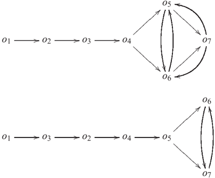
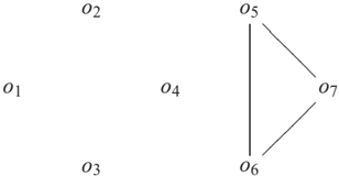
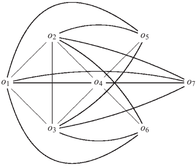
Example 1. Assume the set of all possible event occurrences is { oi : 1 ≤ i ≤ 7 } . The following is an example of a gso-structure, where

1. The earlier than relation is represented by a directed acyclic graph G 1:

/d40

/d35

/d59

/d54

Note that in this diagram, we used the solid edges to denote the edges of the transitive reduction 1 of the earlier than relation.

1 A transitive reduction of a binary relation R on a set X is a minimal relation R ′ on X such that the transitive closure of R ′ is the same as the transitive closure of R .

/d31

/d63

/d47

/d31

/d63

/d31

/d63

/d23

/d71

/d39

/d47

/d55

/d43

The not later than relation is represented as the following directed graph G 2:

/d40

/d35

/d59

/d109

/d54

Note that we used the dashed edges to denote the edges of G 2 which are not in G 1.

The nonsimultaneous relation is represented by the following (undirected) graph G 3 (because nonsimultaneous is symmetric).

Note that except the edge { o 2 , o 3 } , all other edges of G 3 are exactly the edges of the comparability graph of the earlier than relation. Because of the quantity of edges the comparability graph has, it is often more practical to draw the complement graph of the graph induced by the relation nonsimultaneous . For example,

/d31

/d63

/d47

/d31

/d63

/d31

/d63

/d23

/d71

/d12

/d31

/d39

/d47

/d55

/d43

/d24

/d70

the complement graph ¯ G 3 of the graph G 3 is the following:

/squaresolid

2.3 Observations and the observed before , observed simult relations

If the relations of a gso-structure in the previous section describe the specification level (also called structural semantics) of a concurrent system, observations characterize behavioral level of the system. The observed before (or observed simult ) relation relates two event occurrences and an observation.

Formula not decoded

Each observation and the observed before relation specify a stratified order on the event occurrences as follows. Every event occurrence cannot be observed before itself with respect to any observation.

Formula not decoded

The observed before is transitive with respect to any observation.

Formula not decoded

The observed simult relation and observed before can be derived from each other.

/negationslash

Formula not decoded

The observed before relation on a fixed observation satisfies the stratified order property.

Formula not decoded

Every observation and the observed before relation specify a stratified order extension of the gso-structure.

Formula not decoded

Axioms (2.21) and (2.22) impose the observation soundness property of our gso-structure theory in the following sense: if o is an possible observation of the system, then it must satisfy the constraints specified by the relations of the gso-structure.

We next axiomatize the observation completeness property of our gso-structure theory. If o 1 and o 2 are simultaneous event occurrences, then there must be some observation o , where o 1 and o 2 are observed simultaneously.

Formula not decoded

And if it is not the case that the event occurrence o 1 is not later than the event occurrence o 2, then there will be some observation o , where o 2 is observed earlier than o 1.

Formula not decoded

The reason why stratified orders are used to encode observations can be explained formally in the next two propositions.

For any observation o , we define:

Formula not decoded

Proposition 4. For all event occurrences o 1 , o 2 and o 3 , we have

1. o 1 /similarequal o o 2 2. o 1 /similarequal o o 2 ⊃ o 2 /similarequal o o 1 3. o 1 /similarequal o o 2 ∧ o 2 /similarequal o o 3 ⊃ o 1 /similarequal o o

In other words, the relation /similarequal o is an equivalence relation.

Proof. 1. Follows from how /similarequal o is defined.

Follows from axiom (2.19) and how /similarequal o is defined.
Follows from axiom (2.20) and how /similarequal o is defined.

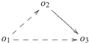
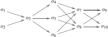
The intuition of Proposition 4 is that for any fixed observation o , we can extend the observed simult relation with the identity relation to construct the equivalence relation /similarequal o . The relation /similarequal o can then be used to partition the set of event occurrences, where we can think of each equivalence class as a 'composite event occurrence' consisting of only atomic event occurrences that are pairwise observed simultaneously within o . For example, Fig. 2.3 shows a stratified order ✁ o induced by an observation o and the observed before relation. In this case, the equivalence classes of /similarequal o are the sets { o 1 , o 2 } , { o 3 } , { o 4 , o 5 , o 6 } , { o 7 , o 8 } and { o 9 , o 10 } , where the fact that o 1 and o 2 belong to the same equivalence class means they are observed simultaneously within o .

/d58

/d36

Fig. 1: A example of a stratified order ✁ o induced by an observation o and the observed before relation. (Edges resulted from transitivity are omitted in this diagram for simplicity.)

Proposition 5. If A and B are two distinct equivalence classes of /similarequal o, then either A × B ⊆ ✁ o or B × A ⊆ ✁ o.

Proof. We pick a ∈ A and b ∈ B . Clearly, a ✁ o b or b ✁ o a , otherwise a /slurabove o b which contradicts that a , b are elements from two distinct equivalence classes. There are two cases:

If a ✁ o b : we want to show A × B ⊆ ✁ o . Let c ∈ A and d ∈ B , it suffices to show c ✁ o d . Assume for contradiction that ¬ ( c ✁ o d ) . Since c /negationslash/similarequal o d , it follows that d ✁ o c . There are three different subcases:
(a) If a = c , then d ✁ o a and a ✁ o b . Hence, d ✁ o b . This contradicts that d , b ∈ B .
(b) If b = d , then b ✁ o c and a ✁ o b . Hence, a ✁ o c . This contradicts that a , c ∈ A .

/negationslash

(c) If a = c and b = d , then a /slurabove o c and b /slurabove o d and ¬ ( a /slurabove o d ) and ¬ ( c /slurabove o b ) . Since ¬ ( a /slurabove o d ) , either a ✁ o d or d ✁ o a .

/negationslash

-If a ✁ o d : since d ✁ o c , it follows a ✁ o c . This contradicts a /slurabove o c .
-If d ✁ o a : since a ✁ o b , it follows d ✁ o b . This contradicts d /slurabove o b .

Therefore, we conclude A × B ⊆ ✁ o .

If b ✁ o a : using a symmetric argument, it follows that B × A ⊆ ✁ o . /intersectionsq /unionsq

Proposition 5 leads to the following consequence. For any observation o , let us define the relation ̂ ✁ o on the set Eo = { [ a ] /similarequal o : event occurrence ( a ) } as

Formula not decoded

/d42

/d52

/d47

/d42

/d52

/d42

/d52

/d63

/d31

/d47

/d36

/d47

/d58

Then the relation ̂ ✁ o is a strict total order on Eo . Intuitively, the equivalence classes in Eo can always be totally ordered using ̂ ✁ o , where for any two equivalence classes A and B in Eo , if A ̂ ✁ o B , then all event occurrences in A are observed before all the event occurrences in B within the observation o .

Formula not decoded

For examples, the equivalence classes of the stratified order from Fig. 2.3 can be totally ordered by the ordering ̂ ✁ o as follows:

When the cardinality of the set of event occurrences is finite as in our example, the stratified order from Fig. 2.3 can be equivalently represented more compactly as

Formula not decoded

where each equivalence class is called a step and the whole sequence is called a step sequence .

It might seem counterintuitive that our axioms allow observations whose infinitely many event occurrences are observed simultaneously. However, this is just a limitation of first order theory. Since our theory allows models that observe arbitrarily large finite set of simultaneous event occurrences, by the compactness theorem there will be models whose observations will allow us to observe infinite set of simultaneous event occurrences.

Observation soundness We have just discussed the idea behind why stratified orders are used to formalize the notion of an observation. We next want to show the intuition of how stratified order based observations satisfy the observation soundness properties with respect to a gso-structure. We will do so using a detailed example.

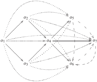
Example 2. Given the set of event occurrences { oi | 1 ≤ i ≤ 7 } and the relations earlier than , not later than and nonsimultaneous from Example 1, we want to know possible observations of this gso-structure. By axioms (2.21) and (2.22) for observation soundness, we know that all of the observations must satisfy all the causality constraints specified by these three relations. For each observation ob , we let Gob denote the dag representing the stratified order ✁ ob .

The observation ob satisfies the not later than relation intuitively meaning that Gob must contain G 1, i.e., G 1 ⊆ Gob .
The observation ob satisfies the not later than relation roughly which means that Gob might or might not contains the edges of G 2 -G 1, where G 2 -G 1 denotes the graph difference of G 2 and G 1. The exception is when G 2 -G 1 contains both directed edges ( oi , oj ) and ( oj , oi ) , then neither ( oi , oj ) nor ( oj , oi ) is allowed to be included in Gob .
Finally ob satisfies the nonsimultaneous relation is equivalent to saying that if { oi , oj } ∈ G 3, but neither ( oi , oj ) nor ( oj , oi ) is in the graph G 1, then we have the case that either ( oi , oj ) or ( oj , oi ) must be included in Gob .

From these intuitions, if earlier than , not later than and nonsimultaneous are given an interpretation as in Example 1, then we notice the follows.

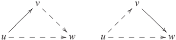
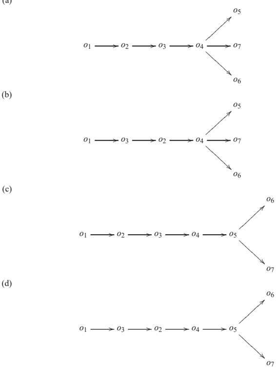
-Since ( o 3 , o 2 ) ∈ G 3 and ( o 2 , o 3 ) , ( o 3 , o 2 ) /negationslash∈ G 1, if we consider only the set of event occurrences { o 1 , o 2 , o 3 , o 4 } , then the transitive reduction graphs of all of the possible ways they can be observed are:

/d47

Formula not decoded

/d47

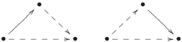
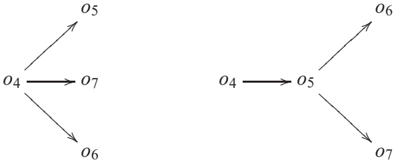
-Since ( o 5 , o 6 ) , ( o 5 , o 7 ) , ( o 7 , o 6 ) , ( o 6 , o 7 ) ∈ G 2 -G 1, if we consider only the set of event occurrences { o 4 , o 5 , o 6 , o 7 } , then the transitive reduction graphs of all of the possible ways they can be observed are:

/d62

/d32

Note that because ( o 7 , o 6 ) , ( o 6 , o 7 ) ∈ G 2 -G 1, the vertices o 6 are o 7 disconnected (incomparable) in all of the possible observations.

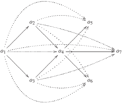
Combining all of these cases together, the transitive reduction graphs of all possible observations which satisfy the observation soundness condition with respect to the gsostructure from Example 1 are depicted in Fig. 2. /squaresolid

Observation completeness One subtle question one might ask is if the observation completeness condition is too strong for every gso-structure to have. In other words, is there any model of our theory, where its gso-structure cannot be characterized by any set of stratified order observations? Fortunately, the theorem which we will discuss next will help us answer this question. Before stating the theorem, let us define some notations.

For a partial order ✁ on a set X , let us define

Formula not decoded

The following theorem can be seen as a generalization of Szpilrain's theorem [17]. If Szpilrajn's Theorem ensures that every partial order can be uniquely reconstructed from the set of all of its total order extensions, then the following theorem states that every gso-structure can be uniquely reconstructed from its stratified order extensions.

/d47

/negationslash

/d47

(a)

/d32

Fig. 2: Transitive reduction graphs of all possible observations which satisfy the observation soundness condition with respect to the gso-structure from Example 1.

Theorem 1 (Guo and Janicki [2]). Let

be a gso-structure, i.e., M satisfies all axioms from (2.9) to (2.14) . Let Ω be the set of all stratified orders ✁ on X satisfying the following stratified order extension conditions:

nonsimultaneous M ⊆ ✁ /arrowparrleftright and
not later than M ⊆ ✁ /slurabove .

/d47

/d32

/d62

/d32

/d62

/d32

Then we have

/d47

nonsimultaneous

/d47

✁

⋂

/intersectionsq

/unionsq

From this theorem, we know that there is always a subset of Ω , where we can uniquely reconstruct not later than M and nonsimultaneous M . Note that although the consequence of the theorem does not mention earlier than M , the axiom (2.11) implies that

Formula not decoded

Thus, earlier than M = (⋂ ✁ ∈ Ω ✁ /arrowparrleftright ) ∩ (⋂ ✁ ∈ Ω ✁ /slurabove ) = ⋂ ✁ ∈ Ω ✁ . Hence, observation completeness is a safe assumption for our gso-structure theory.

It is worth noticing that, since Theorem 1 is a generalization of Szpilrajn's Theorem, the proof of Theorem 1 requires the axiom of choice .

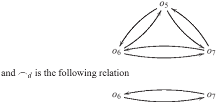
Example 3. Let ✁ a , ✁ b , ✁ c and ✁ d be the stratified orders whose transitive reduction graphs are depicted in cases (a), (b), (c) and (d) respectively. Then the set of all the stratified order extensions of the gso-structure from Example 1 is Ω = { ✁ a , ✁ b , ✁ c , ✁ d } . However, the gso-structure from Example 1 can be uniquely reconstructed from any subset of Ω , which is a superset of at least one of the following two sets { ✁ a , ✁ d } and { ✁ b , ✁ c } .

For example, let us consider the set { ✁ a , ✁ d } . Then the relations ✁ /slurabove a and ✁ /slurabove d can be represented as the following two graphs (some arcs which can be inferred from transitivity are omitted for simplicity):

/d62

/d83

/d109

/d19

/d32

It is easy to check that the graph G 2 is exactly the intersection of these two graphs. It is also easy to check that the graph G 3 is the intersection of the comparability graphs induced by the relations ✁ a and ✁ d . /squaresolid

Let T gso denote our gso-structure theory, which consists of axioms from (2.1) to (2.24). Then we have the following theorem.

Theorem 2. The theory T gso is consistent.

∈

✁

/arrowparrleftright

/d47

and not later than

/d47

/d32

/d19

/d113

/d62

/d32

/d62

/d83

✁

∈

✁

/slurabove

Proof. It suffices to build a model M that satisfies all of these axioms. Let E , EO and O be three pairwise disjoint sets, where

Formula not decoded

We define the universe of M to be the set U df = E ∪ EO ∪ O . We then give the following interpretations

event M = E
event occurrence M = EO
observation M = O
occurrence M = { ( ei , oi ) : 1 ≤ i ≤ 7 }
not later than M is exactly the graph G 2 from Example 1
earlier than M is exactly the graph G 1 from Example 1
nonsimultaneous M is exactly the graph G 3 from Example 1
observed simult M = { ( o 1 , o 2 , oba ) : o 1 /slurabove a o 2 }∪{ ( o 1 , o 2 , obd ) : o 1 /slurabove d o 2 } , where /slurabove a is the following relation
observed before M = { ( o 1 , o 2 , oba ) : o 1 ✁ a o 2 } ∪ { ( o 1 , o 2 , obd ) : o 1 ✁ d o 2 } , where ✁ a and ✁ d are relations from Example 3.

/d70

/d102

/d50

/d114

It is easy to check that axioms (2.1) to (2.5) are satisfied by this interpretation. We also see from Example 1 how the interpretation of earlier than , not later than and nonsimultaneous given by G 1, G 2 and G 3 respectively satisfies that axioms from (2.6) to (2.14). It is also clear from Example 2 and Example 3 that our interpretation satisfies axioms from (2.15) to (2.24). /intersectionsq /unionsq

3 Models of the theory T gso

By Theorem 2, we already know that T gso is consistent, and hence the class of all models satisfying T gso is nonempty. In this section, we will attempt to classify all the possible models of our theory T gso . For convenience, we let T univ denote the theory consisting of axioms from (2.1) to (2.5), and we let T spec denote the specification-level theory consisting of axioms from (2.6) to (2.14).

/d6

/d114

/d38

/d50

3.1 Events and their occurrences

The following definition will give us the classification of all models of T univ .

Definition 1. Let M univ denote the class of all possible models for T univ. Then any model M ∈ M univ consists of the following sets E, EO, and O such that

the universe M of M is E ∪ EO ∪ O 2. E, EO, and O are pairwise disjoint 3. E is a partitioning of the set EO. 4. E = event M 5. EO = event occurrence M 6. O = observation M 7. occurrence M = { ( x , e ) ∈ EO × E : x ∈ e }

/squaresolid

The correctness of our definition follows from the following theorem.

Theorem 3 (Satisfiability Theorem for T univ ). If the class M univ is defined as in Definition 1, then for any model M ∈ M univ , we have M | = T univ .

Proof. The fact that M satisfies axioms (2.1) and (2.2) follows from the condition that E , EO , and O are pairwise disjoint. The fact that M satisfies axioms (2.3) and (2.5) follows from our construction that E is a partitioning of the set EO and the interpretation of occurrence as the membership relation between EO and E . /intersectionsq /unionsq

Theorem 4 (Axiomatizability Theorem for T univ ). Any model of T univ is isomorphic to a structure of M univ .

Proof. Let M be a model of T univ . We will show that M satisfies the conditions of the structures in M univ from Definition 1.

Since M | = (2.1) , we know that any element of the universe M of M belongs to one of the following sets event M , event occurrence M and observation M . Since M | = (2.2), all of these sets event M , event occurrence M and observation M are pairwise disjoint. Hence, the conditions (1), (2), (4)-(6) are satisfied.

Since M satisfied axioms (2.3)-(2.4), we know that occurrence M a function

Formula not decoded

Hence, given the set EO = event occurrence M , we can define the set E as

Formula not decoded

Since occurrence M is a function, it can be easily checked that E defines a partitioning of EO . Thus, the condition (3) and (7) are also satisfied. /intersectionsq /unionsq

3.2 Graph-theoretic classification of gso-structures

We will classify the relational models of T spec in a more well-understood combinatorial setting. But before that we will recall some definitions.

Definition 2. A directed graph G is a pair ( V , E ) , where V is the set of vertices and E ⊆ V × V \{ ( v , v ) ∈ V × V } is the set of edges.

-The transitive closure of G is a graph G + = ( V , E + ) such that for all v , w in V there is an edge ( v , w ) in E + if and only if there is a nonempty path from v to w in G.
-The graph G is called a transitive graph if we have E = E + \{ ( v , v ) ∈ E + } . In other words, G is its own transitive-closure taken away all the self-loops.
-We let C ( G ) = ( V , C ( E )) denote the comparability graph of G, i.e.,

Formula not decoded

-We let IC ( G ) = ( V , IC ( E )) denote the incomparability graph of G, i.e.,

Formula not decoded

-We let G =( V , E ) denote the complement graph of G, i.e.,

Formula not decoded

/negationslash

In other words, we exclude the self-loops.

-Given a directed graph H =( V , E ′ ) , we write G ⊆ H if E ⊆ E ′ . We write G -H to denote the graph ( V , E \ E ′ ) . And we write G ∪ H to denote the graph ( V , E ∪ E ′ ) .

/squaresolid

In this paper, we will treat undirected graphs (or graphs) as a special case of directed graph, where the edge relations are symmetric. This explains why we defined C ( G ) and IC ( G ) as direct graphs. Also note that whenever we call something a graph or a directed graph, we already mean that it does not contain any self-loop.

Definition 3. Let M spec denote the class of all possible models for T spec. Then any model M ∈ M univ can be uniquely determined from the following three graphs:

The graph G 1 =( EO , E 1 ) is a acyclic transitive graph.
The graph G 2 =( EO , E 2 ) is a transitive graph satisfying the following two conditions:
(a) G 2 = G 1 ∪ G 3 , where G 3 ⊆ IC ( G 1 ) .
(b) the graph G 2 does not contain a triangle that has any of these two forms:

/d63

/d95

/d31

/d47

/d95

/d31

/d47

/d95

/d63

/d95

where the solid edges are edges of G 1 and the dashed edges are edges of G 3 .

The graph G 4 = ( EO , E 4 ) is an undirected graph such that there is an undirected graph G 5 ⊆ IC ( G 2 ) and G 4 = C ( G 1 ) ∪ G 5 .

The interpretation for M can be defined as:

-the universe M of M is a superset of EO
-event occurrence M = EO
-not later than M = E 2
-earlier than M = E 1
-nonsimultaneous M = E 4 .

This is a contradiction.

/d47

/d32

/squaresolid

Theorem 5 (Satisfiability Theorem for T spec ). If the class M spec is defined as in Definition 3, then for any model M ∈ M spec , we have M | = T spec.

Proof. Since earlier than M , not later than M and nonsimultaneous M are exactly the edge relations of G 1, G 2 and G 3 respectively, it follows that M satisfies axioms (2.6)(2.8).

Since nonsimultaneous M = E 4 and G 4 is a graph, it follows that M satisfies axioms (2.9) and (2.10).

Recall that we define earlier than M = E 1 and not later than M = E 2. Hence, to show that M | = (2.11), it suffices to show the following lemma.

Lemma 1. G 1 = G 2 ∩ G 4 .

Proof (Proof of Lemma 1). ( ⊆ ) From Definition 3, we know that G 4 = C ( G 1 ) ∪ G 5 and G 2 = G 1 ∪ G 3. Hence, it follows that C ( G 1 ) ∩ G 1 ⊆ G 4 ∩ G 1. But we know that G 1 = C ( G 1 ) ∩ G 1.

( ⊇ ) It suffices to show that G 5 ∩ G 2 = / 0 and G 3 ∩ G 4 = / 0. But we know that G 5 ∩ G 2 = / 0 since from condition (3) of Definition 3, we have G 5 ⊆ IC ( G 2 ) . This also implies that that G 3 ∩ G 5 = / 0. It remains to show that G 3 ∩ C ( G 1 ) = / 0, but this holds since from condition (2)(a) of Definition 3 we have G 3 ⊆ IC ( G 1 ) . /intersectionsq /unionsq

Since G 2 is a transitive graph, it follows that M satisfies axioms (2.12) and (2.13). It remains to show that M | = (2.14). Then since G 2 = G 1 ∪ G 3, there are three cases to consider:

-If ( o 1 , o 2 ) ∈ E 1 and ( o 2 , o 3 ) ∈ E 1, then it follows that ( o 1 , o 3 ) ∈ E 1 since G 1 is a transitive graph.
-If ( o 1 , o 2 ) ∈ E 3 and ( o 2 , o 3 ) ∈ E 1, where E 3 is the set of edges of G 3, then since G 2 is a transitive graph, we know that ( o 1 , o 3 ) ∈ E 2. Suppose for a contradiction that ( o 1 , o 3 ) ∈ E 3, then we have a triangle

/d62

-The case of ( o 1 , o 2 ) ∈ E 1 and ( o 2 , o 3 ) ∈ E 3 is similar to the previous case.

/d95

/intersectionsq /unionsq

Theorem 6 (Axiomatizability Theorem for T spec ). Any model of T spec is isomorphic to a structure of M spec .

Proof. Let M be a model of T spec . We will show that M satisfies the conditions of the structures in M spec from Definition 3.

Since M satisfies axioms (2.6) and (2.7), we know that we can determine the vertex set EO = event occurrence M for the graphs G 1, G 2 and G 3.

Since M satisfies all axioms, from Proposition 1 we know that earlier than M is a strict partial order, so it can be represented by an acyclic transitive graph G 1 as from the condition (1) of Definition 3.

Since M satisfies axioms (2.12) and (2.13), we can represent the not later than M relation by a transitive graph G 2 as from the condition (2) of Definition 3.

-To show that the condition (2)(a) is satisfied, we must show that G 3 = G 2 -G 1 ⊆ IC ( G 1 ) . Suppose for a contradiction that there is an edge ( u , v ) that appears on both G 3 and IC ( G 1 ) . Since G 3 = G 2 -G 1, we know that ( u , v ) /negationslash∈ E 1, so ( v , u ) ∈ E 1. This would mean that earlier than M ( v , u ) and not later than M ( u , v ) . But this contradicts with Proposition 3.
-To show that the condition (2)(b) is satisfied, we assume for a contradiction that we have at least one of the following two triangles:

/d63

/d95

/d31

/d47

/d95

/d31

/d47

/d95

/d63

/d95

where the solid edges are edges of G 1 and the dashed edges are edges of G 3. The left triangle implies that earlier than M ( u , v ) and not later than M ( v , w ) but not later than M ( u , w ) . This contradicts with axiom (2.14). Similarly the case of the right triangle also leads to a contradiction.

Since M satisfies axioms (2.9) and (2.10), we can represent nonsimultaneous M by a graph G 4 as from the condition (3) of Definition 3. Let G 5 = G 4 -C ( G 1 ) , it remains to show that G 5 ⊆ IC ( G 2 ) . Suppose for a contradiction that an edge ( u , v ) and ( v , u ) is shared by both the graph G 5 and C ( G 2 ) . Without loss of generality, we can assume that ( u , v ) ∈ G 2. Thus, not later than M ( u , v ) and nonsimultaneous M ( u , v ) . But by axiom (2.11), we have that earlier than M ( u , v ) . This contradicts with our assumption that ( u , v ) ∈ G 5 = G 4 -C ( G 1 ) . /intersectionsq /unionsq

3.3 Observations

We first introduce a more combinatorial representation of stratified orders.

Definition 4. Given a set X, we call the pair ( P , /triangleleftsld ) a ranking structure of X if P is a partitioning of the set X and /triangleleftsld is a total ordering on the set P. /squaresolid

Intuitively, a ranking structure of X is just a partitioning P of X equipped with a total ordering which orders the partitions in P .

Proposition 6. Any stratified order ✁ on a set X can be uniquely determined by a ranking structure of X.

Proof. Similarly to the ideas from Proposition 4 and Proposition 5, we define an equivalence relation from the stratified order ✁ as follows:

Formula not decoded

/negationslash

Then let P be the set of all partitions of X with respect to this equivalence relation /similarequal ✁ .

Next we define the relation /triangleleftsld as /triangleleftsld df = { ( A , B ) ∈ P × P : A × B ⊆ ✁ } . Then, similarly to Proposition 5, we can check that /triangleleftsld is a total ordering.

To recover the stratified order ✁ from the ranking structure ( P , /triangleleftsld ) , we simply reconstruct

/negationslash

Formula not decoded

For a set A , we let K ( A ) denote the complete graph induced by A . In other words, K ( A ) = ( A , E ) and

Formula not decoded

/negationslash

For each ranking structure R =( P , /triangleleftsld ) of a set X , we have two kinds of graph associated with it:

/negationslash

Formula not decoded

Intuitively, the graph G ( R ) is simply the transitive graph of the stratified order encoded by R . And the graph ⋃ A ∈ P K ( A ) is exactly the graph IC ( G ( R )) , but in this case it is more intuitive to characterize it as the union of complete graphs.

Putting everything together we have the following characterization of the class of all models of T gso .

Definition 5. Let M gso denote the class of all possible models for T gso. Then any model M ∈ M gso is uniquely determined from

-the sets E, EO, and O
-the graphs G 1 , G 2 and G 3
-a family F of ranking structures on EO indexed by the set O, i.e., F = { Ro : o ∈ O } ,

such that

all conditions from Definition 1 are satisfied

all conditions from Definition 3 are satisfied
observed before M = { ( x , y , o ) : ( x , y ) is an edge of the graph G ( Ro ) }
the graph G 2 is the intersection of all the graphs in the set { ̂ G ( Ro ) : o ∈ O } 4. the graph G 3 is the intersection of all the graphs in the set { C ( G ( Ro )) : o ∈ O }
observed simult M = { ( x , y , o ) : ( x , y ) is an edge of the graph ⋃ A ∈ Ro K ( A ) }

/squaresolid

Theorem 7 (Satisfiability Theorem for T gso ). If the class M gso is defined as in Definition 5, then for any model M ∈ M gso , we have M | = T gso.

Proof. The fact that M satisfies axioms (2.1) and (2.5) follows from the Theorem 3. The fact that M satisfies axioms (2.6) and (2.14) follows from the Theorem 5.

Since each Ro is a ranking structure on EO , from the way observed before M and observed simult M are defined, we know that M satisfies axioms (2.15) and (2.16).

Since observed simult M is defined from the graphs ⋃ A ∈ Ro K ( A ) and each graph ⋃ A ∈ Ro K ( A ) is the incomparability graph of G ( Ro ) , it follows that M | = (2.19). Also since we construct the observed before M relation from the graphs G ( Ro ) and each G ( Ro ) is a stratified order. Hence, M satisfies axioms (2.17), (2.18) and (2.20) since these axioms are the conditions saying that ✁ o is a stratified order for every o and we have G ( Ro ) = ✁ o .

Recall axioms (2.21)-(2.24) together say that

Formula not decoded

But this is equivalent to conditions (2) and (3) from Definition 5.

/intersectionsq /unionsq

Theorem 8 (Axiomatizability Theorem for T gso ). Any model of T gso is isomorphic to a structure of M gso .

Proof. Let M be a model of T gso . We will show that M satisfies the conditions of the structures in M gso from Definition 3.

Since M satisfies axioms (2.1)-(2.5), from Theorem 4 we can determine the sets E = event M and the set EO = event occurrence M , which satisfied the condition (1) of Definition 5.

Since M satisfies axioms (2.6)-(2.14), from Theorem 6 we can determine the graphs G 1, G 2 and G 3 such that the condition (2) of Definition 5 is satisfied.

Let O = event occurrence M . Then since M satisfies axioms (2.15)-(2.20), we know that for all o the induced relation ✁ o is a stratified order, so we can uniquely construct the family of ranking structure F = { Ro : o ∈ O } from the set { ✁ o : o ∈ O } . It is easy to check that the condition (5) and (6) of Definition 5 are satisfied.

But since we already know that axioms (2.21)-(2.24) together are equivalent to conditions (3.1) and (3.2) from the proof of Theorem 7, it follows that M satisfies conditions (2) and (3) of Definition 5. /intersectionsq /unionsq

4 A semantic mapping to PSL-core

In this section, we will attempt to map a subset of T gso to the PSL-core theory ( T pslcore ). We let T -gso to denote the theory consisting of axioms from (2.6) to (2.24) and the following two axioms.

Formula not decoded

Axiom (4.1) says that everything is either an event occurrence or an observation . And axiom (4.2) says that the set of event occurrences and the set of observations are disjoint.

The reason for considering the theory T -gso is that all of the interesting properties of T gso concern with event occurrences and not with the events themselves. The second reason is that beside weakening the theory T gso , we do not see how we can establish a semantic mapping from T gso to T pslcore without introducing extra axioms into T pslcore .

To shorten our formulas, we need the following notation. For any formula P ( x ) we define

In other words, we write ( ∃ ! x ) P ( x ) to say that there exists a unique x satisfying P ( x ) .

Formula not decoded

Definition 6 (Interpretation of T -gso into T pslcore ). We let π denote the relative interpretation of the language of T -gso into T pslcore. Then the interpretation π is defined as follows:

Formula not decoded

Intuitively, the interpretation means the following. If in T -gso each observation is a 'system run', encoded by a stratified order of the event occurrences, which is observed by some implicit observer, then in T pslcore we explicitly describe this observer as an object. For our interpretation, we are particularly interested in objects that participate in a unique activity occurrence of each activity at a unique time point. In other words, observers are objects satisfying the following properties:

The time point in which an object participates with an activity occurrence of an activity is exactly the time when the object observes the activity.
The object observes every activity.
The object only observes each activity exactly once.

All of the other interpretations π earlier than , π not later than and π nonsimultaneous can be easily determined from the observations that all observers observed.

Theorem 9. The interpretation π defined in Definition 6 is correct.

Proof. It is easy to check that under the interpretation π , every axioms of T -gso is a theorem of T pslcore . Hence, π defined in Definition 6 is a correct interpretation. /intersectionsq /unionsq

5 Conclusion

In this paper, we proposed in our knowledge the first version of a first-order theory for gso-structures in [2,5]. We avoid the difficulty of not being able to quantify over relations in first-order logic by introducing the relations observed before and observed simult which take an observation as one of their parameters.

Using model-theoretic ontological techniques introduced in [4], we classified all possible models of T gso , where our key results are the satisfiability theorem and axiomatizability theorem for T gso . In our opinion, the classification of models of T spec , which decomposes the earlier than , not later than and nonsimultaneous into smaller graphs, is especially insightful in understanding these three relations. Although the classification of observations using ranking structures is quite artificial, we could not figure out any simpler characterization.

We also give a very intuitive interpretation of the weaker theory T -gso into T pslcore , which shows that T pslcore is strong enough to prove most of the theorems in T gso . The main philosophical difference between T gso and T pslcore is that causality relations are treated as logical relations without mentioning the concept of time in T gso while the

causality relations in T pslcore are directly connected to timepoints of a reference timeline.

The fact that T -gso can be correctly interpreted inside T pslcore also suggests that the soundness and completeness conditions might be too restrictive. One way to relax these conditions is to partition the observation set into 'legal' and 'illegal' observations, where legal observations are the ones satisfying the soundness and completeness conditions. This approach would also give us the ability to talk about illegal observations.

References

H. Gaifman and V. Pratt, Partial Order Models of Concurrency and the Computation of Function, Proc. of LICS'87 , pp. 72-85.
G. Guo and R. Janicki, Modelling Concurrent Behaviours by Commutativity and Weak Causality Relations, Proc. of AMAST'02, LNCS 2422 (2002), 178-191.
M. Gruninger, Ontology of the Process Specification Language, Handbook of Ontologies and Information Systems , S. Staab (ed.), Springer 2003, pp. 599-618.
M. Gruninger, The Model Theory of PSL-Core.
R. Janicki. Relational Structures Model of Concurrency. Acta Informatica , 45(4): 279-320, 2008.
R. Janicki and M. Koutny, Invariants and Paradigms of Concurrency Theory, LNCS 506, Springer 1991, pp. 59-74.
R. Janicki and M. Koutny, Structure of Concurrency, Theoretical Computer Science , 112(1):5-52, 1993.
R. Janicki and M. Koutny, Semantics of Inhibitor Nets, Information and Computation , 123(1):1-16, 1995.
R. Janicki and M. Koutny, Fundamentals of Modelling Concurrency Using Discrete Relational Structures, Acta Informatica , 34:367-388, 1997.
R. Janicki and M. Koutny, On Causality Semantics of Nets with Priorities, Fundamenta Informaticae 34:222-255, 1999.
G. Juh´ as, R. Lorenz, S. Mauser, Synchronous + Concurrent + Sequential = Earlier Than + Not Later Than, Proc. of ACSD'06 (Application of Concurrency to System Design), Turku, Finland 2006, pp. 261-272, IEEE Press.
G. Juh´ as, R. Lorenz, C. Neumair, Synthesis of Controlled Behavious with Modules of Signal Nets, LNCS 3099, Springer 2004, pp. 233-257.
Y. Kalfoglou and M. Schorlemmer, Ontology mapping: the state of the art, The Knowledge Engineering Review , 18(1):1-31, 2003.
H. C. M. Kleijn and M. Koutny, Process Semantics of General Inhibitor Nets, Information and Computation , 190:18-69, 2004.
D. T. M. Lˆ e, Studies in Comtrace Monoids, Masters Thesis, McMaster University, 2008.
M. Pietkiewicz-Koutny, The Synthesis Problem for Elementary Net Systems, Fundamenta Informaticae 40(2,3):310-327, 1999.
E. Szpilrajn, Sur l'extension de l'ordre partiel, Fundamenta Mathematicae 16 (1930), 386389.