Multi-Objective AI Planning: Evaluating DaEYAHSP on a Tunable Benchmark

M. R. Khouadjia 1 , M. Schoenauer 1 , V. Vidal 2 , J. Dr´ eo 3 , and P. Sav´ eant 3

1 TAO Project-team, INRIA Saclay & LRI, Universit´ e Paris-Sud, Orsay, France { mostepha-redouane.khouadjia,marc.schoenauer } @inria.fr , 2 ONERA-DCSD, Toulouse, France [email protected] THALES Research & Technology, Palaiseau, France johann.dreo, pierre.saveant } @thalesgroup.com

3 {

Abstract. All standard Artifical Intelligence (AI) planners to-date can only handle a single objective, and the only way for them to take into account multiple objectives is by aggregation of the objectives. Furthermore, and in deep contrast with the single objective case, there exists no benchmark problems on which to test the algorithms for multi-objective planning.

Divide-and-Evolve ( DaE ) is an evolutionary planner that won the (singleobjective) deterministic temporal satisficing track in the last International Planning Competition. Even though it uses intensively the classical (and hence single-objective) planner YAHSP ( Yet Another Heuristic Search Planner ), it is possible to turn DaEYAHSP into a multi-objective evolutionary planner.

A tunable benchmark suite for multi-objective planning is first proposed, and the performances of several variants of multi-objective DaEYAHSP are compared on different instances of this benchmark, hopefully paving the road to further multi-objective competitions in AI planning.

1 Introduction

An AI Planning problem (see e.g. [1]) is defined by a set of predicates, a set of actions, an initial state and a goal state. A state is a set of non-exclusive instantiated predicates, or (Boolean) atoms. An action is defined by a set of pre-conditions and a set of effects : the action can be executed only if all preconditions are true in the current state, and after an action has been executed, the effects of the action modify the state: the system enters a new state. A plan in AI Planning is a sequence of actions that transforms the initial state into the goal state. The goal of AI Planning is to find a plan that minimizes some quantity related to the actions: number of actions, or sum of action costs in case actions have different costs, or makespan in the case of temporal planning, when actions have a duration and can eventually be executed in parallel. All these problems are P-SPACE.

This work was partially funded by DESCARWIN ANR project (ANR-09-COSI-002).

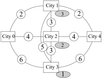
A simple planning problem in the domain of logistics is given in Figure 1: the problem involves cities, passengers, and planes. Passengers can be transported from one city to another, following the links on the figure. One plane can only carry one passenger at a time from one city to another, and the flight duration (number on the link) is the same whether or not the plane carries a passenger (this defines the domain of the problem). In the simplest non-trivial instance of such domain, there are 3 passengers and 2 planes. In the initial state, all passengers and planes are in city 0 , and in the goal state, all passengers must be in city 4 . The not-so-obvious optimal solution has a total makespan of 8 and is left as a teaser for the reader.

AI Planning is a very active field of research, as witnessed by the success of the ICAPS conferences ( http://icaps-conferences.org ), and its Intenational Planning Comptetition (IPC), where the best planners in the world compete on a set of problems. This competition has lead the researchers to design a common language to describe planning problems, PDDL (Planning Domain Definition Language). Two main categories of planners can be distinguished: exact planners are guaranteed to find the optimal solution . . . if given enough time; satisficing planners give the best possible solution, but with no optimality guarantee. A complete description of the state-of-the-art planners is far beyond the scope of this paper.

However, to the best of our knowledge, all existing planners are single objective (i.e. optimize one criterion, the number of actions, the cost, or makespan, depending on the type of problem), whereas most real-world problems are in fact multi-objective and involve several contradictory objectives that need to be optimized simultaneously. For instance, in logistics, the decision maker must generally find a trade-off between duration and cost (or/and risk).

An obvious solution is to aggregate the different objectives into a single objective, generally a fixed linear combination of all objectives. Early work in that area used some twist in PDDL 2.0 [2,3,4]. PDDL 3.0, on the other hand, explicitly offered hooks for several objectives x, and a new track of IPC was dedicated to aggregated multiple objectives: the 'net-benefit' track took place in 2006 [5] and 2008 [6], . . . but was canceled in 2011 because of the small number of entries. In any case, no truly multi-objective approach to multi-objective planning has been proposed since the very preliminary proof-of-concept in the first Divide-and-Evolve paper [7].

One goal of this paper is to build on this preliminary work, and to discuss various issues related to the challenge of solving multi-objective problems with an evolutionary algorithm that is heavily based on a single-objective planner ( YAHSP [8]) - and in particular to compare different state-of-the-art multiobjective evolutionary schemes when used within DaEYAHSP . However, experimental comparison requires benchmark problems. Whereas the IPC have validated a large set of benchmark domains, with several instances of increasing complexity in each domain, nothing yet exists for multi-objective planning. The other goal of this paper is to propose a tunable set of benchmark instances, based on a simplified model of the IPC logistics domain Zeno illustrated in Fig. 1. One advantage of this multi-objective benchmark is that the exact Pareto Front is known, at least for its simplest instances.

The paper is organized as follows: Section 2 rapidly introduces Divide-andEvolve , more precisely the representation and variation operators that have been used in the single-objective version of DaEYAHSP that won the temporal deterministic satisficing track at the last IPC in 2011. Section 4 details the proposed benchmark, called MultiZeno , and gives hints about how to generate instances of different complexities within this framework. Section 3.2 rapidly introduces the 4 variants of multi-objective schemes that will be experimentally compared on some of the simplest instances of the MultiZeno benchmark and results of different series of experiments are discussed in Section 6. Section 7 concludes the paper, giving hints about further research directions.

2 Divide-and-Evolve

Let P D ( I, G ) denote the planning problem defined on domain D (the predicates, the objects, and the actions), with initial state I and goal state G . In STRIPS representation model [9], a state is a list of Boolean atoms defined using the predicates of the domain, instantiated with the domain objects.

In order to solve P D ( I, G ), the basic idea of DaEX is to find a sequence of states S 1 , . . . , S n , and to use some embedded planner X to solve the series of planning problems P D ( S k , S k +1 ), for k ∈ [0 , n ] (with the convention that S 0 = I and S n +1 = G ). The generation and optimization of the sequence of states ( S i ) i ∈ [1 ,n ] is driven by an evolutionary algorithm. After each of the sub-problems P D ( S k , S k +1 ) has been solved by the embedded planner, the concatenation of the corresponding plans (possibly compressed to take into account possible parallelism in the case of temporal planning) is a solution of the initial problem. In case one sub-problem cannot be solved by the embedded solver, the individual is said unfeasible and its fitness is highly penalized in order to ensure that feasible individuals always have a better fitness than unfeasible ones, and are selected only when there are not enough feasible individual. A thorough description of DaEX can be found in [10]. The following rest of this section will focus on the evolutionary parts of DaEX .

2.1 Representation and Initialization

An individual in DaEX is hence a variable-length list of states of the given domain. However, the size of the space of lists of complete states rapidly becomes untractable when the number of objects increases. Moreover, goals of planning problems need only to be defined as partial states, involving a subset of the objects, and the aim is to find a state such that all atoms of the goal state are true. An individual in DaEX is thus a variable-length list of partial states, and a partial state is a variable-length list of atoms.

Previous work with DaEX on different domains of planning problems from the IPC benchmark series have demonstrated the need for a very careful choice of the atoms that are used to build the partial states [11]. The method that is used today to build the partial states is based on a heuristic estimation, for each atom, of the earliest time from which it can become true [12]. These earliest start times are then used in order to restrict the candidate atoms for each partial state: the number of states is uniformly drawn between 1 and the number of estimated start times; For every chosen time, the number of atoms per state is uniformly chosen between 1 and the number of atoms of the corresponding restriction. Atoms are then added one by one: an atom is uniformly drawn in the allowed set of atoms (based on earliest possible start time), and added to the individual if it is not mutually exclusive (in short, mutex ) with any other atom that is already there. Note that only an approximation of the complete mutex relation between atoms is known from the description of the problem, and the remaining mutexes will simply be gradually eliminated by selection, because they make the resulting individual unfeasible.

To summarize, an individual in DaEX is represented by a variable-length time-consistent sequence of partial states, and each partial state is a variablelength list of atoms that are not pairwise mutex.

2.2 Variation Operators

Crossover and mutation operators are defined on the DaEX representation in a straightforward manner - though constrained by the heuristic chronology and the partial mutex relation between atoms.

A simple one-point crossover is used, adapted to variable-length representation: both crossover points are independently chosen, uniformly in both parents. However, only one offspring is kept, the one that respects the approximate chronological constraint on the successive states. The crossover operator is applied with a population-level crossover probability.

Four different mutation operators are included: first, a population-level mutation probability is used; one an individual has been designated for mutation, the choice between the four mutation operators is made according to user-defined relative weights. The four possible mutations operate either at the individual level, by adding (addState) or removing (delState) a state, or at the state level by adding (addAtom) or removing (delAtom) some atoms in a uniformly chose state.

All mutation operators maintain the approximate chronology between the intermediate states (i.e., when adding a state, or an atom in a state), and the local consistency within all states (i.e. avoid pairwise mutexes).

2.3 Hybridization

DaEX uses an external embedded planner to solve the sequence of sub-problems defined by the ordered list of partial states. Any existing planner can in theory be used. However, there is no need for an optimality guarantee when solving the intermediate problems in order for DaEX to obtain good quality results [10]. Hence, and because several calls to this embedded planner are necessary for a single fitness evaluation, a sub-optimal but fast planner is used: YAHSP [8] is a lookahead strategy planning system for sub-optimal planning which uses the actions in the relaxed plan to compute reachable states in order to speed up the search process.

For any given k , if the chosen embedded planner succeeds in solving P D ( S k , S k +1 ), the final complete state is computed by executing the solution plan from S k , and becomes the initial state of the next problem. If all the sub-problems are solved by the embedded planner, the individual is called feasible , and the concatenation of the plans for all sub-problems is a global solution plan for P D ( S 0 = I, S n +1 = G ). However, this plan can in general be further optimized by rescheduling some of its actions, in a step called compression. The computation of all objective values is done from the compressed plan of the given individual. Finally, because the rationale for DaEX is that all sub-problems should hopefully be easier than the initial global problem, and for computational performance reason, the search capabilities of the embedded planner YAHSP are limited by setting a maximal number of nodes that it is allowed to expand to solve any of the sub-problems (see again [10] for more details).

3 Multi-Objective Divide-and-Evolve

In some sense, the multi-objectivization of DaEX is straightforward - as it is for most evolutionary algorithms. The 'only' parts of the algorithm that require some modification are the selection parts, be it the parental selection, that chooses which individual from the population are allowed to breed, and the environmental selection (aka replacement), that decides which individuals among parents and offspring will survive to the next generation. Several schemes have been proposed in the EMOA literature (see e.g. Section 3.2), and the end of this Section will briefly introduce the ones that have been used in this work. However, a prerequisite is that all objectives are evaluated for all potential solutions, and the challenge here is that the embedded planner YAHSP performs its search based on only one objective.

3.1 Multi-objectivization Strategies

Even though YAHSP (like all known planners to-date) only solves planning problems based on one objective. However, it is possible since PDDL 3.0 to add some other quantities (aka Soft Constraints or Preferences [13]) that are simply computed throughout the execution of the final plan, without interfering with the search.

The very first proof-of-concept of multi-objective DaEX [7], though using an exact planner in lieu of the satisficing planner YAHSP , implemented the simplest idea with respect to the second objective: ignore it (though computing its value for all individuals) at the level of the embedded planner, and let the evolutionary multi-objective take care of it. However, though YAHSP can only handle one objective at a time, it can handle either one in turn, provided they are both defined in the PDDL domain definition file. Hence a whole bunch of smarter strategies become possible, depending on which objective YAHSP is asked to optimize every time it runs on a sub-problem. Beyond the fixed strategies, in which YAHSP always uses the same objective throughout DaEYAHSP runs, a simple dynamic randomized strategy has been used in this work: Once the planner is called for a given individual, the choice of which strategy to apply is made according to roulette-wheel selection based on user-defined relative weights; In the end, it will return the values of both objectives. It is hoped that the evolutionary algorithm will find a sequential partitioning of the problem that will nevertheless allow the global minimization of both objectives. Section 6.2 will experimentally compare the fixed strategies and the dynamic randomized strategy where the objective that YAHSP uses is chosen with equal probability among both objectives.

Other possible strategies include adaptive strategies, where each individual, or even each intermediate state in every individual, would carry a strategy parameter telling YAHSP which strategy to use - and this strategy parameter would be subject to mutation, too. This is left for further work.

3.2 Evolutionary Multi-Objective Schemes

Several Multi-Objective EAs (MOEAs) have been proposed in the recent years, and this work is concerned with comparing some of the most popular ones when used within the multi-objective version of DaEYAHSP . More precisely, the following selection/reproduction schemescan be applied to any representation, and will be experimented with here: NSGA-II [14], SPEA2 [15], and IBEA [16]. They will now be quickly introduced in turn.

The Non-dominated Sorting Genetic Algorithm (NSGA-II) has been proposed by Deb et al. [14]. At each generation, the solutions contained in the current population are ranked into successive Pareto fronts in the objective space. Individuals mapping to vectors from the first front all belong to the best efficient set; individuals mapping to vectors from the second front all belong to the second best efficient set; and so on. Two values are then assigned for every solution of the population. The first one corresponds to the rank of the Pareto front the corresponding solution belongs to, and represents the quality of the solution in terms of convergence. The second one, the crowding distance, consists in estimating the density of solutions surrounding a particular point in the objective space, and represents the quality of the solution in terms of diversity. A solution is said to be better than another solution if it has a better rank value, or in case of equality, if it has a larger crowding distance.

The Strength Pareto Evolutionary Algorithm (SPEA) [17], introduces an improved fitness assignment strategy. It intrinsically handles an internal fixedsize archive that is used during the selection step to create offspring solutions. At a given iteration of the algorithm, each population and archive member x is assigned a strength value S ( x ) representing the number of solutions it dominates. Then, the fitness value F ( x ) of solution x is calculated by summing the

strength values of all individuals that x currently dominates. Additionally, a diversity preservation strategy is used, based on a nearest neighbor technique. The selection step consists of a binary tournament with replacement applied on the internal archive only. Last, given that the SPEA2 archive has a fixed size storage capacity, a pruning mechanism based on fitness and diversity information is used when the non-dominated set is too large.

The Indicator-Based Evolutionary Algorithm (IBEA) [16] introduces a total order between solutions by means of a binary quality indicator. The fitness assignment scheme of this evolutionary algorithm is based on a pairwise comparison of solutions contained in the current population with respect to a binary quality indicator I . Each individual x is assigned a fitness value F ( x ) measuring the 'loss in quality' that would result from removing x from the current population. Different indicators can be used. The most two popular, that will be used in this work, are the additive /epsilon1 -indicator ( I /epsilon1 + ) and the hypervolume difference indicator ( I H -) as defined in [16]. Each indicator I ( x, x ′ ) gives the minimum value by which a solution x ∈ X can be translated in the objective space to weakly dominate another solution x ′ ∈ X . An archive stores solutions mapping to potentially non-dominated points in order to prevent their loss during the stochastic search process.

4 A Benchmark Suite for Multi-Objective Temporal Planning

This section details the proposed benchmark test suite for multi-objective temporal planning, based on the simple domain that is schematically described in Figure 1. The reader will have by now solved the little puzzle set in the Introduction, and found the solution with makespan 8 (flying 2 passengers to city

1 , one plane continues with its passenger to city 4 while the other plane flies back empty to city 0 , the plane in city city 4 returns empty to city 1 while the other plane brings the last passenger there, and the goal is reached after both planes bring both remaining passengers to city 4 ). The rationale for this solution is that no plane ever stays idle.

In order to turn this problem into a not-too-unrealistic logistics multi-objective problem, some costs or some risks are added to all 3 central cities (1 to 3). This leads to two types of problems: In the MultiZeno Cost , the second objective is an additive objective: each plane has to pay the corresponding tax every time it lands in that city; In the MultiZeno Risk , the second objective is similar to a risk, and the maximal value encountered during the complete execution of a plan is to be minimized.

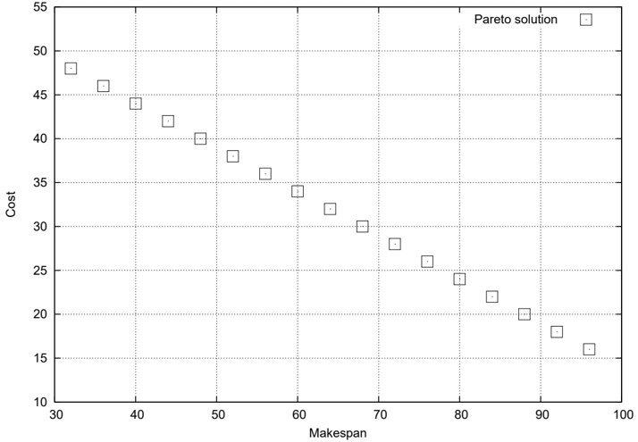
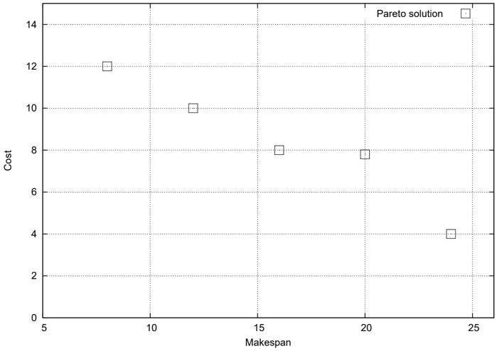
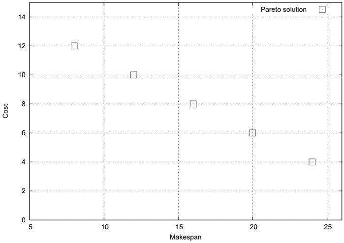
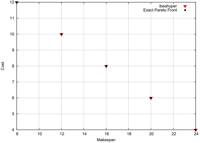
In both cases, there are 3 obvious points that belong to the Pareto Front: the solution with minimal makespan described above, and the similar solutions that use respectively city 2 and city 3 in lieu of city 1 . The values of the makespans are respectively 8, 16 and 24, and the values of the costs are, for each solution, 4 times the value of the single landing tax, and exactly the value of the involved risk. For the risk case, there is no other point on the Pareto Front, as a single landing on a high-risk city sets the risk of the whole plan to a high risk. For the cost model however, there are other points on the Pareto Front, as different cities can be used for the different passengers. For instance, in the case of Figure 1, this leads to a Pareto Front made of 5 points, (8,12), (16,8), and (24,4) (going only through city 1 , 2 and 3 respectively), plus (12,10) and (20,6). Only the first 3 are the Pareto Front in the risk case.

4.1 Tuning the Complexity

There are several ways to make this first simple instance more or less complex. A first possibility is to add passengers. In this work, only bunches of 3 passengers have been considered, in order to be able to easily derive some obvious Pareto-optimal solutions, using several times the little trick to avoid leaving any plane idle. For instance, it is easy to derive all the Pareto solutions for 6 and 9 passengers - and in the following, the corresponding instances will be termed MultiZeno 3, MultiZeno 6, and MultiZeno 9 respectively (sub-scripted with the type of second objective - cost or risk).

Of course, the number of planes could also be increased, though the number of passengers needs to remain larger than the number of planes to allow for nontrivial Pareto front. However, departing from the 3 passengers to 2 planes ratio would make the Pareto front not easy to identify any more.

Another possibility is to increase the number of central cities: this creates more points on the Pareto front, using either plans in which a single city is used for all passengers, or plans that use several different cities for different passengers (while nevertheless using the same trick to ensure no plane stays idle). In such configuration too the exact Pareto front remains easy to identify: further work will investigate this line of complexification.

4.2 Modifying the shape of the Pareto Front

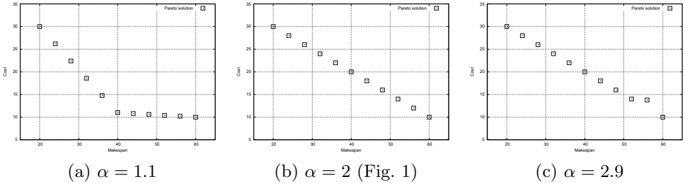
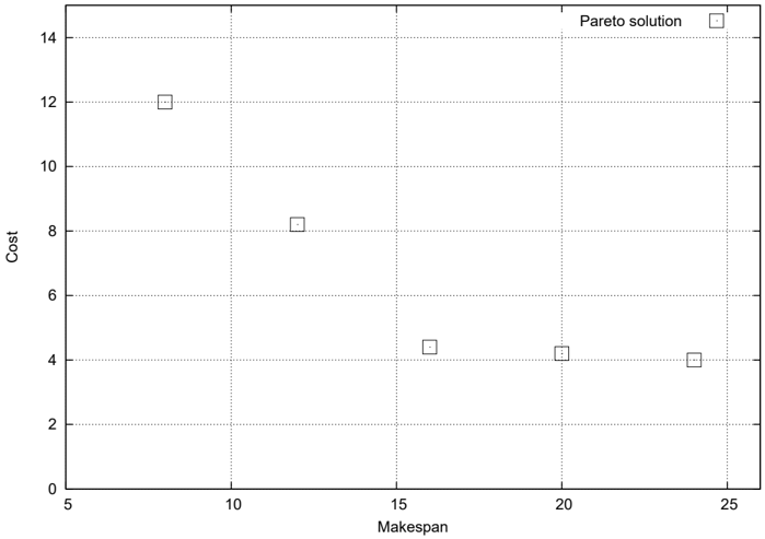
Another way to change the difficulty of the problem without increasing its complexity is to tune the different values of the flight times and the cost/risk at each city. Such changes does not modify the number of points on the Pareto Front, but does change its shape in the objective space. For instance, simply modifying the cost α of city2 , the central city in Figure 1, between 1 and 3 (the costs of respectively city1 and city3 ), the Pareto Front, which is linear for α = 2 becomes strictly convex for α < 2 and strictly concave for α > 2, as can be seen for two extreme cases ( α = 1 . 1 and α = 2 . 9) on Figure 2. Further work will address the identification of the correct domain parameters in order to reach a given shape of the Pareto front.

5 Experimental Conditions

Implementation: All proposed multi-objective approaches (see Section 3.2) have been implemented within the ParadisEO-MOEO framework [18]. All experiments were performed on the MultiZeno 3, MultiZeno 6, and MultiZeno 9 instances. The first objective is the makespan, and the second objective either the (additive) cost or the (maximal) risk, as discussed in Section 4. The values of the different flight durations and cost/risks are those given on Figure 1 except otherwise stated.

Parameter tuning: All user-defined parameters have been tuned using the framework ParamILS [19]. ParamILS handles any parameterized algorithm whose parameters can be discretized. Based on Iterated Local Search (ILS), ParamILS searches through the space of possible parameter configurations, evaluating configurations by running the algorithm to be optimized on a set of benchmark instances, searching for the configuration that yields overall best performance across the benchmark problems. Here, both the parameters of the multi-objective algorithms (including the internal parameters of the variation operators - see [20]) and YAHSP specific parameters (including the relative weights of the possible strategies (see Section 3.1) have been subject to ParamILS optimization.

For the purpose of this work, parameters were tuned anew for each instance (see [20] for a discussion about the generality of such parameter tuning, that falls beyond the scope of this paper).

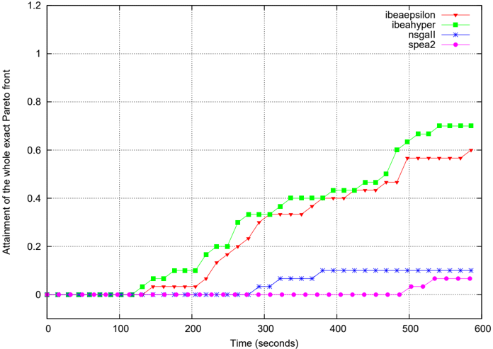
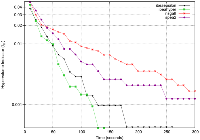
Performance Metric: The quality measure used by ParamILS to optimize DaEYAHSP is the unary hypervolume I H -[16] of the set of non-dominated points output by the algorithm with respect to the complete true Pareto front (only instances where the true Pareto front is fully known have been experimented with). The lower the better (a value of 0 indicates that the exact Pareto front has been reached).

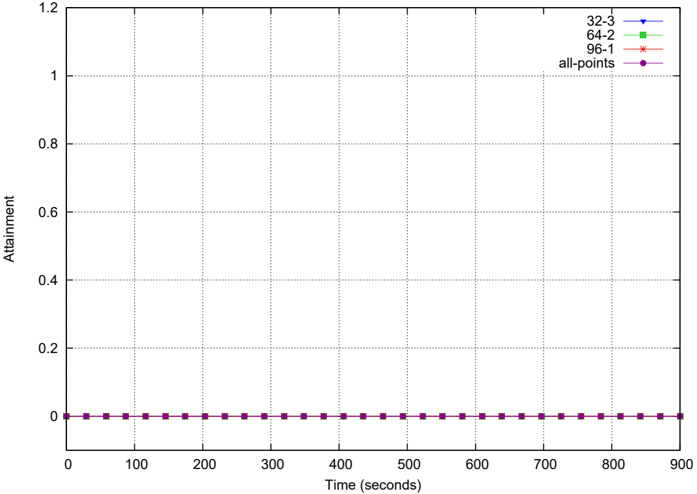
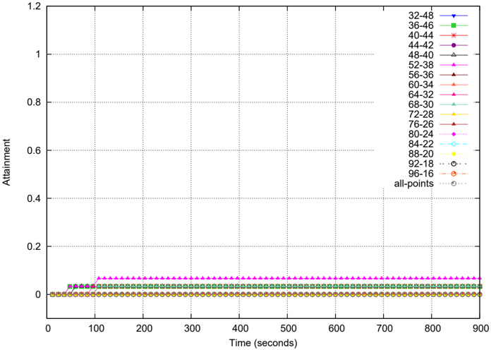
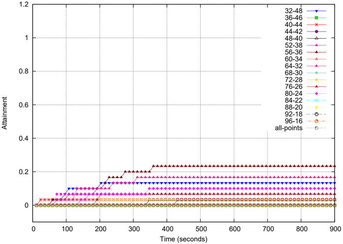
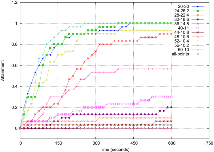
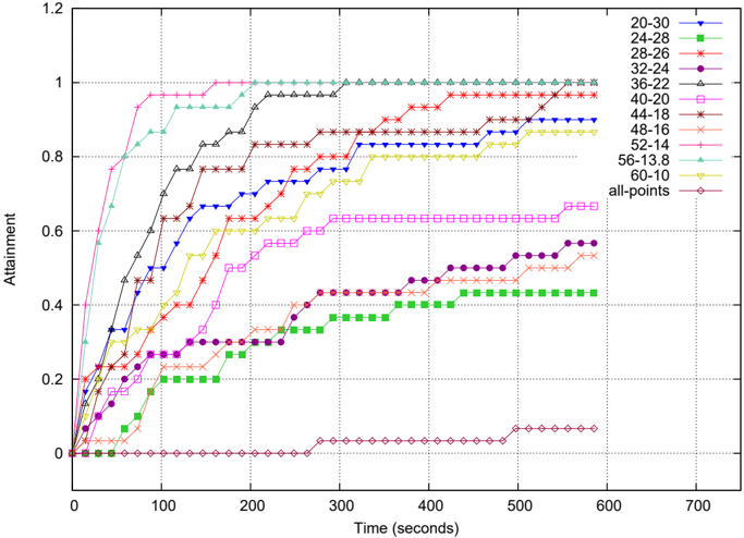
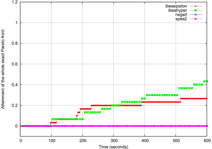
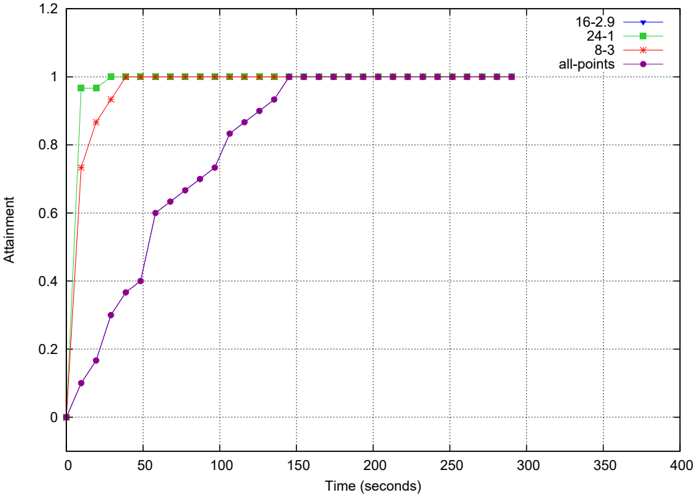
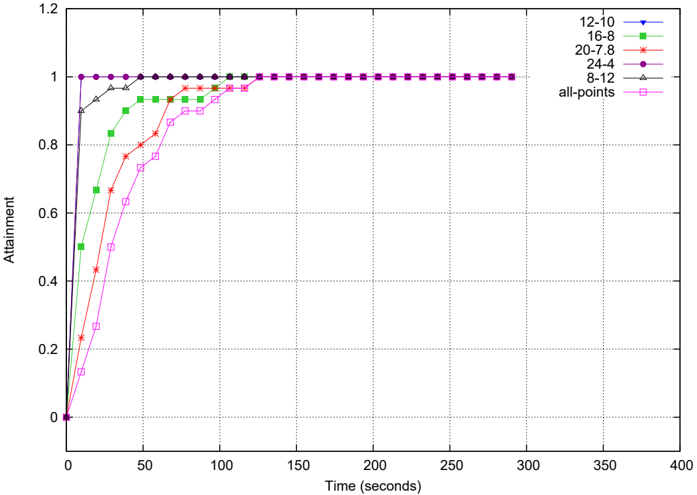
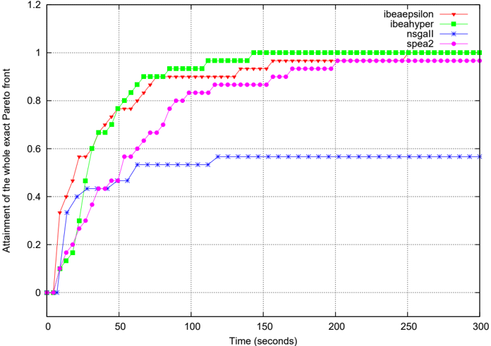
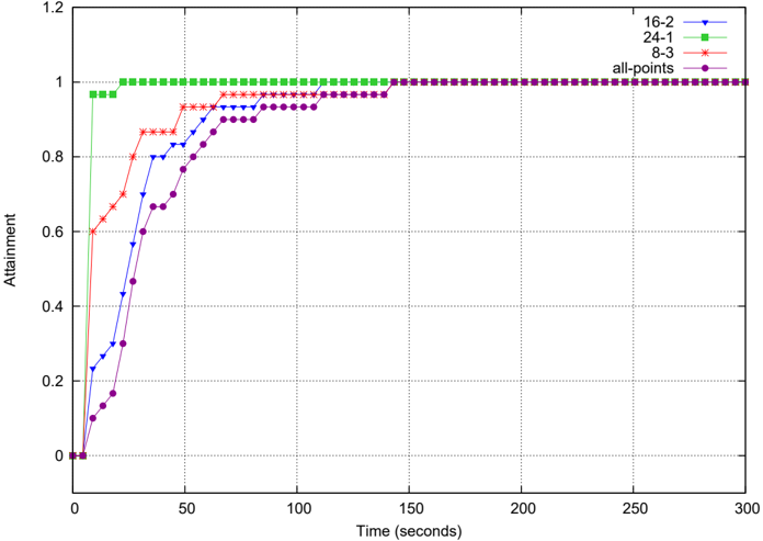
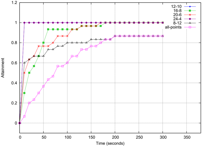
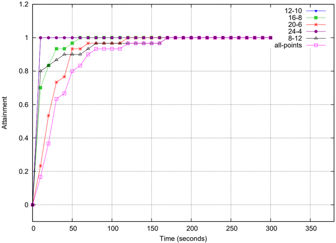
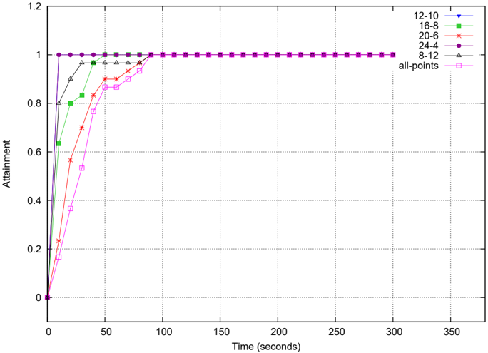
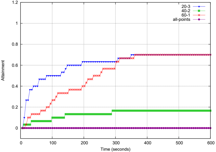
However, and because the true front is known exactly, and is made of a few scattered points (at most 17 for MultiZeno 9 in this paper), it is also possible to visually monitor when each point of the front is discovered by the algorithm. This allows some deeper comparison between algorithms even when none has found the whole front. Such attainment plots will be used in the following, together with more classical plots of hypervolume vs time.

For all experiments, 30 independent runs were performed. Note that all the performance assessment procedures, including the hypervolume calculations, have been achieved using the PISA performance assessment tool suite [21].

Stopping Criterion: Because different fitness evaluations involve different number calls to YAHSP - and because YAHSP runs can have different computational costs too, depending on the difficulty of the sub-problem being solved the stopping criterion was a fixed amount of CPU time rather than the usual number of fitness evaluation. These absolute limits were set to 300, 600, and 900 seconds respectively for MultiZeno 3, MultiZeno 6, and MultiZeno 9.

6 Experimental Results

6.1 Comparing Multi-Objective Schemes

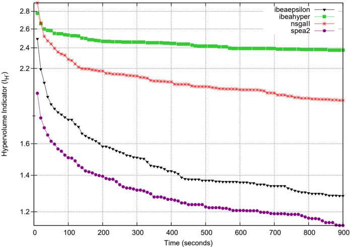
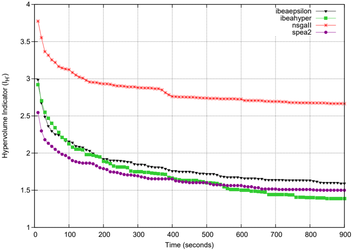
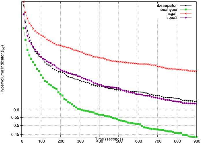
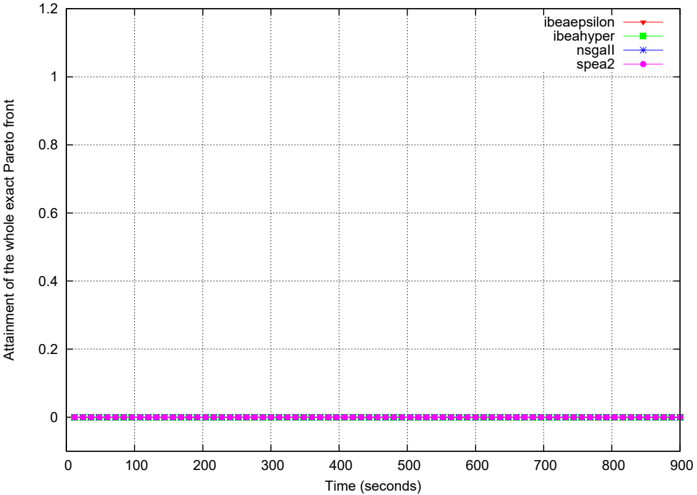
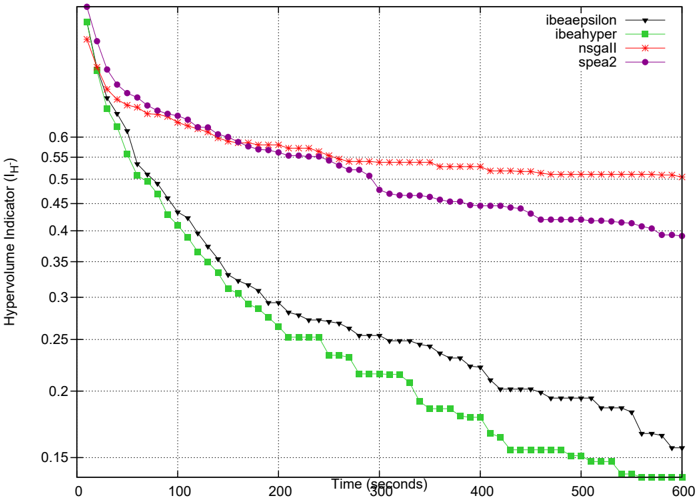
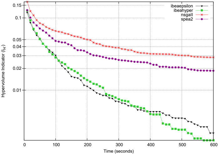
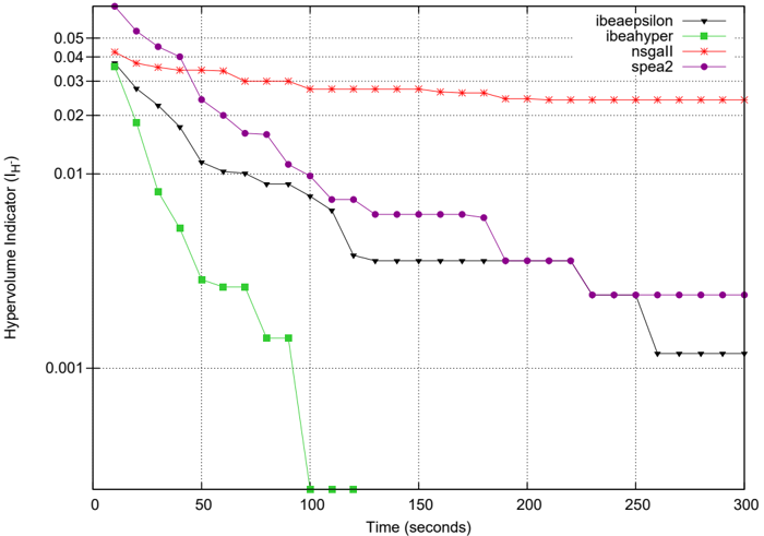
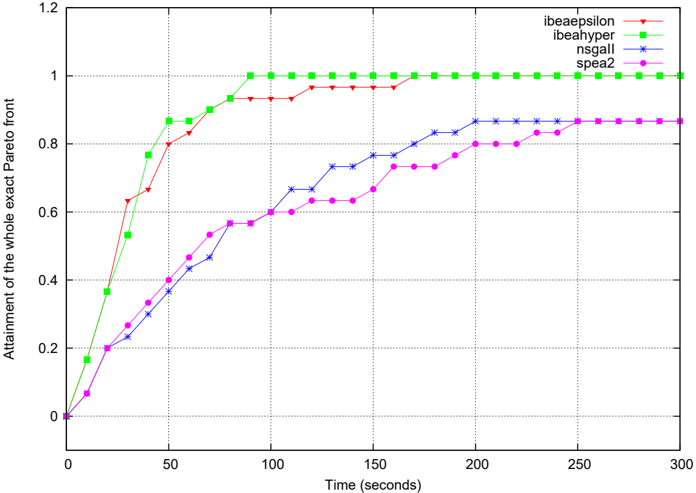
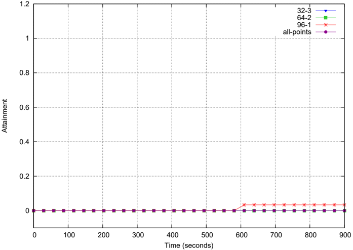
The first series of experiments presented here are concerned with the comparison of the different multi-objective schemes briefly introduced in Section 3.2. Figure 3 displays a summary of experiments of all 4 variants for MultiZeno instances for both the Cost and Risk problems.

Some clear conclusions can be drawn from these results, that are confirmed by the statistical analyses presented in Table 1 using Wilcoxon signed rank test with 95% confidence level. First, looking at the minimal values of the hypervolume reached by the different algorithms shows that, as expected, the difficulty of the problems increases with the number of passengers, and for a given complexity, the Risk problems are more difficult to solve than the Cost ones. Second, from the plots and the statistical tests, it can be seen that NSGA-II is outperformed by all other variants on all problems, SPEA2 by both indicator-based variants on most instances, and IBEA H -is a clear winner over IBEA ε + except on MultiZeno 6 risk .

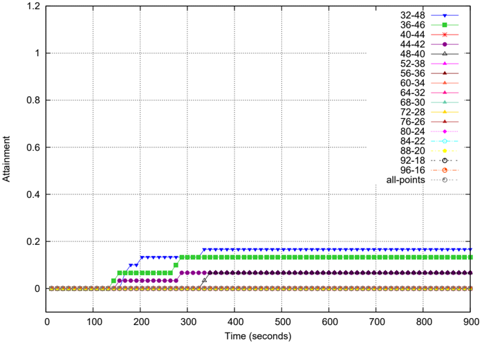
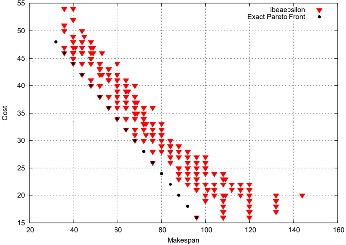
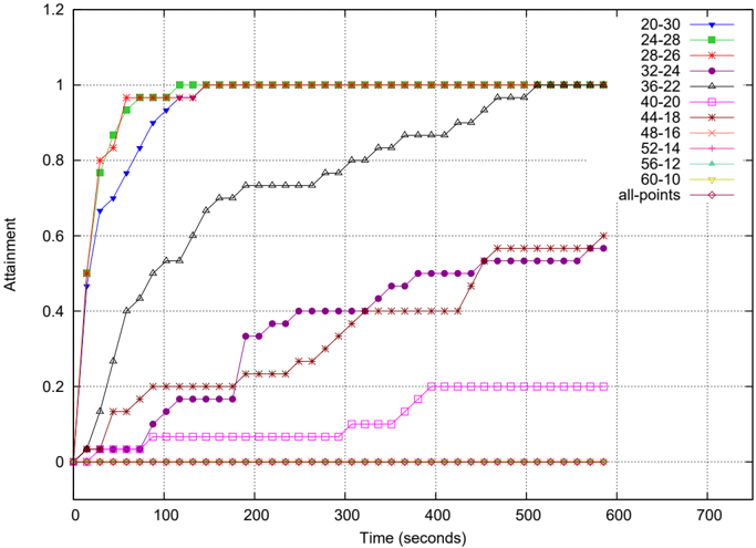
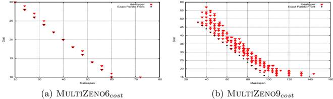
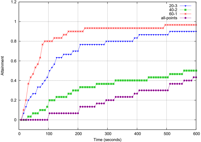
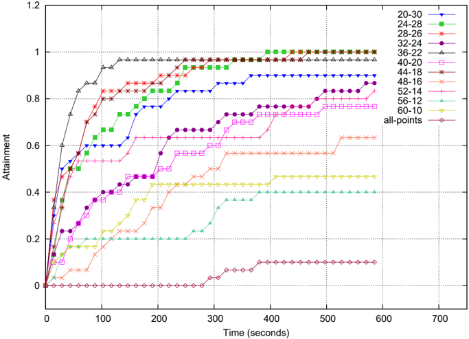
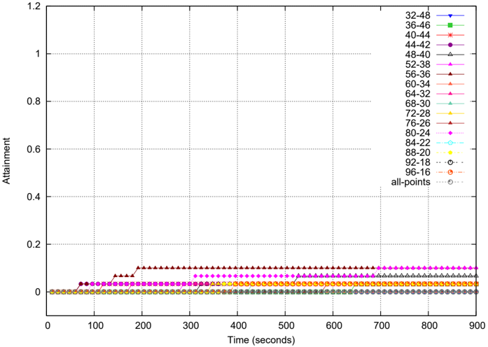
More precisely, Figure 4 show the cumulated final populations of all 30 runs in the objective space together with the true Pareto front for MultiZeno 6- 9 cost problems: the situation is not as bad as it seemed from Figure 3-(e) for MultiZeno 9 cost , as most solutions that are returned by IBEA H - are close to the Pareto front (this is even more true on MultiZeno 6 cost problem). A dynamic view of the attainment plots is given in Figure 6-(c): two points of the Pareto front are more difficult to reach than the others, namely (48,16) and (56,12).

• (a) MultiZeno 3 cost

• (b) MultiZeno 3 risk

• (c) MultiZeno 6 cost

• (d) MultiZeno 6 risk

• (e) MultiZeno 9 cost

• (f) MultiZeno 9 risk

Fig. 3: Evolution of the Hypervolume indicator I H -(averaged over 30 runs) on MultiZeno instances (see Table 1 for statistical significances).

• (a) MultiZeno 6 cost
• (b) MultiZeno 6 risk

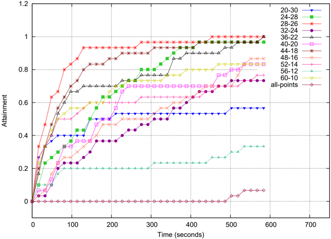
Fig. 5: Attainment plots for IBEA H -on MultiZeno 6 instances.

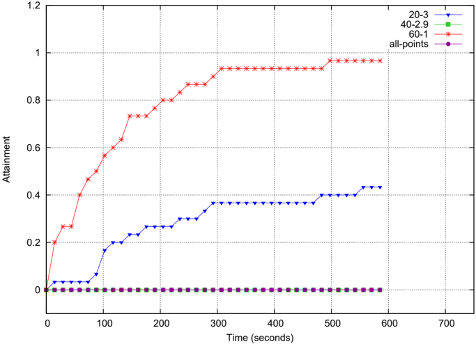
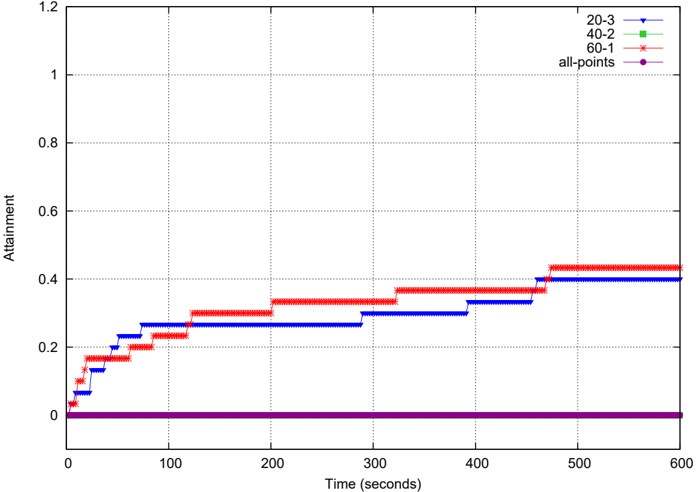
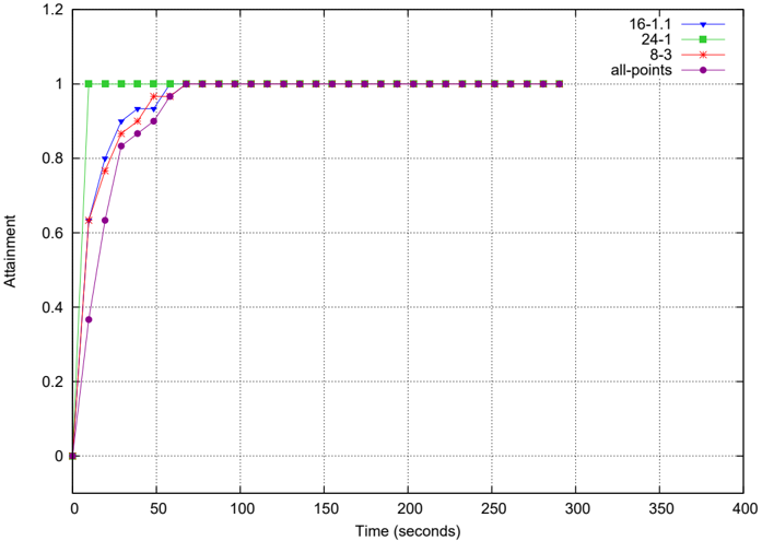
6.2 Influence of YAHSP Strategy

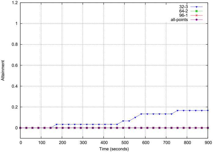
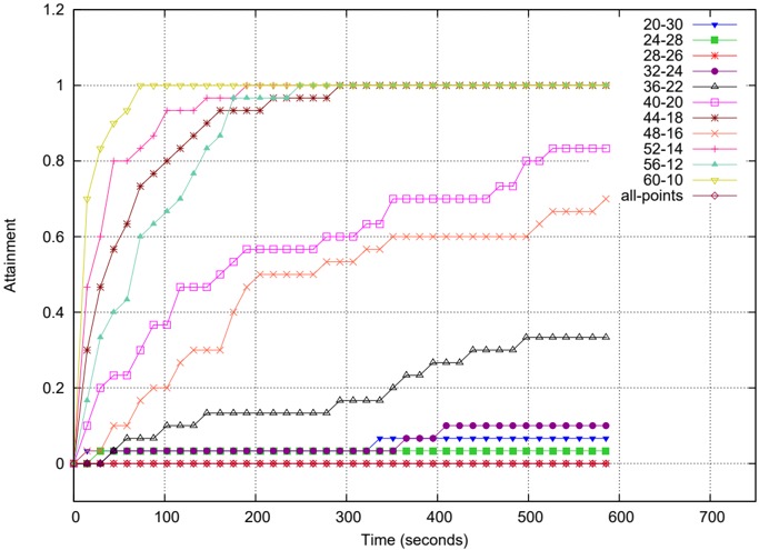
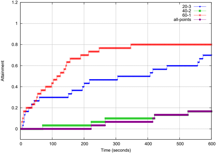
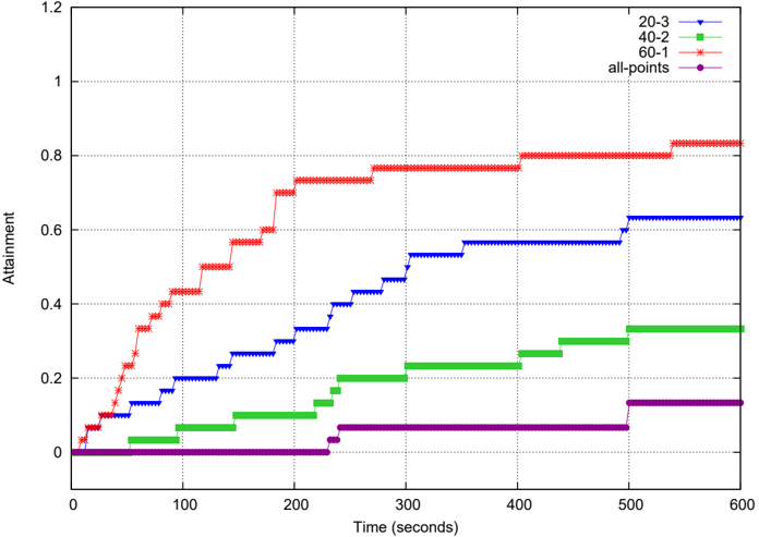
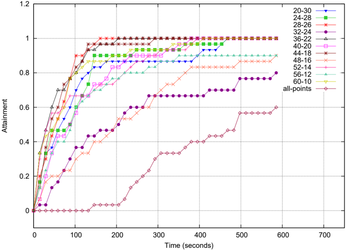
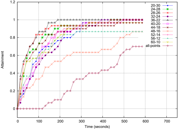
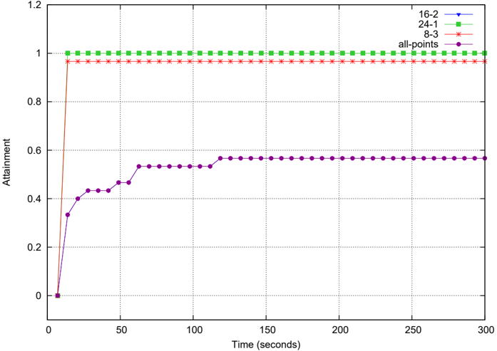
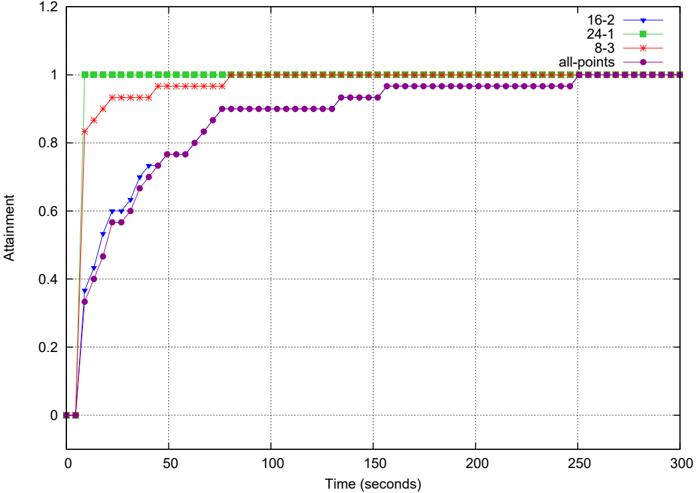
Next series of experiments aimed at identifying the influence of the chosen strategy for YAHSP (see Section 3.1). Figure 6-(a) (resp. 6-(b)) shows the attainment plots for the strategy in which YAHSP always optimizes the makespan (resp. the cost) on problem MultiZeno 6 cost . Both extreme strategies lead to much worse results than the mixed strategy of Figure 5-(a), as no run discovers the whole front (last line, that never leaves the x-axis). Furthermore, and as could be expected, the makespan-only strategy discovers very rapidly the extreme points of the Pareto front that have a small makespan (points (20,30), (24,28) and (28,26)) and hardly discovers the other end of the Pareto front (points with makespan greater than 48), while it is exactly the opposite for the cost-only strategy. This confirms the need for a strategy that incorporates both approaches. best possible choice.

Note that similar conclusion could have been drawn from ParamILS results on parameter tuning (see Section 5): the choice of YAHSP strategy was one of the parameters tuned by ParamILS . . . and the tuned values for the weights of both strategies were always more or less equal.

Table 1: Wilcoxon signed rank tests at 95% confidence level (I H -metric).

Instances	Algorithms	Algorithms
		NSGAII	IBEA ε +	IBEA H -	SPEA 2
Zeno3 cost	NSGAII	-	≡	≡	≡
	IBEA ε +	≡	-	≡	≡
	IBEA H -	≡	≡	-	≡
	SPEA 2	≡	≡	≡	-
Zeno3 risk	NSGAII	-	≡	≡	≡
	IBEA ε +	≡	-	≡	/follows
	IBEA H -	≡	≡	-	/follows
	SPEA 2	≡	≺	≺	-
Zeno6 cost	NSGAII	-	≺	≺	≺
	IBEA ε +	/follows	-	≡	≡
	IBEA H -	/follows	≡	-	≡
	SPEA 2	/follows	≡	≡	-
Zeno6 risk	NSGAII	-	≺	≺	≡
	IBEA ε +	/follows	-	/follows	/follows
	IBEA H -	/follows	≺	-	/follows
	SPEA 2	≡	≺	≺	-
Zeno9 cost	NSGAII	-	≺	≺	≺
	IBEA ε +	/follows	-	≺	≡
	IBEA H -	/follows	/follows	-	≡
	SPEA 2	/follows	≡	≡	-
Zeno9 risk	NSGAII	-	≺	≺	≺
	IBEA ε +	/follows	-	≺	≡
	IBEA H -	/follows	/follows	-	≡
	SPEA 2	/follows	≡	≡	-

• (a) YAHSP optimizes makespan
• (b) YAHSP optimizes cost

Fig. 6: Attainment plots for two search strategies on MultiZeno 6 cost .

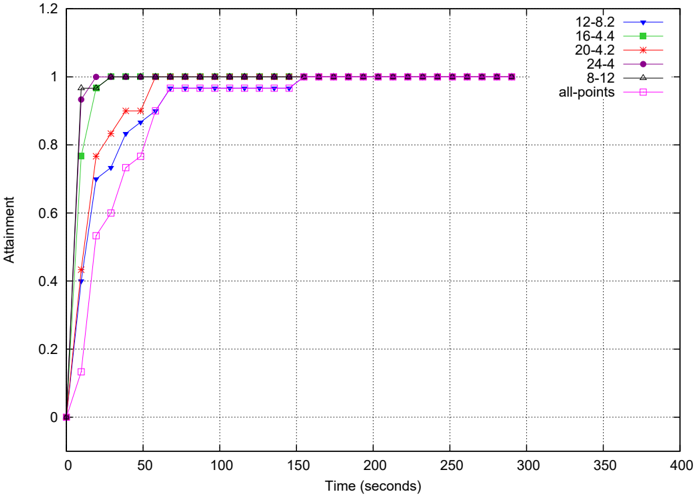
6.3 Shape of the Pareto Front

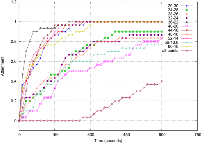
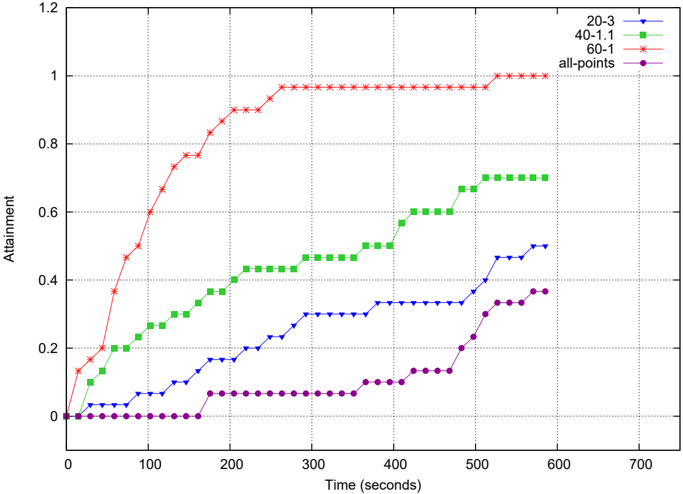
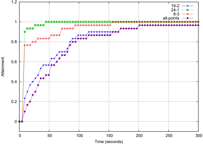
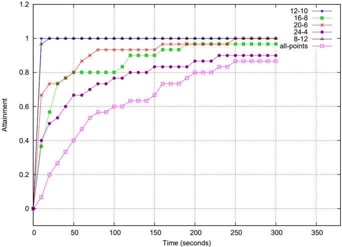
Figure 7 displays the attainment plots of IBEA H -for both extreme Pareto fronts shown on Figure 2 - while the corresponding plot for the linear case α = 2 is that of Figure 5-(a). Whereas the concave front is fully identified in 40% of the runs (right), the complete front for the strictly convex case (left) is never reached: in the latter case, the 4 most extreme points are found by 90% of the runs in less than 200 seconds, while the central points are hardly ever found. We hypothesize that the handling of YAHSP strategy regarding which objective to optimize (see Section 3.1) has a greater influence in the case of this strictly

Fig. 7: Attainment plots for different Pareto fronts for MultiZeno 6 cost .

convex front than when the front is linear ( α = 2) or almost linear, even if strictly concave ( α = 2 . 9). In any case, no aggregation technique could ever solve the latter case, whereas it is here solved in 40% of the runs by DaEYAHSP .

7 Conclusion and Perspectives

The contributions of this paper are twofold. Firstly, MultiZeno , an original benchmark test suite for multi-objective temporal planning, has been detailed, and several levers identified that allow to generate more or less complex instances, that have been confirmed experimentally: increasing the number of passengers obviously makes the problem more difficult; modifying the cost of reaching the cities and the duration of the flights is another way to make the problem harder, though deeper work is required to identify the consequences of each modification. Secondly, several multi-objectivization of DaEX , an efficient evolutionary planner in the single-objective case, have been proposed.

However, even though the hypervolume-based IBEA H -clearly emerged as the best choice, the experimental comparison of those variants on the MultiZeno benchmark raises more questions than it brings answers. The sparseness of the Pareto Front has been identified as a possible source for the rather poor performance of all variants for moderately large instances, particularly for the risk type of instances. Some smoothening of the objectives could be beneficial to tackle this issue (e.g., counting for the number of times each risk level is hit rather than simply accounting for the maximal value reached). Another direction of research is to combat the non-symmetry of the results, due to the fact that the embedded planner only optimizes one objective. Further work will investigate a self-adaptive approach to the choice of which objective to give YAHSP to optimize. Finally, the validation of the proposed multi-objective DaEYAHSP can only be complete after a thorough comparison with the existing aggregation approaches - though it is clear that aggregation approaches will not be able to identify the whole Pareto front in case it has some concave parts, whereas the results reported here show that DaEYAHSP can reasonably do it.

References

1. Ghallab, M., Nau, D., Traverso, P.: Automated Planning, Theory and Practice. Morgan Kaufmann (2004)
2. Do, M., Kambhampati, S.: SAPA: A Multi-Objective Metric Temporal Planner. J. Artif. Intell. Res. (JAIR) 20 (2003) 155-194
3. Refanidis, I., Vlahavas, I.: Multiobjective Heuristic State-Space Planning. Artificial Intelligence 145 (1) (2003) 1-32
4. Gerevini, A., Saetti, A., Serina, I.: An Approach to Efficient Planning with Numerical Fluents and Multi-Criteria Plan Quality. Artificial Intelligence 172(8-9) (2008) 899-944
5. Chen, Y., Wah, B., Hsu, C.: Temporal Planning using Subgoal Partitioning and Resolution in SGPlan. J. of Artificial Intelligence Research 26 (1) (2006) 323-369
6. Edelkamp, S., Kissmann, P.: Optimal Symbolic Planning with Action Costs and Preferences. In: Proc. 21 st IJCAI. (2009) 1690-1695
7. Schoenauer, M., Sav´ eant, P., Vidal, V.: Divide-and-Evolve: a New Memetic Scheme for Domain-Independent Temporal Planning. In Gottlieb, J., Raidl, G., eds.: Proc. 6 th EvoCOP, LNCS 3906, Springer (2006) 247-260
8. Vidal, V.: A Lookahead Strategy for Heuristic Search Planning. In: Proceedings of the 14 th ICAPS, AAAI Press (2004) 150-159
9. Fikes, R., Nilsson, N.: STRIPS: A New Approach to the Application of Theorem Proving to Problem Solving. Artificial Intelligence 1 (1971) 27-120
10. Biba¨ ı, J., Sav´ eant, P., Schoenauer, M., Vidal, V.: An Evolutionary Metaheuristic Based on State Decomposition for Domain-Independent Satisficing Planning. In R. Brafman et al., ed.: Proc. 20 th ICAPS, AAAI Press (2010) 18-25
11. Biba¨ ı, J., Sav´ eant, P., Schoenauer, M., Vidal, V.: On the Benefit of Sub-Optimality within the Divide-and-Evolve Scheme. In Cowling, P., Merz, P., eds.: Proc. 10 th EvoCOP, LNCS 6022, Springer Verlag (2010) 23-34
12. Haslum, P., Geffner, H.: Admissible Heuristics for Optimal Planning. In: Proc. AIPS-2000. (2000) 70-82
13. Gerevini, A., Long, D.: Preferences and Soft Constraints in PDDL3. In: ICAPS Workshop on Planning with Preferences and Soft Constraints. (2006) 46-53
14. Deb, K., Pratap, A., Agarwal, S., Meyarivan, T.: A fast and elitist multiobjective genetic algorithm: NSGA-II. IEEE Trans. Evol. Comp. 6 (2) (2002) 182-197
15. Zitzler, E., Laumanns, M., Thiele, L.: SPEA2: Improving the Strength Pareto Evolutionary Algorithm for Multiobjective Optimization. In: Evol. Methods Design Optim. Control Applicat. Ind. Prob. (EUROGEN). (2002) 95-100
16. Zitzler, E., K¨ unzli, S.: Indicator-Based Selection in Multiobjective Search. In Xin Yao et al., ed.: Proc. PPSN VIII, LNCS 3242, Springer Verlag (2004) 832-842
17. Zitzler, E., Laumanns, M., Thiele, L.: SPEA2: Improving the Strength Pareto Evolutionary Algorithm. Technical report, ETH Z¨ urich (2001)
18. Liefooghe, A., Basseur, M., Jourdan, L., Talbi, E.: ParadisEO-MOEO: A framework for evolutionary multi-objective optimization. In: Evolutionary multicriterion optimization, Springer (2007) 386-400
19. Hutter, F., Hoos, H.H., Leyton-Brown, K., St¨ utzle, T.: ParamILS: an automatic algorithm configuration framework. J. Artif. Intell. Res. (JAIR) 36 (2009) 267-306
20. Biba¨ ı, J., Sav´ eant, P., Schoenauer, M., Vidal, V.: On the Generality of Parameter Tuning in Evolutionary Planning. In: Proc 12 th GECCO, ACM (2010) 241-248
21. Bleuler, S., Laumanns, M., Thiele, L., Zitzler, E.: PISA a platform and programming language independent interface for search algorithms. In: Evolutionary Multi-Criterion Optimization. Volume 2632 of LNCS. Springer (2003) 494-508

Instructions for Authors Coding with L A T E X

L A T E X 2 ε Class for Lecture Notes in Computer Science

Version 2.4

• 2 L A T E X 2 ε Class for Lecture Notes in Computer Science

For further information please contact us:

• LNCS Editorial Office

Springer-Verlag Computer Science Editorial Tiergartenstrae 17 69121 Heidelberg Germany
Tel: Fax: e-mail:	+49-6221-487-8706 +49-6221-487-8588	for editorial questions for T E X problems
We are	also reachable through http://www.springer.com http://www.springer.com/lncs http://www.springerlink.com ftp://ftp.springer.de	the world wide web: Springer Global Website LNCS home page data repository FTP server

Table of Contents

1	Introduction. . . . . . . . . . . . . . . . . . . . . . . . . . . . . . . . . . . . . . . . . . .		. . . . . .	4
2	How to Proceed. .		. . . . . . . . . . . . . . . . . . . . . . . . . . . . . . . . . . . . . . . . . . . .	4
	2.1	How to Invoke the LLNCS Document Class . . . . . . . . . . .	4
	2.2	. . . . . . Contributions Already Coded with L A T E X without the LLNCS document class . . . . . . . . . . . . . . . . . . . . . . . . . . . . . . . . . . . . . . . . . .	5
3	General Rules for Coding Formulas. . . . . . . . .		. . . . . . . . . . . . . . . . . . . .	5
	3.1	Italic and Roman Type in Math Mode . . . . . . . . . . . . . . . . . . . . .	6
4	How	to Edit Your Input (Source) File . . . . . . . . . . . . . . . . . . . . . . . . . .	6
	4.1	Headings . . . . . . . . . . . . . . . . . . . . . . . . . . . . . . . . . . . . . . . . . . . . . . .	6
	4.2	Capitalization and Non-capitalization . . . . . . . . . . . . . . . . . . . . . .	6
	4.3	Abbreviation of Words . . . . . . . . . . . . . . . . . . . . . . . . . . . . . . . . . . .	7
5	How to Code the Beginning of Your Contribution .		. . . . . . . . . . . . . . .	7
6	Special Commands for the Volume Editor .		. . . . . . . . . . . . . . . . . . . . . .	9
7	How to Code Your Text . .		. . . . . . . . . . . . . . . . . . . . . . . . . . . . . . . . . . . .	10
8	Predefined Theorem like Environments .		. . . . . . . . . . . . . . . . . . . . . . . .	10
9	Defining your Own Theorem like Environments . . . . .		. . . . . . . . . . . . .	11
	9.1	Method 1 (preferred) . . . . . . . . . . . . . . . . . . . . . . . . . . . . . . . . . . . . .	11
	9.2	Method 2 . . . . . . . . . . . . . . . . . . . . . . . . . . . . . . . . . . . . . . . . . . . . . .	12
	9.3	Unnumbered Environments . . . . . . . . . . . . . . . . . . . . . . . . . . . . . . .	12
10	Program Codes . . . .		. . . . . . . . . . . . . . . . . . . . . . . . . . . . . . . . . . . . . . . . . .	12
11	Fine Tuning of the Text . .		. . . . . . . . . . . . . . . . . . . . . . . . . . . . . . . . . . . .	16
12	Special Typefaces . . .		. . . . . . . . . . . . . . . . . . . . . . . . . . . . . . . . . . . . . . . . .	16
13	Footnotes . . . . . . . . . . .		. . . . . . . . . . . . . . . . . . . . . . . . . . . . . . . . . . . . . . . .	17
14	Lists . .		. . . . . . . . . . . . . . . . . . . . . . . . . . . . . . . . . . . . . . . . . . . . . . . . . . . . .	17
15		Figures . . . . . . . . . . . . . . . . . . . . . . . . . . . . . . . . . . . . . . . . . . . . . . . . . . . . .	17
16		Tables . . . . . . . . . . . . . . . . . . . . . . . . . . . . . . . . . . . . . . . . . . . . . . . . . . . . . .	18
	16.1 Tables Coded with L A T E X. .		. . . . . . . . . . . . . . . . . . . . . . . . . . . . . . .	19
	16.2 Tables Not Coded with L A T E X.		. . . . . . . . . . . . . . . . . . . . . . . . . . . .	19
	16.3 Signs and Characters		. . . . . . . . . . . . . . . . . . . . . . . . . . . . . . . . . . . .	20
17	References		. . . . . . . . . . . . . . . . . . . . . . . . . . . . . . . . . . . . . . . . . . . . . . . . . .	21
	17.1 References by Letter-Number or by Number Only . . . .		. . . . . . .	21
	17.2 Author-Year System . . . .		. . . . . . . . . . . . . . . . . . . . . . . . . . . . . . . . .	22

1 Introduction

Authors wishing to code their contribution with L A T E X, as well as those who have already coded with L A T E X, will be provided with a document class that will give the text the desired layout. Authors are requested to adhere strictly to these instructions; the class file must not be changed .

The text output area is automatically set within an area of 12.2 cm horizontally and 19.3 cm vertically.

If you are already familiar with L A T E X, then the LLNCS class should not give you any major difficulties. It will change the layout to the required LLNCS style (it will for instance define the layout of \section ). We had to invent some extra commands, which are not provided by L A T E X (e.g. \institute , see also Sect. 5)

For the main body of the paper (the text) you should use the commands of the standard L A T E X 'article' class. Even if you are familiar with those commands, we urge you to read this entire documentation thoroughly. It contains many suggestions on how to use our commands properly; thus your paper will be formatted exactly to LLNCS standard. For the input of the references at the end of your contribution, please follow our instructions given in Sect. 17 References.

The majority of these hints are not specific for LLNCS; they may improve your use of L A T E X in general. Furthermore, the documentation provides suggestions about the proper editing and use of the input files (capitalization, abbreviation etc.) (see Sect. 4 How to Edit Your Input File).

2 How to Proceed

The package consists of the following files:

history.txt	the version history of the package
llncs.cls	class file for L A T E X
llncs.dem	an example showing how to code the text
llncs.doc	general instructions (source of this document), llncs.doc means l atex doc umentation for
llncsdoc.pdf	the documentation of the class (PDF version),
llncs.doc	general instructions (source of this document),
llncsdoc.sty	class modifications to help for the instructions
llncs.ind subjidx.ind	an external (faked) author index file subject index demo from the Springer book package
llncs.dvi	the resultig DVI file (remember to use binary transfer!)
sprmindx.sty	supplementary style file for MakeIndex (usage: makeindex -s sprmindx.sty <yourfile.idx>

2.1 How to Invoke the LLNCS Document Class

The LLNCS class is an extension of the standard L A T E X 'article' document class. Therefore you may use all 'article' commands for the body of your contribution

to prepare your manuscript. LLNCS class is invoked by replacing 'article' by 'llncs' in the first line of your document:

\documentclass{llncs} % \begin{document}

2.2 Contributions Already Coded with L A T E X without the LLNCS document class

If your file is already coded with L A T E X you can easily adapt it a posteriori to the LLNCS document class.

Please refrain from using any L A T E X or T E X commands that affect the layout or formatting of your document (i.e. commands like \textheight , \vspace , \headsep etc.). There may nevertheless be exceptional occasions on which to use some of them.

The LLNCS document class has been carefully designed to produce the right layout from your L A T E X input. If there is anything specific you would like to do and for which the style file does not provide a command, please contact us . Same holds for any error and bug you discover (there is however no reward for this sorry).

3 General Rules for Coding Formulas

With mathematical formulas you may proceed as described in Sect. 3.3 of the L A T E X User's Guide & Reference Manual by Leslie Lamport (2nd ed. 1994), Addison-Wesley Publishing Company, Inc.

Equations are automatically numbered sequentially throughout your contribution using arabic numerals in parentheses on the right-hand side.

When you are working in math mode everything is typeset in italics. Sometimes you need to insert non-mathematical elements (e.g. words or phrases). Such insertions should be coded in roman (with \mbox ) as illustrated in the following example:

Sample Input

\begin{equation} \left(\frac{a^{2} + b^{2}}{c^{3}} \right) = 1 \quad \mbox{ if } c\neq 0 \mbox{ and if } a,b,c\in \bbbr \enspace . \end{equation}

Sample Output

/negationslash

If you wish to start a new paragraph immediately after a displayed equation, insert a blank line so as to produce the required indentation. If there is no new paragraph either do not insert a blank line or code \noindent immediately before continuing the text.

Please punctuate a displayed equation in the same way as other ordinary text but with an \enspace before end punctuation.

Note that the sizes of the parentheses or other delimiter symbols used in equations should ideally match the height of the formulas being enclosed. This is automatically taken care of by the following L A T E X commands:

\left( or \left[ and \right) or \right] .

3.1 Italic and Roman Type in Math Mode

1. In math mode L A T E X treats all letters as though they were mathematical or physical variables, hence they are typeset as characters of their own in italics. However, for certain components of formulas, like short texts, this would be incorrect and therefore coding in roman is required. Roman should also be used for subscripts and superscripts in formulas where these are merely labels and not in themselves variables, e.g. T eff not T eff , T K not T K (K = Kelvin), m e not m e (e = electron). However, do not code for roman if the sub/superscripts represent variables, e.g. n i =1 a i .
2. ∑ b) Please ensure that physical units (e.g. pc, erg s -1 K, cm -3 , W m -2 Hz -1 , m kg s -2 A -2 ) and abbreviations such as Ord, Var, GL, SL, sgn, const. are always set in roman type. To ensure this use the \mathrm command: \mathrm{Hz} . On p. 44 of the L A T E X User's Guide & Reference Manual by Leslie Lamport you will find the names of common mathematical functions, such as log, sin, exp, max and sup. These should be coded as \log , \sin , \exp , \max , \sup and will appear in roman automatically.
3. Chemical symbols and formulas should be coded for roman, e.g. Fe not Fe , H 2 O not H 2 O .
4. Familiar foreign words and phrases, e.g. et al., a priori, in situ, bremsstrahlung, eigenvalues should not be italicized.

4 How to Edit Your Input (Source) File

4.1 Headings

All words in headings should be capitalized except for conjunctions, prepositions (e.g. on, of, by, and, or, but, from, with, without, under) and definite and indefinite articles (the, a, an) unless they appear at the beginning. Formula letters must be typeset as in the text.

4.2 Capitalization and Non-capitalization

1. The following should always be capitalized:

• Headings (see preceding Sect. 4.1)
• Abbreviations and expressions in the text such as Fig(s)., Table(s), Sect(s)., Chap(s)., Theorem, Corollary, Definition etc. when used with numbers, e.g. Fig. 3, Table 1, Theorem 2.

Please follow the special rules in Sect. 4.3 for referring to equations.

1. The following should not be capitalized:
2. The words figure(s), table(s), equation(s), theorem(s) in the text when used without an accompanying number.
3. Figure legends and table captions except for names and abbreviations.

4.3 Abbreviation of Words

1. The following should be abbreviated when they appear in running text unless they come at the beginning of a sentence: Chap., Sect., Fig.; e.g. The results are depicted in Fig. 5. Figure 9 reveals that . . . .
2. Please note : Equations should usually be referred to solely by their number in parentheses: e.g. (14). However, when the reference comes at the beginning of a sentence, the unabbreviated word 'Equation' should be used: e.g. Equation (14) is very important. However, (15) makes it clear that . . . .
3. If abbreviations of names or concepts are used throughout the text, they should be defined at first occurrence, e.g. Plurisubharmonic (PSH) Functions, Strong Optimization (SOPT) Problem.

5 How to Code the Beginning of Your Contribution

The title of a single contribution (it is mandatory) should be coded as follows:

\title{

All words in titles should be capitalized except for conjunctions, prepositions (e.g. on, of, by, and, or, but, from, with, without, under) and definite and indefinite articles (the, a, an) unless they appear at the beginning. Formula letters must be typeset as in the text. Titles have no end punctuation.

If a long \title must be divided please use the code \\ (for new line).

If you are to produce running heads for a specific volume the standard (of no such running heads) is overwritten with the [runningheads] option in the \documentclass line. For long titles that do not fit in the single line of the running head a warning is generated. You can specify an abbreviated title for the running head on odd pages with the command

\titlerunning{

There is also a possibility to change the text of the title that goes into the table of contents (that's for volume editors only - there is no table of contents for a single contribution). For this use the command

\toctitle{<Your changed title for the table of contents>}

An optional subtitle may follow then:

\subtitle{

Now the name(s) of the author(s) must be given:

\author{

Numbers referring to different addresses or affiliations are to be attached to each author with the \inst{<no>} command. If there is more than one author, the order is up to you; the \and command provides for the separation.

If you have done this correctly, this entry now reads, for example:

\author{Ivar Ekeland\inst{1} \and Roger Temam\inst{2}}

The first name 1 is followed by the surname.

As for the title there exist two additional commands (again for volume editors only) for a different author list. One for the running head (on odd pages) - if there is any:

\authorrunning{

And one for the table of contents where the affiliation of each author is simply added in braces.

\tocauthor{

Next the address(es) of institute(s), company etc. is (are) required. If there is more than one address, the entries are numbered automatically with \and , in the order in which you type them. Please make sure that the numbers match those placed next to to the authors' names to reflect the affiliation.

\institute{

\and

to provide your email address within \institute . If you need to typeset the tilde character - e.g. for your web page in your unix system's home directory - the \homedir command will happily do this. Please note that, if your email address is given in your paper, it will also be included in the meta data of the online version.

If footnote like things are needed anywhere in the contribution heading please code (immediately after the word where the footnote indicator should be placed):

\thanks{

1 Other initials are optional and may be inserted if this is the usual way of writing your name, e.g. Alfred J. Holmes, E. Henry Green.

\thanks may only appear in \title , \author and \institute to footnote anything. If there are two or more footnotes or affiliation marks to a specific item separate them with \fnmsep (i.e. f oot n ote m ark sep arator).

The command

\maketitle

then formats the complete heading of your article. If you leave it out the work done so far will produce no text.

Then the abstract should follow. Simply code

\begin{abstract}

or refer to the demonstration file llncs.dem for an example or to the Sample Input on p. 12.

Remark to Running Heads and the Table of Contents

If you are the author of a single contribution you normally have no running heads and no table of contents. Both are done only by the editor of the volume or at the printers.

6 Special Commands for the Volume Editor

The volume editor can produce a complete camera ready output including running heads, a table of contents, preliminary text (frontmatter), and index or glossary. For activating the running heads there is the class option [runningheads] .

The table of contents of the volume is printed wherever \tableofcontents is placed. A simple compilation of all contributions (fields \title and \author ) is done. If you wish to change this automatically produced list use the commands

\titlerunning \toctitle \authorrunning \tocauthor

to enhance the information in the specific contributions. See the demonstration file llncs.dem for examples.

An additional structure can be added to the table of contents with the \addtocmark{<text>} command. It has an optional numerical argument, a digit from 1 through 3. 3 (the default) makes an unnumbered chapter like entry in the table of contents. If you code \addtocmark[2]{text} the corresponding page number is listed also, \addtocmark[1]{text} even introduces a chapter number beyond it.

7 How to Code Your Text

The contribution title and all headings should be capitalized except for conjunctions, prepositions (e.g. on, of, by, and, or, but, from, with, without, under) and definite and indefinite articles (the, a, an) unless they appear at the beginning. Formula letters must be typeset as in the text.

Headings will be automatically numbered by the following codes.

Sample Input

\section{This is a First-Order Title} \subsection{This is a Second-Order Title} \subsubsection{This is a Third-Order Title.} \paragraph{This is a Fourth-Order Title.}

\section and \subsection have no end punctuation.

\subsubsection and \paragraph need to be punctuated at the end.

In addition to the above-mentioned headings your text may be structured by subsections indicated by run-in headings (theorem-like environments). All the theorem-like environments are numbered automatically throughout the sections of your document - each with its own counter. If you want the theorem-like environments to use the same counter just specify the documentclass option envcountsame :

\documentclass[envcountsame]{llncs}

If your first call for a theorem-like environment then is e.g. \begin{lemma} , it will be numbered 1; if corollary follows, this will be numbered 2; if you then call lemma again, this will be numbered 3.

But in case you want to reset such counters to 1 in each section, please specify the documentclass option envcountreset :

\documentclass[envcountreset]{llncs}

Even a numbering on section level (including the section counter) is possible with the documentclass option envcountsect .

8 Predefined Theorem like Environments

The following variety of run-in headings are at your disposal:

1. Bold run-in headings with italicized text as built-in environments:
2. The following generally appears as italic run-in heading:

\begin{corollary}

\begin{proof}

It is unnumbered and may contain an eye catching square (call for that with \qed ) before the environment ends.

1. Further italic or bold run-in headings with roman environment body may also occur:

\begin{definition}

\begin{solution} <text> \end{solution}

9 Defining your Own Theorem like Environments

We have enhanced the standard \newtheorem command and slightly changed its syntax to get two new commands \spnewtheorem and \spnewtheorem* that now can be used to define additional environments. They require two additional arguments namely the type style in which the keyword of the environment appears and second the style for the text of your new environment.

\spnewtheorem can be used in two ways.

9.1 Method 1 (preferred)

You may want to create an environment that shares its counter with another environment, say main theorem to be numbered like the predefined theorem . In this case, use the syntax

\spnewtheorem{

Here the environment with which the new environment should share its counter is specified with the optional argument [<num_like>] .

Sample Input

\spnewtheorem{mainth}[theorem]{Main Theorem}{\bfseries}{\itshape}

\begin{theorem} The early bird gets the worm. \end{theorem} \begin{mainth} The early worm gets eaten. \end{mainth}

Sample Output

Theorem 3. The early bird gets the worm.

Main Theorem 4. The early worm gets eaten.

The sharing of the default counter ( [theorem] ) is desired. If you omit the optional second argument of \spnewtheorem a separate counter for your new environment is used throughout your document.

12 L A T E X 2 ε Class for Lecture Notes in Computer Science

9.2 Method 2 (assumes [envcountsect] documentstyle option)

\spnewtheorem{

This defines a new environment <env_nam> which prints the caption <caption> in the font <cap_font> and the text itself in the font <body_font> . The environment is numbered beginning anew with every new sectioning element you specify with the optional parameter <within> .

Example

\spnewtheorem{joke}{Joke}[subsection]{\bfseries}{\rmfamily}

defines a new environment called joke which prints the caption Joke in boldface and the text in roman. The jokes are numbered starting from 1 at the beginning of every subsection with the number of the subsection preceding the number of the joke e.g. 7.2.1 for the first joke in subsection 7.2.

9.3 Unnumbered Environments

If you wish to have an unnumbered environment, please use the syntax

\spnewtheorem*{<env_nam>}{<caption>}{<cap_font>}{<body_font>}

10 Program Codes

In case you want to show pieces of program code, just use the verbatim environment or the verbatim package of L A T E X. (There also exist various pretty printers for some programming languages.)

Sample Input (of a simple contribution)

\title{Hamiltonian Mechanics} \author{Ivar Ekeland\inst{1} \and Roger Temam\inst{2}} \institute{Princeton University, Princeton NJ 08544, USA \and Universit\'{e} de Paris-Sud, Laboratoire d'Analyse Num\'{e}rique, B\^{a}timent 425,\\ F-91405 Orsay Cedex, France} \maketitle % \begin{abstract}

This paragraph shall summarize the contents of the paper in short terms. \end{abstract} % \section{Fixed-Period Problems: The Sublinear Case} % With this chapter, the preliminaries are over, and we begin the search for periodic solutions \dots % \subsection{Autonomous Systems} % In this section we will consider the case when the Hamiltonian $H(x)$ \dots % \subsubsection*{The General Case: Nontriviality.} % We assume that $H$ is $\left(A_{\infty}, B_{\infty}\right)$-subqua\-dra\-tic at infinity, for some constant \dots % \paragraph{Notes and Comments.} The first results on subharmonics were \dots % \begin{proposition} Assume $H'(0)=0$ and $ H(0)=0$. Set \dots \end{proposition} \begin{proof}[of proposition] Condition (8) means that, for every $\delta'>\delta$, there is some $\varepsilon>0$ such that \dots \qed \end{proof} % \begin{example}[\rmfamily (External forcing)] Consider the system \dots \end{example} \begin{corollary} Assume $H$ is $C^{2}$ and $\left(a_{\infty}, b_{\infty}\right)$-subquadratic at infinity. Let \dots \end{corollary} \begin{lemma} Assume that $H$ is $C^{2}$ on $\bbbr^{2n}\backslash \{0\}$ and that $H''(x)$ is \dots \end{lemma} \begin{theorem}[(Ghoussoub-Preiss)] Let $X$ be a Banach Space and $\Phi:X\to\bbbr$ \dots

14 L A T E X 2 ε Class for Lecture Notes in Computer Science \end{theorem} \begin{definition} We shall say that a $C^{1}$ function $\Phi:X\to\bbbr$ satisfies \dots \end{definition} Sample Output (follows on the next page together with examples of the above run-in headings)

Hamiltonian Mechanics

1 2

1 Princeton University, Princeton NJ 08544, USA 2 Universit´ e de Paris-Sud, Laboratoire d'Analyse Num´ erique, Bˆ atiment 425,

Abstract. This paragraph shall summarize the contents of the paper in

Ivar Ekeland and Roger Temam F-91405 Orsay Cedex, France short terms.

1 Fixed-Period Problems: The Sublinear Case

With this chapter, the preliminaries are over, and we begin the search for periodic solutions . . .

1.1 Autonomous Systems

In this section we will consider the case when the Hamiltonian H ( x ) . . .

The General Case: Nontriviality. We assume that H is ( A ∞ , B ∞ )-subquadratic at infinity, for some constant . . .

Notes and Comments. The first results on subharmonics were . . .

Proposition 1. Assume H ′ (0) = 0 and H (0) = 0 . Set . . .

Proof (of proposition). Condition (8) means that, for every δ ′ > δ , there is some ε > 0 such that . . . /intersectionsq /unionsq

Example 1 (External forcing). Consider the system . . .

Corollary 1. Assume H is C 2 and ( a ∞ , b ∞ ) -subquadratic at infinity. Let . . .

Lemma 1. Assume that H is C 2 on I R 2 n \{ 0 } and that H ′′ ( x ) is . . .

Theorem 1 (Ghoussoub-Preiss). Let X be a Banach Space and Φ : X → I R . . .

Definition 1. We shall say that a C 1 function Φ : X → I R satisfies . . .

11 Fine Tuning of the Text

The following should be used to improve the readability of the text:

\,

a thin space, e.g. between numbers or between units and num- bers; a line division will not be made following this space en dash; two strokes, without a space at either end en dash; two strokes, with a space at either end hyphen; one stroke, no space at either end minus, in the text only

--

/visiblespace--/visiblespace

-

$-$

Input

21\,$^{\circ}$C etc., Dr h.\,c.\,Rockefellar-Smith \dots 20,000\,km and Prof.\,Dr Mallory \dots 1950--1985 \dots this -- written on a computer -- is now printed

$-30$\,K \dots

Output

21 ◦ C etc., Dr h. c. Rockefellar-Smith . . .

20,000km and Prof.Dr Mallory . . .

1950-1985 . . .

this - written on a computer - is now printed

- 30K .. .

12 Special Typefaces

Normal type (roman text) need not be coded. Italic ( {\em <text>} better still \emph{<text>} ) or, if necessary, boldface should be used for emphasis.

{\itshape Text} {\em Text}

Italicized Text

Emphasized Text - if you would like to emphasize a defini- tion within an italicized text (e.g. of a theorem) you should code the expression to be emphasized by \em .

{\bfseries Text} \vec{Symbol}

Important Text

Vectors may only appear in math mode. The default L A T E X vector symbol has been adapted 3 to LLNCS conventions.

$\vec{A \times B\cdot C} yields A × B · C

$\vec{A}^{T} \otimes \vec{B} \otimes

\vec{\hat{D}}$ yields A T ⊗ B ⊗ ˆ D

3 If you absolutely must revive the original L A T E X design of the vector symbol (as an arrow accent), please specify the option [orivec] in the documentclass line.

13 Footnotes

Text with a footnote \footnote{The footnote is automatically

Footnotes within the text should be coded: \footnote{Text} Sample Input numbered.} and text continues . . . Sample Output Text with a footnote 4 and text continues . . .

14 Lists

Please code lists as described below: Sample Input \begin{enumerate} \item First item \item Second item \begin{enumerate} \item First nested item \item Second nested item \end{enumerate} \item Third item \end{enumerate} Sample Output 1. First item 2. Second item (a) First nested item (b) Second nested item 3. Third item

15 Figures

Figure environments should be inserted after (not in) the paragraph in which the figure is first mentioned. They will be numbered automatically.

Preferably the images should be enclosed as PostScript files - best as EPS data using the epsfig package.

If you cannot include them into your output this way and use other techniques for a separate production, the figures (line drawings and those containing

4 The footnote is automatically numbered.

halftone inserts as well as halftone figures) should not be pasted into your laserprinter output . They should be enclosed separately in camera-ready form (original artwork, glossy prints, photographs and/or slides). The lettering should be suitable for reproduction, and after a probably necessary reduction the height of capital letters should be at least 1.8 mm and not more than 2.5 mm. Check that lines and other details are uniformly black and that the lettering on figures is clearly legible.

To leave the desired amount of space for the height of your figures, please use the coding described below. As can be seen in the output, we will automatically provide 1 cm space above and below the figure, so that you should only leave the space equivalent to the size of the figure itself. Please note that ' x ' in the following coding stands for the actual height of the figure:

\begin{figure} \vspace{x cm} \caption[ ]{...text of caption...} (Do type [ ]) \end{figure} Sample Input \begin{figure} \vspace{2.5cm} \caption{This is the caption of the figure displaying a white eagle and a white horse on a snow field} \end{figure} Sample Output

16 Tables

Table captions should be treated in the same way as figure legends, except that the table captions appear above the tables. The tables will be numbered automatically.

16.1 Tables Coded with L A T E X

Please use the following coding:

Sample Input \begin{table} \caption{Critical $N$ values} \begin{tabular}{llllll} \hline\noalign{\smallskip} ${\mathrm M}_\odot$ & $\beta_{0}$ & $T_{\mathrm c6}$ & $\gamma$ & $N_{\mathrm{crit}}^{\mathrm L}$ & $N_{\mathrm{crit}}^{\mathrm{Te}}$\\ \noalign{\smallskip} \hline \noalign{\smallskip} 30 & 0.82 & 38.4 & 35.7 & 154 & 320 \\ 60 & 0.67 & 42.1 & 34.7 & 138 & 340 \\ 120 & 0.52 & 45.1 & 34.0 & 124 & 370 \\ \hline \end{tabular} \end{table}

Sample Output

Table 1. Critical N values

M /circledot	β 0	T c6	γ	N L crit	N Te crit
30	0.82	38.4	35.7	154	320
60	0.67	42.1	34.7	138	340
120	0.52	45.1	34.0	124	370

Before continuing your text you need an empty line. . . .

For further information you will find a complete description of the tabular environment on p. 62 ff. and p. 204 of the L A T E X User's Guide & Reference Manual by Leslie Lamport.

16.2 Tables Not Coded with L A T E X

If you do not wish to code your table using L A T E X but prefer to have it reproduced separately, proceed as for figures and use the following coding:

Sample Input

\begin{table} \caption{text of your caption} \vspace{x cm} % the actual height needed for your table \end{table}

16.3 Signs and Characters

Special Signs. You may need to use special signs. The available ones are listed in the L A T E X User's Guide & Reference Manual by Leslie Lamport, pp. 41 ff. We have created further symbols for math mode (enclosed in $):

\grole yields > < \getsto yields ← → \lid yields < = \gid yields > =

Gothic (Fraktur). If gothic letters are necessary , please use those of the relevant A M S -T E X alphabet which are available using the amstex package of the American Mathematical Society.

In L A T E X only the following gothic letters are available: $\Re$ yields /Rfractur and $\Im$ yields /Ifractur . These should not be used when you need gothic letters for your contribution. Use A M S -T E X gothic as explained above. For the real and the imaginary parts of a complex number within math mode you should use instead: $\mathrm{Re}$ (which yields Re) or $\mathrm{Im}$ (which yields Im).

$\mathcal{AB}$ which yields AB (see p. 42 of the L A T E X book).

Special Roman. If you need other symbols than those below, you could use the blackboard bold characters of A M S -T E X, but there might arise capacity problems in loading additional A M S -T E X fonts. Therefore we created the blackboard bold characters listed below. Some of them are not esthetically satisfactory. This need not deter you from using them: in the final printed form they will be replaced by the well-designed MT (monotype) characters of the phototypesetting machine.

\bbbc (complex numbers) yields C \bbbf (blackboard bold F) yields I F \bbbh (blackboard bold H) yields I H \bbbk (blackboard bold K) yields I K \bbbm (blackboard bold M) yields I M \bbbn (natural numbers N) yields I N \bbbp (blackboard bold P) yields I P \bbbq (rational numbers) yields Q \bbbr (real numbers) yields I R \bbbs (blackboard bold S) yields S \bbbt (blackboard bold T) yields T \bbbz (whole numbers) yields Z Z \bbbone (symbol one) yields 1 l

17 References

There are three reference systems available; only one, of course, should be used for your contribution. With each system (by number only, by letter-number or by author-year) a reference list containing all citations in the text, should be included at the end of your contribution placing the L A T E X environment thebibliography there. For an overall information on that environment see the L A T E X User's Guide & Reference Manual by Leslie Lamport, p. 71.

There is a special Bib T E X style for LLNCS that works along with the class: splncs.bst - call for it with a line \bibliographystyle{splncs} . If you plan to use another Bib T E X style you are customed to, please specify the option [oribibl] in the documentclass line, like:

\documentclass[oribibl]{llncs}

This will retain the original L A T E X code for the bibliographic environment and the \cite mechanism that many Bib T E X applications rely on.

17.1 References by Letter-Number or by Number Only

References are cited in the text - using the \cite command of L A T E X - by number or by letter-number in square brackets, e.g. [1] or [E1, S2], [P1], according to your use of the \bibitem command in the thebibliography environment. The coding is as follows: if you choose your own label for the sources by giving an optional argument to the \bibitem command the citations in the text are marked with the label you supplied. Otherwise a simple numbering is done, which is preferred.

The results in this section are a refined version of \cite{clar:eke}; the minimality result of Proposition~14 was the first of its kind.

The above input produces the citation: '. . . refined version of [CE1]; the minimality. . . '. Then the \bibitem entry of the thebibliography environment should read:

\begin{thebibliography}{[MT1]} . . \bibitem[CE1]{clar:eke} Clarke, F., Ekeland, I.: Nonlinear oscillations and boundary-value problems for Hamiltonian systems. Arch. Rat. Mech. Anal. {\bfseries 78} (1982) 315--333 . . \end{thebibliography}

The complete bibliography looks like this:

References

• CE1. Clarke, F., Ekeland, I.: Nonlinear oscillations and boundary-value problems for Hamiltonian systems. Arch. Rat. Mech. Anal. 78 (1982) 315-333
• CE2. Clarke, F., Ekeland, I.: Solutions p´ eriodiques, du p´ eriode donn´ ee, des ´ equations hamiltoniennes. Note CRAS Paris 287 (1978) 1013-1015
• MT1. Michalek, R., Tarantello, G.: Subharmonic solutions with prescribed minimal period for nonautonomous Hamiltonian systems. J. Diff. Eq. 72 (1988) 28-55
• Ta1. Tarantello, G.: Subharmonic solutions for Hamiltonian systems via a Z Z p pseudoindex theory. Annali di Matematica Pura (to appear)
• Ra1. Rabinowitz, P.: On subharmonic solutions of a Hamiltonian system. Comm. Pure Appl. Math. 33 (1980) 609-633

Number-Only System. For this preferred system do not use the optional argument in the \bibitem command: then, only numbers will appear for the citations in the text (enclosed in square brackets) as well as for the marks in your bibliography (here the number is only end-punctuated without square brackets).

Subsequent citation numbers in the text are collapsed to ranges. Non-numeric and undefined labels are handled correctly but no sorting is done.

E.g., \cite{n1,n3,n2,n3,n4,n5,foo,n1,n2,n3,?,n4,n5} - where n x is the key of the x th \bibitem command in sequence, foo is the key of a \bibitem with an optional argument, and ? is an undefined reference - gives 1,3,2-5,foo,1-3,?,4,5 as the citation reference.

\begin{thebibliography}{1} \bibitem {clar:eke} Clarke, F., Ekeland, I.: Nonlinear oscillations and boundary-value problems for Hamiltonian systems. Arch. Rat. Mech. Anal. {\bfseries 78} (1982) 315--333 \end{thebibliography}

17.2 Author-Year System

References are cited in the text by name and year in parentheses and should look as follows: (Smith 1970, 1980), (Ekeland et al. 1985, Theorem 2), (Jones and Jaffe 1986; Farrow 1988, Chap. 2). If the name is part of the sentence only the year may appear in parentheses, e.g. Ekeland et al. (1985, Sect. 2.1) The reference list should contain all citations occurring in the text, ordered alphabetically by surname (with initials following). If there are several works by the same author(s) the references should be listed in the appropriate order indicated below:

1. One author: list works chronologically;
2. Author and same co-author(s): list works chronologically;
3. Author and different co-authors: list works alphabetically according to coauthors.

If there are several works by the same author(s) and in the same year, but which are cited separately, they should be distinguished by the use of 'a', 'b' etc., e.g. (Smith 1982a), (Ekeland et al. 1982b).

How to Code Author-Year System. If you want to use this system you have to specify the option [citeauthoryear] in the documentclass , like:

\documentclass[citeauthoryear]{llncs} Write your citations in the text explicitly except for the year, leaving that up to L A T E X with the \cite command. Then give only the appropriate year as the optional argument (i.e. the label in square brackets) with the \bibitem command(s). Sample Input The results in this section are a refined version of Clarke and Ekeland (\cite{clar:eke}); the minimality result of Proposition~14 was the first of its kind. The above input produces the citation: '. . . refined version of Clarke and Ekeland (1982); the minimality. . . '. Then the \bibitem entry of clar:eke in the thebibliography environment should read: \begin{thebibliography}{} % (do not forget {}) . . \bibitem[1982]{clar:eke} Clarke, F., Ekeland, I.: Nonlinear oscillations and boundary-value problems for Hamiltonian systems. Arch. Rat. Mech. Anal. {\bfseries 78} (1982) 315--333 . . \end{thebibliography} Sample Output

References

Clarke, F., Ekeland, I.: Nonlinear oscillations and boundary-value problems for Hamiltonian systems. Arch. Rat. Mech. Anal. 78 (1982) 315-333