New Advances in Inference by Recursive Conditioning

David Allen and Adnan Darwiche Computer Science Department University of California Los Angeles, CA 90095 { dlallen,darwiche }@cs. ucla.edu

Abstract

Recursive Conditioning (RC) was introduced recently as an any-space algorithm for infer­ ence in Bayesian networks which can trade time for space by varying the size of its cache at the increment needed to store a floating point number. Under full caching, RC has an asymptotic time and space com­ plexity which is comparable to mainstream algorithms based on variable elimination and clustering (exponential in the network treewidth and linear in its size). We show two main results about RC in this paper. First, we show that its actual space require­ ments under full caching are much more mod­ est than those needed by mainstream meth­ ods and study the implications of this find­ ing. Second, we show that RC can effec­ tively deal with determinism in Bayesian net­ works by employing standard logical tech­ niques, such as unit resolution, allowing a sig­ nificant reduction in its time requirements in certain cases. We illustrate our results using a number of benchmark networks, including the very challenging ones that arise in genetic linkage analysis.

1 INTRODUCTION

Recursive Conditioning, RC, was recently proposed as an any-space algorithm for exact inference in Bayesian networks [3]. The algorithm works by using condi­ tioning to decompose a network into smaller subnet­ works that are then solved independently and recur­ sively using RC. It turns out that many of the subnet­ works generated by this decomposition process need to be solved multiple times redundantly, allowing the results to be stored in a cache after the first compu­ tation and then subsequently fetched during further computations. This gives the algorithm its any-space behavior since any number of results may be cached, where a "result" corresponds to a floating point num­ ber which represents a probability.

The ability of RC to provide a refined framework for time-space tradeoff has been explored in some depth recently [1] and will not be the subject of this paper. Instead, we focus on two key aspects of RC. First, its actual space requirements under full caching, as com­ pared to the space requirements needed by variable elimination (VE) and jointree (JT) algorithms [4; 21; 11; 3; 1 0], where we show experimentally, and argue theoretically, for the modest space demands of RC as compared to other methods. Second, we discuss the ability of RC in taking advantage of some very effec­ tive techniques, which appear to be best realized in a conditioning setting. Among these techniques are the ability of RC to accommodate any representation of network parameters (CPTs) without requiring an algorithmic change, and the ability of RC to exploit network determinism by easily incorporating standard techniques from the SAT community, including unit resolution.

2 RECURSIVE CONDITIONING

RC works by using conditioning and case analysis to decompose a network into smaller subnetworks that are solved independently and recursively. The algo­ rithm is driven by a structure known as a decompo­ sition tree (dtree), which controls the decomposition process at each level of the recursion. We will first review the dtree structure and then discuss RC.

2.1 DTREES

Definition 1 [3} A dtree for a Bayesian network is a full binary tree, the leaves of which correspond to net­ work variables. If a leaf node t corresponds to variable X with parents U, then vars(t) is defined as {X} UU.

一

Dtrees correspond to branch-decompositions as known in the graph�theoretic literature [19]. In particular, dtrees are for branch-decompositions what jointrees are for tree-decompositions [18].

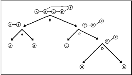
Figure 1 depicts a simple dtree. The root node t of the dtree represents the entire network. To decompose this network, the dtree instructs us to condition on variable B, called the cutset of root node t. Conditioning on a set of variables leads to removing edges outgoing from these variables, which for a cutset is guaranteed to disconnect the network into two subnetworks, one corresponding to the left child of node t and another corresponding to the right child of node t; see Figure 1. This decomposition process continues until a boundary condition is reached, which is a subnetwork that has a single variable.

We will now present some notation needed to define additional concepts with regard to a dtree. The nota­ tion tz and tr will be used for the left child and right child of node t, and the function vars will be extended to internal nodes t: vars ( t ) d:;f vars ( tz ) Uvars ( tr ). Each node in a d tree has three more sets of variables associ­ ated with it. The first two of these sets are used by the RC algorithm, while the third set is used to analyze the complexity of the algorithm.

Definition 2 The cutset of internal node t in a dtree is: cutset ( t ) d:;f vars ( tz ) n vars ( tr ) - acutset ( t ) , where acutset ( t ) is the union of cutsets associated with ances­ tors of node t in the dtree. The context of node t in a dtree is: context ( t ) d:;f vars ( t ) nacutset ( t ) . The cluster of node t in a dtree is: cutset ( t ) U context ( t ) if t is a non-leaf, and as vars ( t) if t is a leaf.

The width of a dtree is the size of its largest cluster -1. It is known that the minimum width over all dtrees for a network is the treewidth of corresponding network [3]. The context width of a dtree is the size of its largest context. Moreover, the minimum context width over all dtrees is the branch width of corresponding network

Algorithm 1 RC ( t ) : Returns the probability of evi­

dence e recorded on the dtree rooted at t. 1: If t is a leaf node, return LOOKUP(t) 2: y .-recorded instantiation of context(t) 3: If cache,[y] of nil, return cachet[y] 4: p .... 0 5: for instantiations c of uninst. vars in cutset(t) do 6: record instantiation c 7: p ._ p + RC(tt)RC(tr) 8: un-record instantiation c 9: cache, [y] ._ p 10: return p

Algorithm 2 LOOKUP ( t )

X <-variable associated with t if X is instantiated then x ._ recorded instantiation of X u � recorded instantiation of .. X''s parents return Pr(xlu) e l s e return 1

[19]. It is also known that the treewidth is no more than a constant factor from branchwidth [19].

The cutset of a dtree node t is used to decompose the network associated with node t into the smaller net­ works associated with the children of t. That is, by conditioning on variables in cutset ( t ) , one is guaran­ teed to disconnect the network associated with node t. The context of dtree node t is used to cache results: Any two computations on the subnetwork associated with node t will yield the same result if these compu­ tations occur under the same instantiation of variables in context ( t). Hence, a cache is associated with each internal dtree node t, which stores the results of such computations ( probabilities ) indexed by instantiations of context ( t ) . This means that the size of a cache as­ sociated with dtree node t can grow as large as the number of instantiations of context ( t). The total space requirement of RC is then Lt ll context ( t ) ll , where II S II represents the number of instantiations of variables S.

2.2 INFERENCE USING RC

Given a Bayesian network and a corresponding dtree with root t, the RC algorithm given in Algorithm 1 can be used to compute the probability of evidence e by first "recording" the instantiation e and then calling RC(t), which returns the probability of e.

Note that Line 9 is where space is used by RC as it is on this line that a cache entry is filled. When ev­ ery computation is cached, RC uses O ( nexp ( w )) time, where n is the number of nodes in the network and w is the width of used dtree. This corresponds to the complexity of JT algorithms, assuming that the dtree is generated from a jointree, and to VE algorithms,

Table 1: Space/Time Requirements for Various Formalisms. The time for Hugin is broken down into the time to compile a jointree (excluding triangulation), and the time to propagate. The experiments used a Pentium 4, 2.4 Ghz processor, with 512 MB RAM.

Network	Hugin ( sec )	Hugin (MB)	SS (MB)	VE (MB)	RC ( sec )	RC Cache (MB)
barley	4.987+1.522	151.137	10.499	140.637	6.43	11.002
diabetes	3.245+0.661	88.147	4.731	83.417	3.044	5.334
mildew	1.732+0.561	74.895	1.91	72.985	2.434	1.907
water	0.961+0.320	30.221	3.778	26.443	1.402	3.871
munin3	2.133+0.320	27.428	3.677	23.752	1.633	5.86
munin4	5.898+1.423	123.353	13.951	109.402	6.76	13.281
link	9.264+3.325	318.502	12.036	306.466	17.936	14.54
pigs	0.391+0.080	6.361	0.95	5.412	0.351	1.02
alarm	0.020+0.000	0.01	0.002	0.008	0.01	0.001
b	0.070+0.070	7.276	1.055	6.221	0.43	1.008

assuming that the dtree is generated from an elimina­ tion order [ 3]. As for space requirements under full caching, RC uses O(nexp(we)) space where We is the context width of used dtree (We :":: w + 1) .1

Suppose now that the available memory is limited and we can only cache a subset of the computations per­ formed by RC. The specific subset that we cache can have a dramatic effect on the algorithm's running time. A key question is then to choose that subset which minimizes the running time, a problem referred to as the secondary optimization problem. This problem has been addressed in [1], which also discusses a version of RC that not only computes the probability of evi­ dence e, but also posterior marginals over families and, hence, posterior marginals over individual variables 2

3 MEMORY USAGE IN RC

We start with our first analysis of RC which focuses on its space requirements under full caching. We were prompted to look into this issue after realizing that some networks which could not be solved by VE or JT methods due to space limitations were solved relatively easily by RC without a need to invoke its time-space tradeoff engine, i.e., these networks were solved under full caching without hitting the same memory limits. This was mostly true for the genetic linkage networks that we discuss in Section 6, whose severe memory requirements have prompted another line of research into time--space tradeoffs [ 7; 8].

We start our analysis by pointing out that one can talk about three measures of space requirements for VE and JT algorithms. In particular, given an elimination

1 Note, however, that RC does not cache results at leaf nodes, so the size of contexts at leaf nodes are not relevant in practice.

2The version of RC in [1] uses a decomposition graph (dgraph ) , which is basically a set of dtrees that share struc­ ture.

order 7l' and a corresponding jointree T, one can define the following space models:

JT /Hugin [11/: Requires one table per cluster and another per separator in the join tree T.

JT/Shenoy-Shafer [20/: Requires one table per separator in the jointree T (assuming that we will only perform the inward pass, otherwise, two ta­ bles per separator).

VE [4/: Requires one table for each cluster con­ structed when eliminating a variable in 7l'. Note that this is no less than the space needed for the cluster tables of Hugin (which is the one we re­ port) and can be a lot more. This is the measure used in [8].

To get a feel of these space requirements on some real­ world networks, we list in Table 1 these requirements for some networks from [2 ; 9]. It should be obvious from this table that the JT /Shenoy-Shafer model is much more space efficient than JTfHugin and VE.3 Note that the space requirements of VE are worse than what is shown in the table since a jointree contains fewer clusters than those created by VE. Note also that JT /Shenoy-Shafer and RC are almost the same as far as space requirements are concerned. We will next provide an analytic explanation for this. Before we do this, we point out that Table 1 shows the time to perform the inward pass on a jointree using Hugin system ( www.hugin. com), a C++ implementation, and the time needed to run RC using the SAMlAM system (http://reasoning. cs. ucla. edu/samiam/), a JAVA im­ plementation. Hugin is about twice as fast on these networks. All comparisons in this table are based on an elimination orderfjointree constructed by Hugin, which is then converted to a dtree by SAM!AM.

30ne can develop a special implementation of VE which requires less memory than standard VE; see [6, Sectiom 10.3].

Table 2: Dead Caches in RC.

Network	Full (MB)	Useful (MB)
barley	35.579	11.002
diabetes	13.364	5.334
mildew	4.139	1.907
water	9.159	3.871
munin3	14.187	5.86
munin4	32.641	13.281
link	21.036	14.54
pigs	1.508	1.02
alarm	0.005	0.001
b	5.704	1.008

One can analytically show that the JT /Shenoy-Shafer model would require less space than the JT /Hugin and VE models, given that each separator is contained in its neighboring cluster, and given that the number of separators is one less the n um b e r of clusters in a join­ tree. But what explains the correspondence between the space requirements of JT /Shenoy-Shafer and RC?

As was shown in [3], the structure of a dtree and its clusters form a jointree. In fact, it is a binary join­ tree since each cluster will have at most 3 neighbors [14]. Moreover, it was shown in [3] that the contexts of a dtree correspond to the separators of induced join­ tree. This shows analytically that RC on a dtree T, and JT /Shenoy-Shafer on the binary jointree induced by T, should require the same space. But binary join­ trees are known to take much more space than non­ binary ones, and the jointrees in Table 1 are in fact non-binary. Hence, the expectation is that RC should require more space than JT /Shenoy-Shafer since the dtree that SAMIAM constructs based on a non-binary jointree is binary and, hence, must require more space. We note, however, that the space requirements for RC in Table 1 are after removing dead caches. Specifically, if a dtree node t has context ( t) which is a superset of the context of its parent node, then the cache asso­ ciated with node t is called dead as its entries will never be looked up [3]. Hence, there is no need to cache at node t, therefore, reducing the space require­ ments of RC. Table 2 provides some data on the sig­ nificant amount of memory reduced due to removing dead caches. Hence, even though dtrees correspond to binary jointrees, they do not suffer from the space disadvantage of binary jointrees due to the removal of dead caches.4

Before we close this section, we point to Table 3 which depicts some networks from genetic linkage analysis to be discussed later. It is these networks that prompted us to look into the space requirements of RC under full

4The notion of dead caches can be applied to jointrees, allowing one to avoid storing some separator tables without affecting the running time. This works, however, only if one is interested in inward-pass propagation: the separators will be needed in case an outward-pass is performed.

Table 3: Space for Genetic Linkage Networks.

Network	Hugin (MB)	SS (MB)	VE (MB)	RC (MB)
EA8	3.609	0.822	2.786	2.37
EA9	229.786	20.777	209.009	26.25
EA10	320.013	48.064	271.949	166.63
EA11	1,144.075	129.135	1,014.94	112.10
EB6	24,485.118	4,136.345	20,348.773	131.71
EB7	17,669.819	3,984.558	13,685.261	420.34
EBB	6,078.274	301.371	5,776.903	41.96
EB9	277.12	22.121	254.999	43.03
EB10	12,571.118	2,183.242	10,387.876	1115.81
EC6	213.252	17.498	195.754	5.67
EC7	81.856	6.639	75.216	9.70

caching as their space under VE/JT is so demanding that it requires some time-space tradeoff to be invoked under these formalisms [7; 8]. Yet, RC was able to handle them all under full caching. We note here that the dtrees used in this table are not built based on the corresponding jointree, but directly from a min­ fill elimination order as described in [3]. Hence, the space requirements of RC and JT /Shenoy-Shafer did not correspond in this table as they did in Table 1.

4 REPRESENTING CPTS IN RC

One of the key properties of RC is that it does not require any particular representation of conditional probability tables ( CPTs). Specifically, as shown by Algorithm 1, the only function that depends on the CPT representation is LOOKUP, which is given in Al­ gorithm 2. LOOKUP is called on a leaf node t corre­ sponding to network variable X only after all its par­ ents U have been instantiated to u. If before the call, X is instantiated to x, LOOKUP returns Pr(x[u), oth­ erwise, it returns 1. Hence, whether the CPT for X is a table, a decision tree, a set of rules, a formula, or a noisy-or model, that does not affect the statement of the algorithm. As for time complexity of RC, that also remains the same as long as the probability Pr(x[u) can be retrieved in constant time.

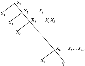
This flexibility of RC with respect to the representa­ tion of CPTs can have a dramatic effect on its space re­ quirements compared to other methods. Consider for example a simple network where variables X1, .. . , Xn are the parents of variable Y. Figure 2 depicts a d tree for this network, with the cutset (left) and context (right) shown next to each dtree node. Since the context of each node is a superset of the context of its parent, all caches in this dtree are dead. Hence, RC does not cache any results in this case, requiring no space whatsoever except that needed to store the CPTs. Hence, if the CPT for node Y has a represen­ tation which is linear in n, then the space complexity of RC on this network is linear in n.

More generally, let N be a Bayesian network with a polytree structure with m nodes, where each node has up to n parents. There is a dtree for N under which RC requires O(m) space for caching, and O(m exp(n)) time. Thus, although the worst-case space complexity of RC is exponential in branchwidth, which is n in this case, this is not necessarily the best-case complexity.

We tried to use Netica and Hugin, both of which are based on jointrees, to construct a network with ternary variables X1, . . . , X 2 0, and binary variable Y which is a noisy-or of its parents X1, . . . , X 2 oOn a Windows 2000 platform with 1 GB of RAM, neither Netica nor Hugin were able to create this network, both running out of memory as we tried to add the 17 t h parent of Y. The reason for this is that these systems will have to convert the noisy-or model to a tabular CPT be­ fore they can use the classical jointree method. It is true that there are new variations on the jointree al­ gorithm which attempt to deal with this problem by adopting non-tabular representations, but these ex­ tensions require serious algorithmic changes as they have to propose algorithms for replacing classical ta­ ble operations, such as multiplication and marginal­ ization. The key property of RC is that no algorith­ mic changes are needed to accommodate non-tabular CPTs, which is a significant advantage that is mostly enabled by the conditioning nature of the algorithm.

5 UNIT RESOLUTION

We now turn to the important subject of handling determinism in Bayesian network inference. It has long been observed that the presence of many ze­ ros and ones in the network CPTs can be a source of great savings. One of the earliest approaches to handle determinism is the method of zer-o compres­ sion proposed for jointrees [12], which reduces the size of a jointree by eliminating table entries that con­ tain zeros. The method, however, requires that we first build a jointree, and then perform inference on it in order to reduce its size. This method can be extremely effective as long as one can construct the full jointree, which may not be possible for some net­ works. Another recent method for handling logical constraints was proposed for variable elimination [5; 13] and is closely related to the approach we will pro­ pose next for recursive conditioning. We will say more about the relationship between the two approaches later.

The approach we take for handling determinism in RC is based on a key technique in the SAT litera­ ture, known as unit resolution. Given a logical knowl­ edge base (KB) in the form of propositional clauses, unit resolution is a linear time method for deriving logical implications of the KB based on setting the values of some variables, allowing one to efficiently de­ tect variable assignments which are inconsistent with a KB. Unit resolution is a very important part of any Boolean satisfiability engine, where a major portion of the engine's run time is spent doing it [15]. Our use of unit resolution in Algorithm 1 is for detecting in­ stantiations c of cutset variables that are guaranteed to have zero probabilities on Line 7, and then skipping these instantiations.

The input to unit resolution is a KB in the form of clauses, where each clause is a disjunction of literals. Each literal is either positive (X = true) or negative (-,(X= true)), assuming that every variable has only one of two values. Since Bayesian networks usually contain multi-valued variables, we extend the notion of a literal to either a positive literal (X = x ) or a negative literal (X =f. x ) .

A clause is satisfied whenever at least one of its literals is satisfied. The basic concept of unit resolution is that when all but one literal/ in a clause have been falsified, then literal l must be satisfied in order to satisfy the clause. A literal is falsified when the current setting of variables contradict the literal. A positive literal X = x is satisfied by setting the value of X to x. A negative literal X =f. x is satisfied by eliminating the value x from the domain of X.

The first step in utilizing unit resolution by RC is to create a KB from a Bayesian network based on the zero/one CPT entries. This can be achieved by mak­ ing each variable in the network a variable in the KB, and then iterating through each CPT entry to create clauses as follows. Consider the following CPT, where variables A and B have values {1, 2} and variable C has values {1, 2, 3}:

A	B	C	Pr(CIA B) ,	Clauses
1	1	1	1	(C- 1 v A# 1 v B# 1)
1	1	2	0
1	1	3	0
1	2	1	0	(C = 2 VA# 1 VB# 2)
1	2	2	1 0
1	2	3	.2
2	1	1	.8
2 2	1 1	2 3
			0	(C# 3 VA# 2 v B# 1)
2	2	1	.7
2	2	2	.3
2	2	3	0	(C# 3 VA# 2 VB=/- 2)

To generate the clauses in the knowledge base, we be­ gin by iterating through the parent instantiations of the CPT for variable C. Whenever one of the states c of C has a probability of 1 we generate a clause which contains the positive literal C = c, and negative literals A f a, B f b where A = a, B = b is the corresponding parent instantiation. The first two clauses in the above table are generated using this method. Whenever no state c contains a probability of 1, each state which has a probability of 0 will generate a clause. This clause contains the negative literal C f c, as well as the neg­ ative literals A f a, B f b where A = a, B = b is the corresponding parent instantiation. The last two clauses in the above table are examples of this.

We also need the following operations on the KB to support unit resolution: assert(X = x ) , assert(X f x), and retract(X) to remove an assertion and any as­ sertions it leads to based on unit resolution. Whenever the knowledge base receives an assertion or retraction, it updates the affected clauses. Anytime all but one literal in a clause is determined to be falsified, it forces the satisfaction of the last literal by calling assert re­ cursively.

The changes needed in RC are then as follows. The operation of "record instantiation c " on Line 6 of Al­ gorithm 1 is changed so that it asserts instantiation c, and the operation of "un-record instantiation c " on Line 8 is changed to retract the instantiation c. More­ over, Line 7 will be skipped in case the assertion on Line 6 leads to a contradiction due to unit resolution as this implies a case c which has a probability of zero.

We note here that the use of unit resolution has been explored in [5]-and a more general form of constraint propagation has also been explored in [13]-in the context of a variable elimination algorithm, where a KB is also constructed based on the 0/1 probabili­ ties in a Bayesian network. A key difference between these previous approaches and ours is that not only do we exploit unit resolution with respect to the original KB, but also with respect to augmentations of the KB which result from adding further assumptions during conditioning. This provides many more opportunities to discover inconsistencies, which may not exist in the original KB.

We study the effectiveness of our proposed technique for handling determinism in the following section.

6 EXPERIMENTAL RESULTS

We will use networks from two different repositories to display the affect of using unit resolution in con­ junction with RC, and to provide further data on the actual memory requirements of RC under full caching.

We start with networks from the field of genetic link­ age analysis [16], where we use a set of benchmark networks from [7]. The problem here is to compute the probability o f some evidence 'vith respect to a given network, known as the likelihood of the pedi­ gree. We will not discuss the details of these net­ works, except to say that (a) they are quite large, containing up to about 9000 variables; (b) require significant memory, upwards of 20 GB for VE and JT/Hugin on some networks; and (3) contain a signif­ icant amount of determinism. These challenges make the benchmarks especially suitable for evaluating RC across the dimensions discussed earlier. In fact, the memory demands of these networks have prompted an­ other line of research on time-space tradeoffs, which combines variable elimination and conditioning [7; 8]. Yet, as we shall see next, the memory demands of RC under full caching are modest enough to allow the handling of these networks without invoking its time-space tradeoff engine.

Table 4 depicts the results of running RC on the ge­ netic linkage networks from [7], in addition to report­ ing the performance of SUPERLINK 1.0 [7] and SU­ PERLINK 1.1 [8] on these networks. We note here that SUPERLINK is currently the most efficient soft­ ware system for genetic linkage analysis, and is dedi­ cated to this problem, although it is based on proba­ bilistic inference using a combination of variable elim­ ination and conditioning. Hence, gauging our results with respect to SUPERLINK is quite revealing.

A number of observations are in order about the re­ sults in Table 4. First, the results reported for RC and SUPERLINK 1.1 are on a Linux system, with a 2.4 GHz Xeon processor, and 1.5 GB of RAM, while the results for SUPERLINK 1.0 are for a slower ma­ chine with 2 GB of RAM and are adapted from [ 7] (we could not obtain a version that runs on the above plat­ form). Second, given this memory constraint, many of the networks in Table 4 are beyond the limits of stan­ dard methods based on VE and JT /Hugin and, some­ times, JT /Shenoy-Shafer; see Table 3. Third, the RC results are based on SAMIAM, using a special imple-

Table 4: Genetic Linkage Analysis: Experimental Results.

File		Number Variables	RC Time (sec)	Superlink 1.0 I	Time (sec} 1.1	Dtree Cache Size (MB)	KB Size (clauses:literals)	Actual RC Calls	Ratio RC Calls
EA5	noKB KB	2092	0.2 0.2	1.2	0.2	0.10	1588' 4500	ll6.233 70,175	1.66
EA6	noKB KB	2491	0.5 0.4	4.7	1.6	0.28	1838' 5ll2	293,507 ll3,699	2.58
EA7	noKB KB	2928	1.0 0.4	3.0	0.6	0.66	2ll4 ' 5812	651,151 94,583	6.88
EA8	noKB KB	3790	3.1 1.3	21.0	3.3	2.37	2410' 6424	1,944,307 245,429	7.92
EA9	noKB KB	7747	175.4 23.8	8510.2	356.4	26.25	4600' 11784	64,926,609 3,347,807	19.39
EA10	noKB KB	7970	685.9 201.1	10446.3	451.7	166.63	4762' 12200	325,061,629 17,258,401	18.83
EA11	noKB KB	9027	710.4 195.0	> 100 hours	12,332.0	112.10	5286' 13424	245,669,493 14,358,315	17.11
EBO	noKB KB	1926	0.2 0.2	2.6	0.1	0.11	1751' 5121	100,773 33,153	3.04
EB1	noKB KB	2317	0.3 0.2	2.6	0.2	0.18	2025 ' 5723	157,915 47,499	3.32
EB2	noKB KB	3919	0.6 0.2	82.6	0.7	0.39	2961' 7831	396,027 83,307	4.75
EB3	noKB KB	4710	48.3 11.6	437.6	4.1	10.00	3537 ' 9233	28,593,739 2,102,409	13.60
EB4	noKB KB	5088	19.1 13.0	17.3	5.5	5.80	3763' 9785	7,164,295 1,188,043	6.03
EB5	noKB KB	5483	71.7 8.0	278.8	12.4	23.82	4007' 10297	29,839,491 1,574,619	18.95
EB6	noKB KB	5860	981.1 281.9	935.9	15.5	131.72	4220' 10787	477,764,683 43,572,385	10.96
EB7	noKB KB	6240	3107.8 610.3	902.8	4.0	420.34	4564' 11595	1,379,395,611 83,540,347	16.51
EB8	noKB KB	6623	1009.1 54.4	288.2	18.0	41.96	4945' 12577	322,142,481 4,474,309	72.00
EB9	noKB KB	7039	1656.2 123.7	114.0	27.9	43.03	5126 ' 13011	713,453,263 18,814,149	37.92
EB10	noKB KB	7428	> 3600.0 650.4	2901.3	85.1	1115.81	5473' 13994	1,452,529,921 76,309,713	19.03
EC5	noKB KB	1194	26.7 5.6	44.1	1.6	5.89 5.89	788' 2192	8,612,171 577,315	14.92
EC6	noKB KB	1200	29.8 6.3	35.3	124.9	5.67 5.67	704' 1968	11,896,861 1,298,445	9.16
EC7	noKB KB	1321	59.7 25.0	102.6	123.0	9.70 9.70	762' 2108	19,053,079 4,742,827	4.02

mentation which works in log-space given the small numbers involved in genetic linkage analysis. Finally, all dtrees used in these experiments were created from elimination orders based on the min-fill heuristic [3].

Note that each row in Table 4 contains two lines, one for standard RC (noKB) and another for RC with unit resolution (KB). The running time, actual num­ ber of recursive calls, and the ratio of recursive calls, noKB/KB, is also reported. The running time for RC is for two likelihood calculations, while the other val­ ues are for a single calculation. Some computations could be stored from one calculation to the next [7], however our current implementation does not use this speedup. Based on this table, it is obvious that the use of unit resolution has only improved performance, considerably in many cases, with some minor excep­ tions where standard RC was so fast that the use of unit resolution was not justified. To highlight some im­ provements, consider EB10 which could not be solved within 1 hour, but was then solved in under 10 min- utes using unit resolution. For EB9, the running time dropped from 1656 to 124 seconds. The last column in Table 4 reports on the factor of reduction in the num­ ber of recursive calls made by RC, showing a factor of 72 for EB8.

Another key point to observe is the size of KBs gener­ ated for these networks, which contained up to about 5000 clauses. This is a relatively large number of clauses, at least by SAT standards, yet is not as large as some of the other networks we shall consider later.

The final set of remarks relating to Table 4 are with regards to gauging the running time of RC against SU­ PERLINK, the most efficient software system for ge­ netic linkage analysis. We note here that RC running times only include two likelihood calculations, while SUPERLINK running times additionally include the time to preprocess and create an ordering, as this is the number reported by SUPERLINK. The prepro­ cessing phase used by RC reads in the genetic files, converts it to a Bayesian network, and then simplifies

Table 5: KB Compared with No KB.

Network	RC KBj		RC \No KB)		K/3 Size		RC Cache	Ratio
	Seconds	RC Calls	Seconds	RC Calls	Clauses	Literals	(MB)	RC Calls
rnuninl	65.875	404,101	351.896	1,059,450,113	8334	26500	452.9	2621.75
munin3	2.544	201,559	3.865	24,743,617	31826	94198	8.4	122.76
munin4	9.293	986,675	16.844	101,264,503	39485	122441	33.5	102.63
water	1.292	31,097	1.422	8,751,957	6362	35249	2.5	281.44
munin2	14.270	582,961	2.383	14,596,471	31365	93775	4.6	25.04
pigs	2.844	1,049,061	0.431	1,717,165	2368	7104	1.4	1.64

it as discussed in [7].5 This phase is currently using unoptimized Java code, and along with the dtree gen­ eration, took 6 seconds on EA7, 20 seconds on EB6, and 51 seconds on EAll. It should be noted that this only needs to be done once for any number of likelihood calculations, which geneticists would be in­ terested in running. Even after taking this into con­ sideration, RC's numbers appear competitive with the newer version of SUPERLINK on this dataset (see, for example, EA9-11, EB5, EC6-7).

We note here that SUPERLINK 1.1 is quite recent (the paper to appear). It is based on a new variable ordering technique, which depends on randomization, and appears to be extremely effective [8]. This im­ provement is orthogonal to the improvement shown by using unit resolution, in that by finding better or­ derings, we could abo generate better dtrees, therefore lifting the additional benefits of SUPERLINK 1.1 to RC. We are currently investigating this direction. We finally note that the benchmarks in [7] included addi­ tional networks that we omitted here, as they were too easy, requiring less than a second each.

We now consider another set of networks from a dif­ ferent suite [2], where we will only run one probability calculation. These networks contain even more deter­ minism than the genetic linkage networks, to the point where unit resolution stops being helpful in some cases due to the significant size of KBs. Specifically, consider Table 5 and the munin2 network, which generates a KB with 31,365 clauses. RC with unit resolution re­ duced the number of recursive calls by a factor of"" 25, yet it slowed down the overall running time by a factor of"" 6. A slowdown is also observed for pigs since the initial running time was very small to start with. An impressive case is the one concerning muninl, where unit resolution reduced the number of recursive calls by a factor of "'=' 2, 600, and reduced the running time from "'=' 352 to 66 seconds. One key observation about these networks is the significant size of KBs, which explains why the reduction in running time is not pro­ portional to the reduction in number of recursive calls.

5This involves value and allele exclusion, variable trim­ ming, and merging variables.

We note here that our implementation of unit resolu­ tion is quite straightforward, especially that it contains multi-valued variables. There is very little published literature on optimization techniques for unit resolu­ tion with multi-valued variables (as opposed to binary variables) and we have yet to invest in such techniques. The promising experimental results we report in this section, however, appear to justify such an investment.

7 CONCLUSIONS

This paper rests on two key contributions. First, an analytic and experimental study of the space require­ ments of RC under full caching, suggesting that it is one of the most space--efficient algorithms for exact in­ ference in Bayesian networks, aside from its ability to allow a smooth tradeoff between time and space. Sec­ ond, a principled approach for handling determinism in probabilistic inference, which builds upon progress made in the SAT community. Both contributions are supported by experimental results on a variety of real­ world networks, including some very challenging net­ works from the field of genetic linkage analysis. The combination of unit resolution with RC in particular shows a lot of promise in terms of time complexity, suggesting some new directions of research on the in­ terplay between probabilistic and symbolic reasoning.

Acknowledgements

This work has been partially supported by NSF grant IIS-9988543 and MURI grant N00014-00-1-0617.

References

1. David Allen and Adnan Darwiche. Optimal time--space tradeoff in probabilistic inference. In IJCAI-2003, 2003.
2. Bayesian Network Repository. http:/ fwww.cs. huji.ac.il/labs/compbio/Repository /, URL.
3. Adnan Darwiche. Recursive conditioning. Artifi­ cial Intelligence, 126(1-2):5--41, 2001.

1. Rina Dechter. Bucket elimination: A unifying framework for probabilistic inference. In Proceed­ ings of UAI-96, 211-219, 1996.
2. Rina Dechter and David Larkin. Hybrid Process­ ing of Beliefs and Constraints. In Proceedings of UAI-01, 112-119, 2001.
3. Rina Dechter. Constraint Processing. Morgan Kaufmann Publishers, Inc., 2003.
4. Ma'ayan Fishelson and Dan Geiger. Exact ge­ netic linkage computations for general pedigrees. Bioinformatics, 18(1):189-198, 2002.
5. Ma'ayan Fishelson and Dan Geiger. Optimiz­ ing exact genetic linkage computations. In RE­ COMB'03, 2003.
6. GeNie. http:/ / www 2.sis.pitt.edu;-genie/, URL.
7. Cecil Huang and Adnan Darwiche. Inference in belief networks: A procedural guide. In­ ternational Journal of Approximate Reasoning, 15(3):225-263, 1996.
8. F. V. Jensen, S.L. Lauritzen, and K.G. Olesen. Bayesian updating in recursive graphical models by local computation. Computational Statistics Quarterly, 4:269-282, 1990.
9. Frank Jensen and Stig K. Andersen. Approxima­ tions in Bayesian belief universes for knowledge based systems. In Proceedings of UAI-90, 162169, 1990.
10. David Larkin and Rina Dechter. Bayesian infer­ ence in the presence of determinism. In Proceed­ ings of the Ninth International Workshop on Ar­ tificial Intelligence and Statistics, 2003.
11. Vasilica Lepar and Prakash P. Shenoy. A compari­ son of lauritzen-spiegelhalter, hugin, and shenoy­ shafer architectures for computing marginals of probability distributions. In Proceedings of UAI98, 32B-337, 1998.
12. Matthew W. Moskewicz, Conor F. Madigan, Ying Zhao, Lintao Zhang, and Sharad Malik. Chaff: Engineering an efficient sat solver. In 39th Design Automation Conference, 2001.
13. Jurg Ott. Analysis of Human Genetic Linkage. The Johns Hopkins University Press, 1999.
14. Judea Pearl. Probabilistic Reasoning in Intelligent Systems: Networks of Plausible Inference. Mor­ gan Kaufmann Publishers, Inc., 1988.
15. N. Robertson and P. D. Seymour. Graph minors IV. tree-width and well-quasiordering. J. Combin. Theory Ser. B, 48:227-254, 1990.
16. N. Robertson and P. D. Seymour. Graph minors X: Obstructions to tree-decomposition. J. Com­ bin. Theory, Ser. B, 52:153-190, 1991.
17. Prakash P. Shenoy and Glenn Shafer. Propa­ gating belief functions with local computations. IEEE Expert, 1(3):43-52, 1986.
18. Nevin Lianwen Zhang and David Poole. A simple approach to bayesian network computations. In Proceedings of UAI-94, 171-178, 1994.