Nonuniform dynamic discretization in hybrid networks

Alexander V. Kozlov

Department of Computer Science Stanford University

Stanford, CA 94305-9010 e-mail: [email protected]

Abstract

We consider probabilistic inference in general hy­ brid networks, which include continuous and dis­ crete variables in an arbitrary topology. We re­ examine the question of variable discretization in a hybrid network aiming at minimizing the in­ formation loss induced by the discretization. We show that a nonuniform partition across all vari­ ables as opposed to uniform partition of each vari­ able separately reduces the size of the data struc­ tures needed to represent a continuous function. We also provide a simple but efficient procedure for nonuniform partition. To represent a nonuni­ form discretization in the co m pu te r memory, we introduce a new data structure, which we call a Bi­ nary Split Partition (BSP) tree. We show that BSP trees can be an exponential factor smaller than the data structures in the standard uniform discretiza­ tion in multiple dimensions and show how the BSP trees can be used in the standard join tree algo­ rithm. We show that the accuracy of the inference process can be significantly improved by adjusting discretization with evidence. We construct an it­ erative anytime algorithm that gradually improves the quality of the discretization and the accuracy of the answer on a query. We p ro v i d e e m p i r i c a l evidence that the algorithm converges.

1 INTRODUCTION

A Bayesian network is an efficient representation of a joint p r o b a bi l ity distribution over domain variables. Bayesian networks allow intuitive causal interpretation of dependen­ cies as well as efficient algorithms for probabilistic infer­ ence. In particular, we can obtain answers for queries about the probabilities of some events given information about others. Bayesian networks are becoming a popular tool for reasoning under uncertainty and have been used in a num­ ber of practical systems.

Daphne Koller

Department of Computer Science Stanford University Stanford, CA 94305-9010

e -m ai l

: [email protected]

Although there exists a number of efficient inference al­ gorithms and implementations for probabilistic reason­ ing in Bayesian networks with discrete variables (for example, [Pearl, 1988, Lauritzen and Spiegelhalter, 1988, Li and D'Ambrosio, 1994, Dechter, 1996]), few algo­ rithms support efficient inference in hybrid Bayesian net­ works, Bayesian networks where continuous and discrete variables are intermixed. Exact probabilistic inference in hybrid networks can be reduced to taking multidi­ m e n sio n al integrals in the same way that exact i n f er ­ ence in discrete networks can be reduced to computing s u m s [Li and D'Ambrosio, 1994, Dechter, 1996]. How­ ever, computing integrals exactly is possible only for a re­ stricted class of continuous functions.

For example, one of the hybrid Bayesian network classes where exact probabilistic inference is possible are networks with Conditional Gaussian (CG) density functions [Lauritzen and Wermuth, 1989, Lauritzen, 1992, Olesen, 1993]. Probabilistic inference in these networks is polynomial in the number of continuous variables. How­ ever, the CG limitations on the dependencies between vari­ ables obstruct the application of hybrid networks in many domains. In many practical problems we have dependen­ cies substantially different from those encompassed by the CG model. For example, we c an n o t model a discrete sen­ sor of a continuous variable, say a fire alarm activated by smoke concentration, since continuous variables are not al­ lowed to have discrete descendants in CG hybrid networks.

Given that we want to reason with a more general class of networks and distributions than CG, we need to design approximate methods for inference in hybrid networks. A useful extension of the previous technique is to decompose an arbitrary conditional probability distribution into sev­ eral CG distributions, and to represent continuous functions as the sums of CG functions [Driver and Morrel, 1995, Alag and Agogino, 1996]. The price one pays is a fast growth of the number of terms in the sums during prob­ abilistic inference. In a join tree, for example, each time a clique potential is multiplied by a message, the number of terms in the resulting sum is the product of the number of

terms in each of the factors before the multiplication, thus making the number of terms in the s u m s grow exponen­ tially with the path length. In addition to this p ro b l e m , the initial a ppro x im a ti on of an arbitrary continuous function by a sum of CGs can also present a computational chal­ l en g e. The number of terms in such a decomposition can be p r o h ibiti v e l y large, and probabilistic inference compu­ tationally int r acta bl e.

The other approach, the one most c o m m o n ly used in prac­ tice, is to discretize all variables in a network. Tradition­ ally, we would discretize each variable separately and rep­ resent the conditional probabi li t i es of the nodes in a net­ work and the clique potentials as multidimensional tables. In this a p p r o ach , the size of a clique potential table is the product of the number of d i s cr et ize d values f or the vari­ ables participating in the clique. Since the nu m be r of vari­ ables in a clique can be quite large, we usually cannot af­ ford to discretize the variables as finely as we would like. As a consequence, we incur significant error relative to the exact solution.

In this paper, we propose an alternative approach. Rather than discretizing each variable separately, we discretize a continuous function on its entire multidimensional domain at once. Thus, we can adjust our discretization to the sh a pe of the function, providing a fi ne r partition in places where the function changes rapidly, w h i l e l e a vi ng relatively "flat" regions at a very r o u gh level of granularity. We show t h a t the nonuniform discretization allows us to provide much g re a t e r accuracy using the same number of partitions of the function domain.

To represent one of such nonuniform discretization, we introduce a new data structure, a Binary Split Partition (BSP) tree. A BSP tree r e p r esents a recursive binary par­ tition of a function domain and is similar to the quadtrees or octrees used in gr a phi cs for representing space objects [Samet and We b be r , 1988]. 1 In a BSP t r ee, we restrict the partitions of the multidimensional domains to binary splits by a plane orthogonal to one of the coordinate axes. We show that, for a given number of partitions, BSP trees come very close to the optimal nonuniform discretization of a multidimensional probability function. In particular, t h e y are s i g n i fi c an t ly more compact than the traditional repre­ sentation of continuous functions by multidimensional ta­ bles.

Of course, we don't want to discretize the entire joint den­ sity function at once. We therefore propose a n a p p roa c h where the density function in each clique in a join tree is discretized using our nonuniform discretization. We show how the traditional join tree algorithm ca n b e a d apted to do i n f e r e n c e with the BSP t r e es , and how the probabilistic

1 Recursive partition of multivariate domains have been also used in multivariate regression and machine learning [Breiman et al., 1984, Moore, 1991].

inference steps can be a p propr i a t ely interleaved with dis­ cretization steps.

Like most other approximation techniques, our approach targets the discretization to do well on the most likely sce­ narios. As a consequence, it i s likely to incur large er­ rors in the case of unlikely evidence. We co u l d refine our discretization so that it remains accurate under all circum­ stances, but the resulting discretization is likely to be in­ feasibly large. R a th e r , we propose an a p p ro ach that adjusts the discretization to reflect the observed evidence and the needs of the query. An o p tim al implementation of this pro­ cess requires that we base our discretization on the pos­ terior pr o b ab i l i t y distributions. Since we do not have ac­ cess to this posterior, we execute an iterative p ro c e d u re , in which the accuracy of ou r pr edict i o n s and the quality of our discretization increases with each iteration. We show em­ pirically that the results of this p r o c edu r e converge quickly to the exact results.

2 NONUNIFORM DISCRETIZATION

A discretization is conventionally understood as a subdivi­ sion of the range of a continuous variable into a set of sub­ ranges. If each of t h e variables is discretized separately, the computational complexity of probabilistic inference grows as the number of discretization subranges, or the number of states pe r variable, to the power of the induced width of the graph [Dechter, 1996]. Since the induced width can be as large as 20 for pr actic a l networks, we want to keep the number of discretization subregions low while preserving m o s t of the information in the discretized function.

We w ou l d like to discretize only the regions of a function that contribute to the structure of the joint probability distri­ bution. By providing more detail about the more relevant parts of t h e space, we can provide a much more accurate picture of the distribution than if we discretize each vari­ able separately. In this section, we generalize the notion of a discretization. We begin by considering the problem of d i sc re ti z ing a si n g l e function on a mult i d i mens i o n al do­ main. In later sections, we will a p p l y these ideas to de­ c o m p o sed pro ba bility distributions, such as those found in a Bayesian network.

All treatment in this part is based on the r ela ­ tive entropy or Kullback-Leibler (KL) d i st a n c e be­ tween two p r oba b i l ity densi t y functions J( x) and g( x) [Cover and Thomas, 1991 ]:

as a metric for the error introduced by the discretiza­ tion. There are many justifications for the use of relative e n tr o p y as a distance metric between distribu­ tions [Cover and Thomas, 1991], including several of u s e ­ ful p r op e rt ies that we will use throughout the paper.

Our first task is to find the optimal discretization and op­ timal values for the discretized function. Without loss of generality, we consider discretizing a continuous function defined on a hypercube n = [0, l)n . To compare the results for different discretizations, we need a formal definition.

Definition 2.1: A discretization 'D of a hypercube n = [0, l]n i s a p iece w i se constant function iD(x1, ... ,xn) from n to a finite set of integers from 1 to m. The function defines mutually exclusive and collectively exhaustive set of subregions { w;, i = 1, .. . , m} in f.!. I

If a probability density function fD(x1, ... ,xn) is con­ stant in each of the subregions w;, we call it a dis­ cretized function on the discretization 'D. The follow­ ing theorem proves that the optimal value for the dis­ cretized function fD ( x 1, . . . , Xn ) is the mean of the func­ tionf(x1, ... ,xn) in each of the subregionsw;.

Theorem 2.1: Given a discretization 'D o f a region n. the minimum KL distance between a probability den­ sity function f(x1, ... , xn) and a discretized function fD(Xt, ... , xn) is achieved by the discretized function / D(Xt, ... , xn) which is piecewise constant and in each of the subregions w; is equal to the mean of the function f(xt, ... ,xn) in the corresponding subregion w;. The KL distance to any other piecewise constant on 'D f un c ­ tion fD(Xt, ... , xn) which is also piecewise constant and in each of the subregions w; is g i ve n by the sum of KL dis­ tancesfromfD(x1, ... ,xn)to / D(xl, ... ,xn)andfrom / v(xt, ... , xn)tof(xt, . .. ,xn)·

This ts a consequence of well-known decom­ position properties of relative entropy dis­ tance [Cover and Thomas, 1 991]. Due to the space restrictions we do not show the proof of the theorem.

Now that we have a procedure to assign values to a dis­ cretized function given the discretization, we need to find a discretization that minimizes the relative entropy error. Be­ low, we provide a simple divide and conquer technique for finding a discretization which is very close to optimal.

To find an optimal discretization of a hypercube n into m subregions we should search through all possible partitions of n into m subregions for a partition that gives us the minimal KL distance between the origi­ nal function f(x1, · · · , Xn) and its discretized function fv ( x 1, ... , Xn ) with optimally assigned values in the sub­ regions. This procedure is computationally intensive even in one dimension and becomes computationally intractable in multiple dimensions. Instead, we propose a simple re­ cursive technique and show that it generates results very close to optimal.

We borrow the idea of a recursive space decomposition from graphics [Samet and Webber, 1988], where quadtree and octree decomposition of twoand three-dimensional spatial respectively are often used for a compressed repre­ sentation of space objects. Both of these data structures have proved to be very efficient computationally.

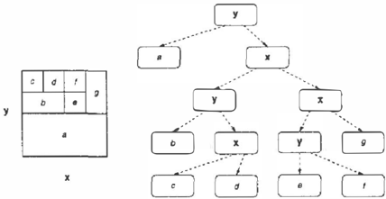
A Binary Split Partition (BSP) tree is a recursive data struc­ ture that represents a hierarchical binary decomposition of a multidimensional function. Each node in the tree repre­ sents a subregion of the function domain and can have two children. Each of the children represents half of the par­ ent's space. The splitting continues from the root of the tree, representing the whole function domain, to the leaves, that carry information about the function in a particular subregion.

We restrict the splits to subdivisions of the space into two halves defined by a plane orthogonal to one of the axes. For e x am p l e , one of the possible BSP trees for a function of two variables x and y is shown in Fig. 1. On the first level, we split the function domain by a line orthogonal to y. On the second level, we leave the left node as a leaf representing the lower half of the xy plane. We split the right one, representing the upper half of the xy plane, by a line orthogonal to x. Each of the children on the third level is split even further.

As a result, the function represented by the BSP tree in Fig. I is constant in the lower half of the xy plane. The discretization has higher granularity in the upper half of the xy plane, where we continue splitting. The BSP tree in Fig. 1 might be useful for representing a function with some structure in the upper half of the xy plane.

To discretize a function, we need heuristic that tells us how to build up a BSP tree: which leaf to split next and in which direction. Since computing the exact contribution to the relative entropy error is computationally expensive for a general function, we use a bound on the KL distance between the function f and its discretization fv based on the function mean / ,the function maximum !max, and the function minimum !min in the given subregion w;:

where l w; I denotes the volume of a discretization subre­ gion w;. The parameters f. !max. !min are estimated by randomly sampling f at several points.

During the discretization process, all l e a v e s are kept in a priority queue. The estimates of the relative entropy error are used to take the leaves out of the queue. A leaf with the largest error estimate is then split first, and the two re­ sulting leaves are put back into the queue. To control the accuracy of our discretization, we also maintain the sum of all estimates for all the leaves in the queue. We stop the discretization process when either the estimate of the error

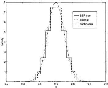
Figure 2: BSP tree (solid line) and optimal (dashed line) dis­ cretization of a normal distribution N(x; 0.5, 0.0025) (dotted line)_ The number of discretization intervals is 16 in both cases. The optimal discretization was found by the gradient descent method.

,., .----�---.

becomes smaller than some fixed parameter {J or the num­ ber of leaves exceeds some fixed number N.

Finding the direction of the optimal split presents a chal­ lenging problem. In an ideal s i t uati on , we would estimate the decrease in the relative entropy distance due to all pos­ sible splits and choose the optimal one. However, to do this exactly, we would need to estimate multidimensional inte­ grals. Instead, we sample several points around the cen­ ter of the subregions w; and pick the direction in which the function changes most, i.e., the coordinate axis along which the ratio !max/ /min is the largest around the center of the subregion w;.

The result of the one-dimensional discretization of a nor­ maldistributionN(x;t-t,a-2) = �.,1 exp(-(x-t-t)2/2u2) V�1UJ with J.l = 0.5 and u = 0.05 is shown in Fig. 2. The algo-

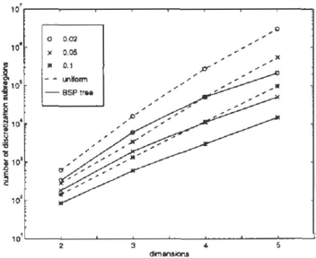
Figure 4: Number of discretization subregions as a function of the n u mbe r of dimensions for BSP tree (solid line) and uniform (dashed line) discretization. The discretization was performed to approximate a multivariate normal distribution proportional to N(L,�-! x;/(n -1) -xn; 0, 0.0025) with relative entropy error 0.02, 0.05, and 0.1. For a large number of dimensions, the BSP discretization performs much better (notice the loga­ rithmic scale for the number of discretization subregions).

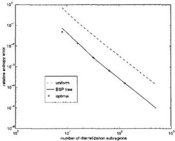
rithm correctly chooses to discretize the regions that have higher derivative and/or are high in probability density. In fact, the discretization obtained with BSP tree is very close to the optimal discretization obtained by the gradient de­ scent method. This is confirmed by Fig. 3, which shows the relative entropy error as a function of the number of dis­ cretization subregions. The error of the BSP tree discretiza­ tion and the optimal discretization is virtually the same for the number of discretization intervals larger than 16. On the other hand, an eq u idis t a n t discretization requires about a factor of 5 more discretization intervals to reach the same accuracy.

BSP trees are even more promising for representing mul­ tidimensional density functions. If a function has sharp ridges, the savings are exponential in the number of

dimensions-we save a constant factor along each of the dimensions. The results of discretizing a multivari­ ate normal distribution proportional to N(L�-l x;/(n1) -Xn; 0, 0.0025) with different relative entropy error are shown in Fig. 4. Given the accuracy, the number of discretization subregions grows much slower for a BSP discretization than for a standard uniform equidistant dis­ cretization of each of the variables separately. We save about a factor of 10 in 5 dimensions.

3 OPERATIONS ON BSP TREES

In this section, we briefly consider summation, multiplica­ tion, and integration of functions represented by BSP trees. We will show in the next section how the BSP trees can be used in the standard join tree algorithm for probabilistic inference.

We assume that the BSP trees are encoded as a tree struc­ ture that uses pointers. Other implementations, that might be more computationally efficient, are possible, but are out of the scope of this paper. We refer the reader to [Samet and Webber, 1 988] for a comprehensive review on this subject

Let us start with the summation of two BSP trees. We will use summation later in our integration algorithm. If the structure of the trees is aligned, i.e., they have exactly the same splits on the same levels, the summation is reduced to a tree traversal. The values at the leaves are summed during the traversal. Tree traversal takes linear time and the computational complexity for the aligned trees is O(N), where N is the number of leaves in a tree.

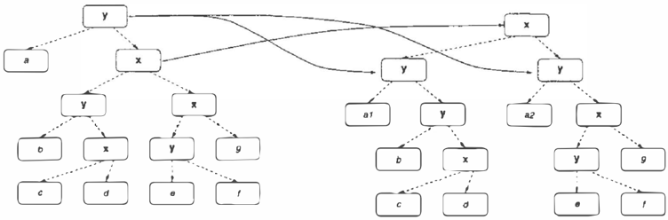
If the trees are not aligned, we need to adjust the structure of one of them by inserting additional nodes. For example, if we want to sum the tree in Fig. I with another tree that has a root split on variable x, we adjust the structure of the first tree as shown in Fig. 5 by moving the x split in the right branch up and by making two additional leaves in the corresponding branches. Complete alignment of the trees takes O(N1 x N2) operations in the worst case, where N1 and N2 are the number of leaves in the first and the second trees respectively.

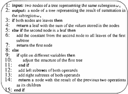
The algorithm for summing two nodes of a BSP tree is shown in Fig. 6. Summation takes O(N1 + N2) opera­ tions in the best and O(N1 x N2) operations in the worst case. Intuitively, if all the splits in both operands are on the same variable, the computational complexity is linear. If the trees are completely misaligned, for example if all the splits in the first tree are on variable x and in the second tree are on variable y, then the computational complexity is quadratic.

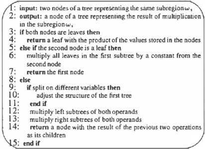
The algorithm for multiplying two nodes of a BSP tree is

shown in Fig. 7. As in the summation algorithm, we have to align the trees when they have different structure. Anal­ ogously, multiplication takes O(N1 + N2) operations in the best and O(N 1 x N2) operations in the w orst case w!len the trees are completely misaligned.

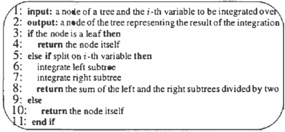
Finally, we consider the integration of a function repre­ sented as a BSP tree over some variable. This is the op­ eration that, in the discrete case, corresponds to variable elimination by summation. Since a leaf represents a con­ stant value of a function over a region, integration of a leaf is reduced to multiplication of the value stored in the leaf by the corresponding multidimensional volume. It is p ossi b le to compute this volume during the process of tree traver­ sal, since the volume of a subregion represented by a child is al w ays half the size of the subregion represented by its parent. The integration algorithm is presented in Fig. 8. In­ tegration also takes O(N1 + N2) operations in the best and O(N1 x N2) operations in the worst case.

Many other algorithms, for such tasks as computing the ex­ pected value of a function, the cross entropy, or the differ­ ential entropy, can be expressed as a simple traversal of the tree, thus taking linear time w ith respect to the size of the tree.

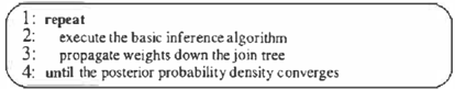
4 BASIC PROBABILISTIC INFERENCE ALGORITHM

We now show how we can integrate our nonuniform dis­ cretization using BSP trees into standard Bayesian net­ work inference algorithms. Our approach will be based on the optimal factoring approach to probabilistic inference [Li and D'Ambrosio, 1994].

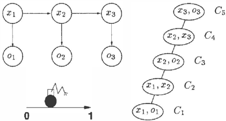
We illustrate our algorithm using an example. Let us as­ sume that we can observe a one-dimensional robot on the interval 0 ::; x ::; 1. Although we do not kno w the robot's position exactly, we kno w the readings of a number of sen­ sors and know that the robot can walk randomly between the observations. The Bayesian network corresponding to this situation is shown in Fig. 9.

If the robot's position x, the first and the second sensor reading is o with probability p(olx) = N(o- x; 0, 0.01). Thus, the first t wo observations are noisy observations of the robot coordinate. The third observation is a discrete noisy observation of the robot in the left halfspace x < 0.5. If the robot position is x, the sensor is likely to give a reading of true with probability ( 1 + exp( 40(x0.5))r 1 .

0

1

Figure 9: A simple hybrid Bayesian network used as an example and its join tree.

The dependence of the robot coordinate at the next obser­ vation on the robot position at the current observation is given by the conditional probabilities p(x3lx2) = N(x3xz; 0, 0.01) and p(x2lx1) = N( x2- x1; 0, 0.01 ). Our prior beliefs about the robot position are uniform: p(xl) = 1. We would like to know the probability distribution of the robot coordinate after three observations.

The join tree corresponding to this net work is show n in Fig. 9. Probabilistic inference with continuous variables can be analyzed in the same optimal factoring approach used in[Li and D'Ambrosio, 1994]. The posterior proba­ bility of the robot coordinate after observations o1, o2, and o3 is:

Computing integrals in the above decomposition corre­ sponds to computing messages in the standard join tree al­ gorithm. Partial sums or integrated conditional probabili­ ties represent messages passed from one clique to another.

This net w ork was chosen so as to allow us to compare the performance of our algorithm to the true ans wers. There­ fore, the net work is exactly solvable up to a normalizing factor given the observations o1, o2, o3 = true:

where the answer was obtained by integrating the joint probability over x1 and x2.

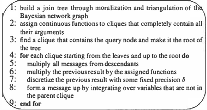
The reformulated join tree algorithm is shown in Fig. 10. For our network, we would first multiply the continuous conditional probabilities p( o 1 l x 1 ) and p( xt) in clique C1, discretize it using our BSP tree construction algorithm, and pass a discretized message to clique C2. The clique C2 will multiply the message by p(x21xt), discretize it, then inte­ grate over x1, and pass it to the next clique C3. The basic operations used in the inference process reduce to the oper­ ations described in Section 3. The process continues until the last clique, C5, receives the discretized message, multi­ plies it by the continuous function p( o 3 l x 3 ) , and discretizes it. Note that the function at a clique is only discretized af­ ter it received the messages from its subtrees, allowing its choice of discretization to be much more informed.

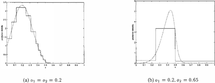
In many cases, this process does very well. For example, as we see in Fig. 11, if our first two observations are the same-o1 = o2 = 0.2-the results of the inference are very close to the exact solution, computed analytically in (3). However, as our observations become more and more unlikely, the accuracy of the results of this basic inference algorithm begins to deteriorate. If, for example, the sec­ ond observation is changed to o2 = 0.65, the results of the inference contain only a single bump (see Fig. 11) and are very different from the exact answer. In the next section we describe how to improve the performance of this algorithm in the case of unlikely evidence.

5 DYNAMIC DISCRETIZATION

To understand why the results of probabilistic inference de­ pend on the probability of evidence p( e), let us consider the decomposition of the KL distance between the true joint probability distribution given by the product of all con­ tinuous functions p(x, e) = Tii p(x;IPa(xi)) and the dis­ cretized joint probability distribution fv( x, e ):

where D(p(xle)llf:v(xle)) is the conditional relative en­ tropy or conditional Kullback-Leibler distance:

The second integral essentially represents a KL distance between the desired answer to a query p( xI e ) and the an­ swer obtained with our discretized network fv(xle). How­ ever, this relative entropy integral is multiplied by p( e). Thus, even if we bound the relative entropy error of the discretization for the whole network byE, the bound on the error of our answer is t / p( e).

Rather than minimizing the KL distance of the full joint probability, as we do by discretizing partial sums, we need to minimize the KL distance:

of the query node q conditioned on the evidence e . Given the evidence, we might want to change the discretization and rediscretize the regions that become probable given the evidence. Thus, we propose a more general metric that will reflect our preferences to discretize some regions more finely than the others.

Definition 5.1: The weighted relative entropy or Weighted Kullback-Leibler (WKL) distance W (f(x)llg(x); w (x)) between the density functions f( x) and g( x) with a strictly positive weight w( x) is defined by:

where we assume that the integral exists. I

The WKL distance reduces to the KL distance if the weight function is constant. Although in general the WKL distance is not even sign definite, the following inequalities hold if the weight w( x) and the function f( x) are discretized using the same discretization V:

The proof follows from considering the contributions from each of the subregions Wj. These inequalities follow from bounding each contribution by maximum/minimum weight times the corresponding contribution to the relative en­ tropy.

5.1 WEIGHT ASSIGNMENT

Now, consider our initial discretization procedure. At each clique C;, we discretize some function which combines the

(b) OJ = 0.2, 02 = 0.65

incoming messages with the clique's own assigned func­ tions. The problem is that this function only takes into con­ sideration the evidence which is "down the tree." If the other evidence results in a very different posterior distribu­ tion, our discretization procedure may be placing the em­ phasis on the wrong part of the space.

This is not a problem at the root clique, since the root clique gets messages which already combine the information at all the other cliques. When we combine it with the clique's own assigned functions, the result is the best approximation we have for the clique's correct posterior density function. Therefore, a constant weight at the root clique is the right one. An intermediate clique, on the other hand, receives messages from all but the parent clique, the one that con­ nects it with the root. Had it had this message, the prod­ uct of all the messages and the assigned clique functions would have been the best guess about the posterior distribu­ tion. Again, no weights would have been necessary. Since the clique lacks this additional message from its parent, the function it uses for the discretization is an incomplete esti­ mate of the posterior. In order to get this function as close as possible to the posterior, we must choose a weight w that best approximates this "missing" message from the parent clique.

To make this intuition precise, let us track the errors in the network more rigorously, starting from the root clique con­ taining the query node, and prove that the best weight for a clique is essentially the message that it should have got­ ten from its parent. Formally, our goal is to assign weights w to the various join tree cliques so that minimizing the WK.L distance between the correct and discretized function within each clique will minimize our error for the probabil­ ity of the query node q given evidence e. We assign weights by going down the tree, in the direction opposite to the ini­ tial message propagation (as in (2)). We assume that the weight for a parent clique are already known, and then pick a weight for the child clique to minimize the resulting WKL

distance for the parent.

We begin with the root clique. Our goal at this clique is to minimize the K.L distance of the query given the evidence, the weight at that clique should be uniformly 1. Now, let us look at how the weights for a child clique can be de­ rived given the weights for a parent. Consider two cliques Ct = { x,y } andC z = { y,z},whereC1 is the parent and C2 the child. Let w(x, y) be the weight for clique C1. We want to find the best weight on the message s(y) coming from the clique c2 that minimizes the relative entropy error of the true potentialf(x,y) = r(x,y)s(y), wherer(x,y) stands for the product of all assigned to the clique functions and s(y) for the message coming from C2, relative to the discretized potential fv(x, y) = rv(x, y)sv(y). We de­ compose the WKL distance between f and fv into a sum of WKL distances:

In our discretization procedure (see Fig. 1 0), we first get the discretized message sv(y), and then discretize the prod­ uct r(x,y)sv(y). Since rv(x,y) = fv(x,y)/sv(x,y), the clique's potential discretization procedure is responsi­ ble for the first term in the sum and is controlled by the pre-

1

cis ion parameter {j. The minimization of the second term:

is implicitly done when we discretize c2 's potential and is independent of the discretization of C1 's potentials. Thus, by reducing the WKL distance (5) we reduce the WKL dis­ tance of the true potential to the discretized potential of the clique C1 which will be used to propagate message further to the root. This result can be easily extended to several child cliques; in this case r( x , y) is the product of all as­ signed to the clique functions and messages from all the other children.

Similarly, considering the clique C2 which has to integrate its potentials to form the message s(y) = J f(y, z) dz:

we can derive that by reducing the WKL distance W (f(y, z ) l l fn (y, z) ; w (y, z)) we reduce the WKL dis­ tance:

of the true message s(y) to the discretized one sv(y) with the weight J w(y, z )f(y, z)/ s(y) dz.

5.2 WEIGHT PROPAGATION

Comparing equations (5) and (6), we conclude that the weights of the neighboring cliques should satisfy the fol­ lowing condition:

This equation essentially says that the products of weights and clique potentials of the two neighboring cliques have to be calibrated. Given that the weight and the clique po­ tential of clique C1 is fixed, equation ( 7) tells us to choose w(y, z ) to guarantee calibration of clique c2 to the clique C I · But this is exactly the process for propagating the pos­ terior evidence back to the leaves in the join tree algorithm, except that we update the weights so that the product of the clique's weight and potential is calibrated, not the clique potential itself.

A very similar result can be achieved by considering the de­ composition of the KL distance of the true joint probability /(x1 1 . · · 1 xn) of a network, which is the product of all clique potentials fc, (X;), to the discretized joint probabil­ ity fv(x1 , · . . , xn). which is the product of all discretized potentials J!i,· (X;):

where we denoted the set of variables in the clique C; as X;. Equation (8) is a consequence of the decomposition properties of the KL distance ( l) and says that the weight for the clique C; should be fx. ex, f(x t , . . . 1 Xn) drlj fc' (X;) . Calibration (7) is dif­ ferent because we discretize the product of the clique po­ tential and messages from the child cliques, not the clique potential itself.

We note that we made several assumptions during our derivation of (7). For instance, we approximated fv( x , y), which is a discretized product f(x, y) = r(x, y)s(y), by a product rv(x, y)sv (y) of discretized functions. But a dis­ cretized function assigns each of its discrete values a value which is the average of the function in the corresponding region; and it is not generally true that the average of a product r(x, y)s(y) is the product of the averages. More careful analysis shows that for continuous functions the er­ ror made by this approximation contributes o(l/ N), where N is the average number of splits along a variable, com­ pared to the magnitude of the WKL distance itself. Thus, this error becomes negligible when the BSP trees grow l arger.

Finally, we observe that (7) extends to a more general prob­ lem than minimizing the standard KL distance of the an­ swer to a query. Consider, for example, a user who is inter­ ested in minimizing the WKL distance with weights deter­ mined by sensitivity analysis or utility considerations. In this case, the above propagation rule applies naturally, and can be used to provide a good discretization with respect to this particular WKL distance as our error metric.

5.3 ITERATIVE ALGORITHM

To apply the idea of discretizing each clique based on the appropriate WKL distance, we need to know the weights. Before any propagation takes place, we clearly do not have this information. However, in order to do any propagation, we need some initial discretization. We avoid the circular­ ity i n this definition by using an iterative algorithm. We start out by assigning constant weights (one) to all cliques, and doing an initial round of propagation. In that round, we propagate partial sums up the tree and weights down the tree. When the initial propagation is finished, the cliques

have weights, so we can do another round of propagating messages up the tree.

We repeat this procedure iteratively2 to get better and bet­ ter estimates of the weights and more precise answers to our query until the posterior probability of the query node converges (see Fig. 1 2). The weights are stored in the same BSP tree as the discretized clique potential, thus ensuring the same discretization for the weights and potentials and the non-negativity of the WKL distances.

A BSP tree stores discretization V at each clique. Given that the trees in our algorithm are not pruned, the dis­ cretization can become only finer and we can not effec­ tively change algorithm focus even if the contribution of some discretization subregions to the total WKL distance becomes very small. To avoid the uncontrolled growth of the BSP trees, we prune them on each iteration by remov­ ing the leaves that contribute to the total relative entropy error less that an average leave in the tree. The error in the leaves is estimated by Monte Carlo integration during clique discretization.

After pruning, the clique potentials are rediscretized again on the next propagation iteration. A removed leave can reappear again as a result of the clique rediscretization. However, it is less likely to appear ifthe assigned to the cor­ responding subregion weight is small. On the other hand, the subregions with the large weights are more likely to be the first in the discretization queue and to be rediscretized more finely. Let us look how this scheme works in practice.

6 EXPERIMENTS

All our results are based on the simple problem described in Fig. 9, which has exact solution (3). Errors were evaluated by numerical integration.

6.1 REDISCRETIZATION

First, we tested how the discretization adapts to the weights and posterior distributions. We used an unlikely evidence set 01 = 0.2, 0 2 = 0.8, and o3 = true (the probabil­ ity of evidence is only 10- 3 ) and the precision parameter {) = 0.02. On the first round of propagation, we could not resolve any of the structure; the BSP tree contained only

2 A similar idea of executing inf erence on a simplified network and then refining the approximation based on the results was also used by [Wellman and Liu, 1 994] for the related problem of state­ space abstraction.

one leaf, reflecting a very poor initial discretization which was done with uniform weights.

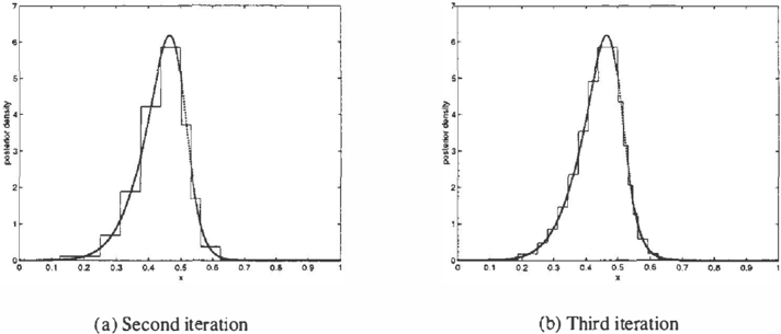
Already on the second iteration, after only one phase of weight propagation, the cliques had a very good estimate of the posterior distribution and therefore the weights. The BSP tree on the second iteration had 1 1 leaves, and the pos­ terior probability distribution differed from the true prob­ ability distribution by a KL distance of 0.03. The BSP tree after the third round of propagation had 1 8 leaves, and the posterior probability distribution differed from the true probability distribution by a KL distance of 0.001 (see Fig. 1 3).

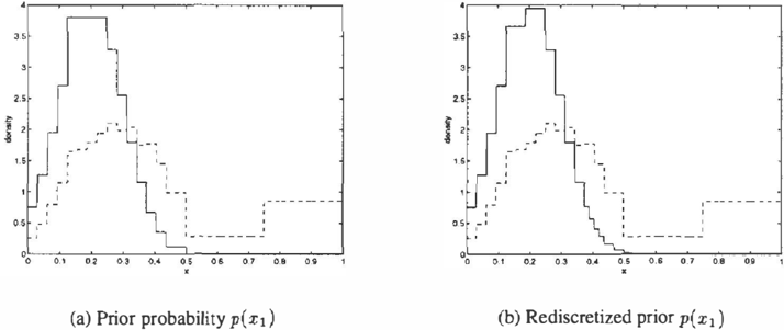
The prior probability discretizations before and after the first weight update are shown in Fig. 14. While at the ini­ tial propagation the N (x1 ; 0.2, 0.01) Gaussian correspond­ ing to the product p(o1 l x 1 )p(x i ) i s discretized with the weight one, the weight is nonuniform for the second round of propagation as shown in Fig. 1 4(b ). The new discretiza­ tion takes into account much larger weights on the right slope and rediscretizes it more finely.

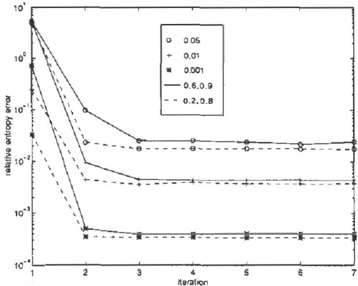
6.2 CONVERGENCE

The algorithm converges by the second iteration in most cases. Figure 15 shows the relative entropy error as a func­ tion of the iteration number for several precision param­ eters 6. The relative entropy error dropped very abruptly after the first iteration and experienced small oscillations around the final answer after that.

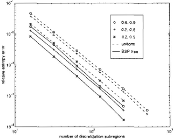
Pruning allows to compare the efficiency of our approach to the uniform discretization. Since we can effectively change discretization focus with evidence, we get a smaller error with our approach than with a uniform approach for the equivalent number of discretization subregions per clique. Figure 16 shows the relative entropy error of a dynamically discretized network compared to a uniformly discretized network given the same number of partitions per clique (so that if we have had N partitions per variable in a uni­ form discretization, we would have N 2 partitions per two­ dimensional clique).

For the nonuniform discretization, we get a factor of 4 bet­ ter precision as compared to the case of uniform discretiza­ tion with the same number of discretization subregions. In practice, the savings can be much bigger since our al­ gorithm can focus the discretization effort on the cliques that have potentials most important for a particular evi­ dence, not potentials of all cliques at the same time. How­ ever, comparison with the uniform discretization is not so straightforward in this case. Although in our simple ex­ periments we did not get any computation time advantage over a uniform discretization-table representation of con­ ditional probabilities is very efficient computationally-we had evidence in Fig. 4 that the nonuniform dynamic dis-

Figure 1 3 : Posterior probability p( x 3 ) for a network shown in Fig. 9 with dynamic discretization for two successive iterations. The result of the inference is shown by a solid line, the exact result is shown by a dotted line. Evidence is o1 = 0.2, o2 = 0.8, and o3 = true.

p( x1 )

p(

)

Figure 14: Original and rediscretized prior probabilities p( x 1 ) . The dashed line shows the estimate of posterior that the clique has after the first weight propagation. Notice the change in the granularity of the discretization. Evidence is 01 = 0.2, 02 = 0.8, and 03 = true.

cretization should be more efficient for more complex do­ mains requiring precision and thus a very fine discretization of multidimensional domains.

7 CONCLUSIONS

In this paper, we provide an effective algorithm for prob­ abilistic inference in hybrid networks with an arbitrary topology and arbitrary functional dependence between variables based on nonuniform dynamic discretization. While our approach is based on discretizing the function, it is derived from the key insight that, within the domain of the function, not all of the regions should be accorded equal importance. We suggest the idea of nonuniform dis­ cretization, which discretizes multidimensional domains as a whole, rather than discretizing each variable separately. Nonuniform discretization has been successfully used in multivariate regression and machine learning. We provide results for the discretization of probability distributions for probabilistic inf erence which show that nonuniform dis­ cretization can be substantially more compact than the tra­ ditional uniform discretization.

Any fixed discretization, however, cannot account well for all possible configurations of evidence. Therefore, we are likely to get large errors for unlikely evidence. We develop a new metric based on the relative entropy that allows to emphasize discretization of some regions as opposed to others and show how to use it in a self-adjusting anytime rediscretization algorithm. This algorithm constantly up­ dates the discretization in accordance with the evidence. It can be run to provide answers of any desired accuracy. Our preliminary empirical results suggest that convergence to the right solution is very rapid in practice.

Given the recent emphasis on building and using hybrid systems, we believe that probabilistic inference algorithms for the corresponding models will become more and more necessary and precision more and more important. As such

,, . .----�-�--�--, number of discretization subregions

systems are typically fairly complex, and involve tightly coupled discrete and continuous elements, exact algorithms are unlikely to be available. Our algorithm deals effectively with arbitrary hybrid systems, so that we can hope that it will be applicable to many of these applications. In partic­ ular, we believe that the ability of our algorithm to adjust itself to the evidence it sees will prove very useful in appli­ cations, e.g., real-time monitoring of hybrid systems, that require fast and efficient change of focus.

Acknowledgments

This research was supported through the generosity of the Powell foundation, by ONR grant N00014-96-l-0718. and by ARO under the MURI program "Integrated Approach to Intelligent Systems", grant number DAAH04-96-1-034l_

References

Alag, S. and A g o g i no , A. M. (1996). Inference using mes­ sage propagation and topology transformation vector gaus­ sian continuous networks. Proceedings o f the T welf th V A/ Conference, pages 20 - 27. Morgan Kaufmann.

Breiman, L., Friedman, J. H., Olshen, R. A., and Stone, C. J. ( 1 984). Classification and regression trees. Wadsworth International Group, Belmont, CA.

Cover, T. a nd Thomas, J. ( 1 99 1 ) . Elements of lnf onnation Theory. John Wiley & Sons, Chichester, UK.

Dechter, R. ( 1 996). Bucket elimination: A unifying frame­ work for probabilistic inference. In Proceedings of the Twelfth V Al Con f erence, pages 21 1 - 219. Morgan Kauf­ mann.

Driver, E. and Morrel, D. (1 995). Implementation of con­ tinuous bayesian networks usi n g sums of weighted gaus­ sians. In Proceedings of the Eleventh VA/ Conf erence, pages 1 34 - 140. Morgan Kaufmann.

Figure 1 6: The relative entropy error as a function of the num­ ber of discretization subregions and evidence. Evidence is 0 1 = 0.6, o2 = 0.9 (circles), o1 = 0.2, 02 = 0.8 (pluses), and 01 = 0.2, 02 = 0.5 (stars). 03 is always true.

Lauritzen, S. L. ( 1 992). Propagation of probabilities, means, and variances in mixed graphical association mod­ els. JASA, 87( 420): 1 089 - 1 108.

Lauritzen, S. L. and Spiegelhalter, D. J. ( 1 988). Local computations with probabilities on graphical structures and their application to expert systems. Journal o f the Royal Statistical Society, B 50:253 - 258.

Lauritzen, S. L. and Wermuth, N. ( 1 989). Graphical mod­ els for association between variables, some of which are qualitative and some quantitative. The Annals o f Statistics, 17( 1 ): 3 1 -57.

Li, Z. and D'Ambrosio, B. ( 1 994 ) . Efficient inference in Bayes networks as a combinatorial optimization problem. International Journal o f Approximate Reasoning, l l ( 1 ):55 - 81 .

Moore, A W. ( 1 99 1 ). Variable resolution dynamic pro­ gramming: Efficiently learning action maps in multivari­ ate real-valued state-spaces. In Machine Learning: Pro­ ceedings o f the Eighth International W orkshop, pages 333 - 337.

Olesen, K. G. ( 1 993). Causal probabilistic networks with both discrete and continuous varibales. IEEE PAM/, 1 5(3):275 - 279.

Pearl, J. ( 1 988). Probabilistic Reasoning in Intelligent Sys­ tems: Networks o f Plausible Inf erence. Morgan Kaufmann.

Samet, H. and Webber, R. ( 1 988). Hierarchical data struc­ tures and algorithms for computer graphics. 1. Fundamen­ tals. IEEE Computer Graphics and Applications, 8(3):48 68.

Wellman, M. P. and Liu. C.-L. ( 1 994). State-space abstrac­ tion for anytime evaluation of probabilistic networks. In Proceedings o f the T enth VA/ Conference, pages 567 - 574. Morgan Kaufmann.