On the Semi-Markov Equivalence of Causal Models

Benoit Desjardins

University of Pittsburgh benoit@med. pitt. edu

Abstract

The variability of structure in a finite Markov equivalence class of causally sufficient mod­ els represented by directed acyclic graphs has been fully characterized. Without causal suf­ ficiency, an infinite semi-Markov equivalence class of models has only been characterized by the fact that each model in the equiva­ lence class entails the same marginal statis­ tical dependencies. In this paper, we study the variability of structure of causal models within a semi-Markov equivalence class and propose a systematic approach to construct models entailing any specific marginal statis­ tical dependencies.

discover the causal structure in a body of data, given certain hypotheses [2, 5, 6, 9, 12, 14]. Graph the­ ory [17] has now emerged as a mathematical language for causality. Graphs provide a strong notational sys­ tem for concepts and relationships not easily expressed by equations and probabilities, and there has been an increased understanding of the fundamental relation­ ships between graphs, causality, and probability.

Key words: causal modeling, latent variables, semi­ Markov equivalence.

1 Introduction

One of the most central problems in scientific research is the search for explanations to some aspect of nature. This often involves a cycle of data gathering, theo­ rizing, and experimentation. In many scientific fields data comes in the form of statistical distribution infor­ mation, representing the value of different features for a sample in a population. One of the tasks in research is to discover some structure in that data. In partic­ ular, one is interested in finding something about the causal processes explaining the statistical data, in the form of a theory or a model of the aspect of nature under study. Such causal model can then be used as a basis for explanation and experimentation.

Although traditional statistical approaches are excel­ lent for finding statistical dependencies in a body of data, they prove inadequate at finding the causal structure in the data [8, 11]. New graphical algorith­ mic approaches have been proposed to automatically

Constraint-based approaches [ 9 , 14] use the condi­ tional independence relations present in a body of statistical data to graphically infer the causal struc­ ture present in the data. Based on strong connections between graph theoretic properties and statistical as­ pects of causal influences, fundamental assumptions about the data ( the Markov condition and the faithful­ ness condition ) are used to infer a graphical structure, which represents statistical dependency relations on a set of variables. Such ( marginal ) dependency graph is used to construct models describing the exact causal relations in the data. Since causal relations cannot be inferred from statistical data alone, a marginal depen­ dency graph is entailed by a possibly infinite equiv­ alence class of models representing competing causal alternatives.

Under the assumption of causal sufficiency, there is a one to one correspondence between statistical depen­ dency and direct causal relation. Two causal mod­ els without latents which entail the same statistical dependencies are called ( local ) Markov equivalent. Every Markov equivalence class of models is finite, and the variability of structure of models within the same Markov equivalence class is very limited. Indeed any two Markov equivalent causal models always share the same causal connections between their variables, but the direction of the causal influences can vary [1, 7, 16] .

If the data contains correlated errors, the assumption of causal sufficiency fails, and latent variables must be introduced in models to explain the causal structure in the data [13]. Two causal models with latent variables which entail the same marginal dependencies are called

semi-Markov equivalent. However marginal statis­ tical dependency does not entail direct causal connec­ tion. Given a model M with latent variables, the set of competing semi-Markov equivalent alternatives is not only large, it is infinite. One can indeed always add new latent variables to a model without chang­ ing the pattern of statistical dependencies between the measured variables. Although there is a well defined test to determine the semi-Markov equivalence of two causal models with latent variables (they must entail the same marginal dependency graph) (14, 15], there is currently no systematic approach for exploring the variability of structure within a semi-Markov equiva­ lence class of causal models.

In this paper, given an infinite semi-Markov equiva­ lence class of models entailing a marginal dependency graph G, we present a finite subset of that class which captures the essential variability of causal structure within the equivalence class, and offer graphical rules for systematically constructing from G any model in that finite subset. After demonstrating that current attempts at generating semi-Markov equivalent alter­ natives to any given model using local graphical trans­ formation rules are too limited, we show that our graphical rules can also be used for that purpose.

2 Formal preliminaries

Causal models are best represented by graphs. We first introduce all the important graph theoretical elements required in this paper (14, 17]. We assume that the reader is already familiar with the very basic concepts from graph theory.

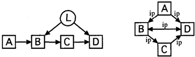
A directed acyclic graph (DAG) is a pair (V, E) such that V is a non empty finite set of elements called vertices (or variables), E is a finite set of ordered pairs of elements of V called edges, and in which there are no cycles. If (V1, V2) E E, then there is an edge from V1 into V2, represented as V1 -+ V2. Figure 1 (left) shows an example of such a DAG. � y conven­ tion latent variables are represented by cucles, and obs � rvables by squares. A causal graph is a directed acyclic graph in which for each (V1, V2) E E, V1 is a direct cause of V2. A causal model is a structure M =< G, P >,where G is a causal graph over a set of variables V, and P is a probability distribution over V. We often identify causal models with their causal graphs in situations not involving P specifically.

The expression I(A, C, B) represents the conditional independence relation of variable A and B given the variables in set C. A causal model < G, P > satis­ fies the Markov condition if every variable in G is conditionally independent of its non-parents and non­ descendants given its parents. < G, P > satisfies the faithfulness condition if all and only the conditional independence relations true in P are entailed by the Markov condition applied to< G, P >.

A collider on a path U is a variable V (excluding the endpoints of U) receiving causal edges from both its two adjacent variables on U (-+ V f-). In a causal graph, two different variables vl and v2 are d-separated given a set of (other) variables W if and only if there is no undirected path u between vl and v2 such that every collider on u has a descendent in W and no other variable on U is in W. They are d­ connected if and only if they are not d-separated. An important theorem is: in a causal model M, if variables vl and v2 are d-separated given a set of variables w then I(V1, W, V2) (9].

An inducing path (relative to a set S of variables) from variable vl to variable v2 in a causal graph is a path U from V1 into V2 (V1 . . . -+V2, V1 # V2) such that every variable in S \ { V1 , V2} is a collider on U, and every collider on u is an ancestor of either vl or v2. There is an inducing path from variable V1 to variable V2 if and only if V1 and V2 are not d-separated given any subset of S \ {V1, V2}. An inducing path represents a statistical dependency implied by a causal model on a marginal distribution.

The inducing path graph (IPG) entailed by a causal model M relative to a subset S of the varial;>les in M is a DAG with two kinds of edges: (1) V1 � V2, in­ dicating that there is an inducing path in M relative to S between V1 and V2 into V2, but not into Vt, and (2) V1 � V2, indicating that the inducing path is also into V1 (Figure 1 right). The lPG of a model M re � re­ sents all the dependencies implied by M on a margmal distribution over a subset S of its variables (S usually corresponds to the set of observables in M). From each model M one can compute the corresponding induc­ ing path graph IPG(M), by determining the induc­ ing paths in M between its observable variables. The IPGs of any two semi-Markov equivalent causal mod­ els share the same adjacencies, but might not share the same edge orientations. The marginal depen­ dency graph (MDG) entailed by a causal model M (also called partially oriented lPG (POIPG) or par­ tial ancestral graph (PAG)), is a graph which has the

same adjacencies as IP G ( M ) , but contains only edge orientations that are common to the IPGs of all mod­ els semi-Markov equivalent toM. Missing orientations are indicated by small circles.

3 Variability of causal models

Current constraint-based causal model discovery algo­ rithms do not discover causal models from data. They rather discover marginal dependency graphs [14], rep­ resenting an infinite equivalence class of semi-Markov equivalent causal models. We seek to study the vari­ ability of structure of models in that equivalence class, and to offer an approach to construct these models.

A marginal dependency graph G represents a finite set S of semi-Markov equivalent IPGs entailing G, and contains only edge orientations that are common to all the IPGs in S. A semi-Markov equivalence class of models can thus be finitely partitioned into infinite subclasses of models, the models within each subclass entailing the same IPG. Each IPG inS is a completion of G. Any completion of G must obey certain rules to represent an IPG: it must be acyclic, and must respect certain internal consistency rules, indicated in the fol­ lowing theorem ( proved in appendix ) :

Theorem 1 Let G be an acyclic graph with !.!+ edges and � edges. Let RI be the following rule: if in G . � � there zs an edge A -=t B and an edge B f+ C and B is an ancestor of C in G, then there must be an edge A � C in G. RI must hold in all IPGs. Let R2 be the following rule: if in G there is a path of � edges between variables A and B, and every variable on that path is an ancestor of A or B, then there must be an edge A � B in G. R2 must hold in all IPGs. An extended DAG containing � edges is an IPG if and only if it is closed under the set of rules {RI, R2}.

Given a marginal dependency graph G, the finite set of all of its acyclic completions closed under rules RI and R2 is the set of all semi-Markov equivalent IPGs entail­ ing G. Without causal sufficiency, any given IPG Gi is entailed by an infinite set Si of semi-Markov equiva­ lent causal models. We seek to identify a finite subset of Si capturing the essential variability of causal struc­ ture in Si by expanding Pearl's [9] notion of "minimal models" to models with latent variables.

3.1 Minimal models

In [9], Pearl intuitively defines a causally sufficient minimal model as a graph in which every proper sub­ graph does not satisfy the Markov condition. We now extend this definition to models with latents [3].

Let SI be the set of all DAGs. Let M be in SI. Let e be in E, the set of all edges of M. Let VI , v2 be in V, the set of all vertices of M. The operator REe () : S I --+ S 1 is defined such that REe(M) is the same DAG as M, but with edge e removed. The operator CVv1,v2 () : SI --+ S I is defined such that CV v1,v2 ( M ) is the same DAG as M, but with variable v2 substituted for VI in all edges of M, and all self-pointing edges removed. Thus VI and v2 become collapsed in the new DAG. RE stands for "remove edge" and CV for "collapse variables" .

Let M be a model. Let OI be the set of all possible operators REe(), where e is an edge in M. Let 02 be the set of all possible operators CV v1 ,v2 () , where VI and v2 are distinct variables in M. A reducing transformation R is a finite composition of operators in OI U 02. If there is a reducing transformation R such that IPG(R(M)) = IPG(M), then the model R( M ) is a reduction of M. The model is minimal ( or irreducible ) if for every reduction R(M) of M, we have R(M) = M.

In other words, a minimal model is a model in which it is not possible to remove an edge or to collapse two variables in its graph without always ending up with a new model which has a different inducing path graph. Although minimal models are defined in terms of in­ ducing path graphs for practical reasons, this turns out to be equivalent to a definition using conditional inde­ pendence relations ( as in the causally sufficient case ) if only latent variables are allowed to be collapsed.

An edge in a causal model M is an essential edge if it cannot be removed without changing the induc­ ing path structure of M. Minimal models have only essential edges, and are the simplest models satisfying a causal theory. Minimal models do not imply simple models, but rather simplest models. They can be quite complex and contain many latent variables, including embedded and causally related latents. The essential variability of an infinite set of semi-Markov equivalent causal models is fully captured by its finite subset of minimal models [4], although a formal proof of this fact is beyond the scope of this paper.

3.2 Constructing causal models

We now clarify the relation between IPGs and causal models. Consider a causal model M over the set V of variables { V1 , ... , Vn}. The IPG of M over the sub­ set V' of the observable variables in V is a graph G with variables V'. In G, if there is a directed edge A � B, then either A is a direct cause of B, or there is an indirect inducing path between A and B in M. As a reminder, an inducing path between A and B relative to V' is a path U from A into B involving a

combination of variables in V' (observables) and vari­ ables in V" = V \ V' (latents). Variables in V' on U must all be colliders and ancestors of A or B. Vari­ ables in V" on U can be pretty much anything, but if they are colliders, they must be ancestors of A or B. So the causal relations between observable variables in the causal model are strongly determined by the edges in the lPG, while the causal relations involving latent variables are not as constrained. In G, if there is a bidirected edge A � B, then by acyclicity, there must be a latent common cause T between A and B. This might be a direct common cause, or a common cause of some other pair of variables (that could include A or B), which spreads to A and B through the structure of the inducing paths.

Let G be an lPG. We show that each model M in the set of semi-Markov equivalent minimal models entail­ ing G is a systematic graphical transformation of G.

An expansion M; of IPG G is a graphical transforma­ tion of G made by replacing in G every edge of the form iP. A --'+ B by the causal edge A --+ B, and every edge of iP. the form A ABby a latent path A f-LAB --+ B, possibly combined with a hidden edge A --+ B or B --+ A (making sure the hidden edge does not create new in­ ducing paths or cycles). Each M; is a causal model entailing G and is uniquely determined by the choice of hidden edges in G.

Graphical operators RE() and CV() have already been defined. We now define two additional operators. First, the operator ELv,,v,,v,,l, () : S1 --+ S1 is defined such that ELv,, v2,v3, z , (M) has the same causal graph as M, but if there is a pattern [ v1 --+ v2, l1 --+ v2, l1 --+ v3] in the model where l1 is a latent variable and v1, v2 and v3 are observable variables, it is replaced by the pattern [v1--+ l1,h--+ v2,h--+ vs,l2--+ v2,l2--+ v3], where l2 is a new latent. Second, the operator CLz,,t,,v() : S1--+ S1 is defined such that CLt,,z,,v(M) has the same causal graph as M, but if there is a pat­ tern ll1 --+ v, l2 --+ v] in the model where h and l2 are latent variables and v is an observable variable, it is replaced by the pattern [l1 --+ l2, l2 --+ v]. The first operator produces embedded latents (EL stands for "embed latent"), while the second produces causally connected latents ( CL stands for "connect I a tents"). Note that the EL() operator introduces a new latent, because of the fact that minimal models with embed­ ded latents can have in some rare cases more latent variables than the number of � edges in the lPG [4]. In most cases in practice, a simpler version EL*() is used, which does not introduce a new latent. We now have the following important theorem (the algorithm is sketched in appendix, and the full proof can be found in [4]): ·

Theorem 2 Let G be an IPG. Every minimal model M; entailing G is a well defined graphical transforma­ tion of an expansion of G using operators RE, CV, ELand CL.

We not only have the tools to construct a minimal model entailing a given marginal dependency graph, but we have the tools to construct all such minimal models. The computational complexity of minimal model construction is on average O(n 3 ) per model, where n is the number of variables in the marginal dependency graph [4]. Given a marginal dependency graph G, the number of minimal models entailing G increases exponentially with the number of edges in G, and strongly depends on the number of missing orien­ tations in G. For marginal dependency graphs with many missing orientations, one can most efficiently constrain the set of IPGs (and therefore the number of minimal models) by using background know ledge on the observable variables.

4 Constructing equivalent alternatives

In the causally sufficient case, it has been formally demonstrated that any model Markov equivalent to some model M can be constructed from M by a se­ quence of edge reversal operations using only local constraints [1, 7, 16]. A natural approach with semi­ Markov equivalent models is to extend this set of local graphical rules to take into account latent variables. This is what Pearl attempts in [10]. In this paper, Pearl uses B edges in causal graphs to indicate corre­ lated errors between two variables. He then proposes two graphical transformation rules to construct linear semi-Markov equivalent models:

Rule 1: X --+ Y is interchangeable with X B Y if every neighbor (variable connected by a B edge) or parent of X is adjacent to Y.

Rule 2: X --+ Y can be reversed into X f- Y if every neighbor or parent of Y (excluding X) is adjacent to X, and every neighbor or parent of X is adjacent to Y.

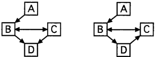
These rules are unfortunately flawed (for both general· models and linear models). Let M be a causal model, in which every latent variable has no parent and is the common parent of two observable variables. In such models, subpaths A tL --+ B can be replaced by edges A B B, representing correlated errors. Pearl uses such models with B edges in his study of semi­ Markov equivalence. We now include a counterexam­ ple to Pearl's rule 2. A counterexample to Pearl's rule 1 can be easily produced using the same principles. Consider the following causal model M1 of Figure 2, where B B C indicates a correlated error between B

and C. In this specific case, this also corresponds to a hidden common latent cause of B and C.

According to Pearl's rule 2, the edge C-+ D can be re­ versed into C +-D to produce semi-Markov equivalent model M2, since the parent B of D is adjacent to C, and the neighbor B of C is adjacent to D. But M2 is not semi-Markov equivalent to M1. Indeed since B is an ancestor of C in M2, there is now an inducing path from A to C in M2, which is not present in M1. Since M1 and M2 do not entail IPGs of same adjacencies, they cannot be semi-Markov equivalent.

Pearl's rules may be flawed, but they can be trans­ formed into more specialized rules, which are not flawed.

Rule 1': X -+ Y is interchangeable with X f+ Y if every neighbor of X is a neighbor of Y, and every parent of X is a parent of Y.

Rule 2': X -+ Y can be reversed into X f- Y if every neighbor of Y is a child of X, every neighbor of X is a child of Y, and every parent of X is a parent of Y.

These rules are sufficient, but neither is necessary. This set can be complemented by many additional suf­ ficient and specialized rules. Such large sets of special­ ized sufficient rules enable the construction of a hand­ ful of models semi-Markov equivalents to any given model. But this approach fails to consider the exten­ sive variability of graphical structure in sets of semi­ Markov equivalent causal models.

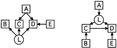
Consider the two models in Figure 3, which are semi­ Markov equivalent. M1 contains a latent common

cause of three different observable variables, while M2 contains an embedded latent. In M2, observables B and D are neither connected directly nor through a common latent. One cannot construct M2 from M1 using simple edge replacement or edge reversal oper­ ations. Any single edge transformational approach to generating semi-Markov equivalent causal models is thus too limited. A larger and more powerful set of graphical operators is required. The set of operators proposed in the previous section turns out to be suffi­ cient for that purpose. We now offer an approach to generate models semi-Markov equivalent to any model M by first determining the marginal dependency graph of M, and then constructing minimal models entailing the same marginal dependency graph.

In [14, 15], it is formally demonstrated that two causal models with latent variables are semi-Markov equiva­ lent if and only if they entail the same marginal de­ pendency graph. In order to find models semi-Markov equivalent to some causal model M, we first extract from M it's marginal dependency graph. This is a two step process: (1) determine the lPG forM, and (2) ex­ tract the marginal dependency graph of this lPG. The first step is a well defined graphical transformation of M. The second step is unfortunately an open prob­ lem, which we do not attempt to solve in this paper. Instead, we use a modified version of the TETRAD al­ gorithm of Spirtes, et al. [14] to reconstruct it in three steps: (1) remove all edge orientations from the lPG, (2) let A, B and C be any triple of vertices such that A is adjacent to B and B is adjacent to C, but A is not adjacent to C in the lPG; if there is no set Z of observ­ able variables in M such that A and C are d-separated by B U Z, then make B a collider between A and C, otherwise make B a definite non-collider between A and C, and (3) use the TETRAD orientation rules to determine as many missing orientations as possible. The problem is open because it is not formally proven that TETRAD's set of orientation rules is complete.

Once the marginal dependency graph G is determined, it suffices to use the already introduced graphical ma­ chinery to generate any causal model entailing G. All such models are semi-Markov equivalent toM.

4.1 Example

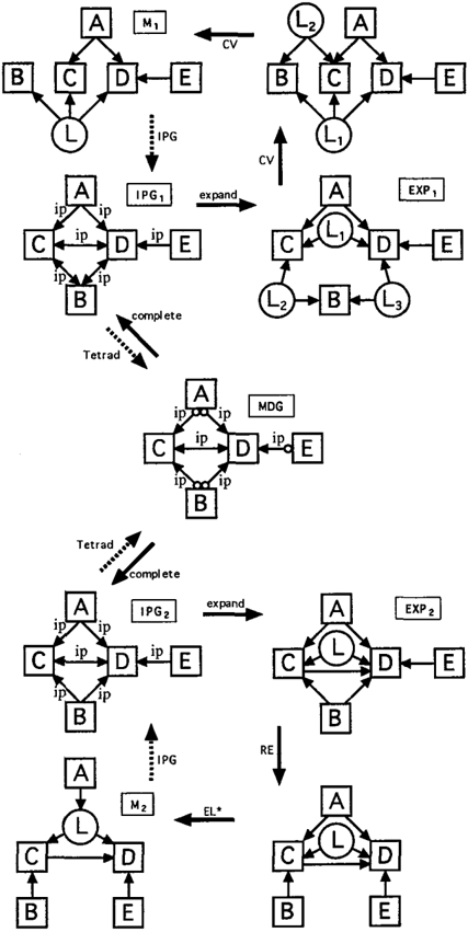
Figure 4 illustrates how the two semi-Markov equiva­ lent minimal models of Figure 3 are constructed from their common marginal dependency graph (MDG): two self-consistent semi-Markov equivalent inducing path graphs are constructed (IPG1 and IPG2), by performing different completions of the missing orien­ tations (small circles). The non minimal expansions EX Pt and EX P2 are then produced from the respec­ tive inducing path graphs by replacing correlated er-

：

rors by common latents causes and choosing which hid­ den causal edges to include: no hidden causal edge for EXP1 and hidden edge C--+ D for EXP2. Note that a hidden edge D --+ C would not be allowed in EX P2, as it would entail the inducing path E $. C, which is not present in I P G2. Then M1 is constructed from EX P1 by collapsing its three latents into a single la­ tent L, and M2 is constructed from EX P2 by remov­ ing the non essential causal edge B --+ D ( since the path B --+ C tL --+ D generates the inducing path B $.D) and embedding L between A, C and D.

To perform the inverse operation (dotted arrows ) and construct the marginal dependency graph from each minimal model, it suffices to compute the inducing path graph for each model, and then use the Tetrad algorithm to compute their common marginal depen­ dency graph.

The same example is used to illustrate how to con­ struct semi-Markov equivalent alternatives to any given model: by first determining the marginal de­ pendency graph, and then making choices of missing orientations and hidden edges to produce IPG expan­ sions, which are then reduced by graphical transfor­ mations to produ.ce different minimal models. There are obviously finitely many different IPG expansions produced from a marginal dependency graph. It is formally demonstrated in [4) that the total number of semi-Markov equivalent minimal models entailing a marginal dependency graph is also finite. The en­ tire set of such minimal models can be efficiently con­ structed using our approach, whose main computa­ tional advantage is the important restriction of the search space of models.

5 Conclusion

These results are part of a larger study on the theoret­ ical limits to reliable causal inference [ 4). Constraint­ based causal models discovery algorithms determine marginal dependency relations between variables, and implicitly represent sets of semi-Markov equivalent models by a single graphical structure. In this paper, we provided the formal tools to generate causal mod­ els entailing this graphical structure. Neither Markov equivalence nor semi-Markov equivalence entail distri­ bution equivalence. By explicitly capturing the essen­ tial variability of graphical structure within a semi­ Markov equivalence class of models, insights can be obtained about the formal properties of these mod­ els, and methods can be proposed to experimentally or observationally discriminate between non distribu­ tion equivalent models within the same semi-Markov equivalence class [4).

These results have also practical usefulness. Using our approach, a researcher using causal models can now, given any model satisfying a body of statistical data over a set of observable variables, automatically and systematically generate any simple alternative model explaining the data. Such alternatives might prove a valuable source of explanatory insight.

6 Appendix: Proofs

Theorem 1 Let G be an acyclic graph with $ edges and � edges. Let R1 be the following rule: if in G there is an edge A $ B and an edge B � C and B is an ancestor of C in G, then there must be an edge A $ C in G. R1 must hold in all IPGs. Let R2 be the following rule: if in G there is a path of � edges between variables A and B, and every variable on that path is an ancestor of A orB, then there must be an edge A � B in G. R2 must hold in all IPGs. An extended DA G containing � edges is an IPG if and only if it is closed under the set of rules {R1, R2}.

To prove the theorem, we first prove this short lemma:

Lemma 3 Let M be a causal model with IPG G. If there is a directed path from variable A to variable B in G, then A is an ancestor of B in M.

· iP. iP. iP. Proof: Let U be the directed path A -=+ V1 -=+ . . . -=+ Vn $ B in G. Each inducing path Vk $ Vk+l in G corresponds to a path Uk in M that is out of Vk, and in which every collider is an ancestor of either Vk or Vk+l· Let Wk be the first collider on Uk starting at Vk. By acyclicity Wk must be an ancestor of Vk+l and not of Vk. Therefore Vk must be an ancestor of Vk+l in M. Since this applies to every edge on U, then A must be an ancestor of B in M. 0

The theorem can now be proven.

iP. Proof: Assume M entails IPG G. An edge A -=+ B in G implies that there is an inducing path U1 from A into B in M, and by the previous lemma that A is an ancestor of B in M. An edge B � C in G implies that there is an inducing path U2 between A and B into both B and C in M. By concatenating the two paths U1 and U2 at B into a new path U, B becomes a collider on U, and is an ancestor of C. Thus U is an inducing path from A into C. So R1 holds in every iP. iP. iP. iP. IPG. Let A B vl B . . . B Vn B B be a path between A and B in G, with each Vk ancestor of A or B ( by convention A and B are ancestors of themselves ) . The edge Vk � Vk+1 in G implies that there is an induc­ ing path uk between vk and vk+l into both vk and Vk+l in M, with every collider being an ancestor of Vk or Vk+l, and therefore of A or B by hypothesis. The concatenation of all these Uk creates a path in which every observable is a collider, and every collider is an ancestor of either A or B, thus an inducing path into A and into B. So R2 holds in every IPG. Closure un­ der R1 and R2 is therefore necessary in an IPG. Since any observable in an inducing path ( except the end­ points ) must be a collider, the only other combination of inducing paths not already covered that creates a new inducing path is A $ V1 � . . . � Vn � B, with each Vk ancestor of A or B, which implies the inducing path A .$ B. But by acyclicity V1 is necessarily ancestor of B, thus each Vk is ancestor of B, which implies by R2 the path V1 � B. But then R1 with A$ V1 � B implies A$ B. Thus closure under R1 and R2 is sufficient. 0

Theorem 2 Let G be an IPG. Every minimal model M; entailing G is a well defined graphical transforma­ tion of an expansion of G using operators RE , CV , ELand CL .

Here we only provide a sketch of the model construc­ tion algorithm. The full detailed proof, which is quite long and involves the reverse construction of minimal models of decreasing complexity, can be found in (4].

Proof: Given an expansion of G, the following sets of minimal models of increasing complexity are sequen­ tially generated: those involving only external latents, those also involving embedded latents, and those also involving connected latents. All generated models en­ tail the same IPG G.

First, given an expansion M1 of G, all non essential edges A -+ B (A, B observables ) are removed from M1 to produce model M2 entailing the same IPG G. A non essential edge A-+ B is easily identified in M1 by a simple graphical rule ( lemma 4), and removing any such non essential edge from M1 does not make an initially non essential edge become essential. Hidden edges are treated as special edges in the processing. The next step is to remove all non-essential latents L from M2 ( equivalent to removing two non-essential edges per latent ) to produce model M3 entailing the same IPG. All non essential latents in M2 are identified using simple graphical rules. Unfortunately removing a non-essential latent L can occasionally make some other non-essential latent L' become essential. The order of removal of non-essential latents is therefore important, and M3 is usually not unique, but rather represents a very small set of alternatives.

Next, for each model M3, collapsibility of latents is as­ sessed using simple graphical rules, and latents are col­ lapsed to produce minimal model M4. Unfortunately, collapsing two latents can make two initially collapsi­ ble latents become non-collapsible. The order of col­ lapsibility is therefore important, and M4 is again not unique, but represents a finite set of alternatives. The entire set of minimal models with external latents is generated using the previous few steps.

Next, for each model M4, embeddability of latents is assessed using simple graphical rules, and latents are embedded to produce minimal model M5. Many com­ bination of embeddings can be performed, with the result still being a minimal model. Thus M5 is not unique. This generates the entire set of minimal mod­ els with embedded latents entailing the same lPG.

Finally, for each model M5, connectibility of latents is assessed using simple graphical rules, and latents are connected to produce minimal model M6· Many combination of latent connections can be performed, with the net result still being a minimal model. Thus M6 is not unique. But this generates the entire set of minimal models entailing the same lPG. 0

In the algorithm, simple graphical rules are used to as­ sess features of variables or edges. Most of the power of the algorithm comes from the simplicity of such rules. Here as an example is the rule for determining the non­ essentiality of edges in M1. A complete description of the other rules can be found in [4]

Lemma 4 Let E = A -+ B be a non hidden edge in the expansion M1 of IPG G. E is non essential {in all models of G) if and only if there is a path U1 A-+ C +-L-+ B in M1 with C ancestor of B.

Proof: Assume there is such a path U1 in G1. U1 is an inducing path from A into B in M1 not involving E, so E is non essential. For the converse, assume that E is non essential. Then there must be an inducing path U between A and B into B in M1. Then U starts with A -+ C for some observable C and continues with alternating latent common causes and observable col­ liders. Since by acyclicity C cannot be an ancestor of A, it is an ancestor of B. Every collider on U is an ancestor of A or B, thus every collider is an ancestor of C or B and therefore of B. This implies the ex­ istence of an inducing path between C and B that is into both C and B. Thus there is a C � B edge in G and therefore there is an A -+ C +-L -+ B path in M1, with C ancestor of B. 0

References

1. Chickering DM: A transformational character­ ization of Bayesian network structures. In P. Besnard and S. Hanks (Eds.), Uncertainty in AI 11, Morgan Kaufmann, San Francisco, CA, 87-98, 1995.
2. Cooper, GF, Herskovits E: A Bayesian method for the induction of probabilistic networks from data. Machine Learning 9, 1992, pp 309-347.
3. Desjardins B: Equivalence of causal theories. lOth Internat Congr of Logic, Methodology, and Phi­ losophy of Science, Florence, Italy, August 1995.
4. Desjardins B: On the theoretical limits to reliable causal inference. PhD dissertation, University of Pittsburgh, 1998.
5. Glymour C, Scheines R, Spirtes P, Kelly K: Dis­ covering causal structure. Academic Press, New York, 1987.
6. Beckerman D, Geiger D, Chickering, D: Learning Bayesian networks: The combination of knowl­ edge and statistical data. Machine Learning 20, 1995, pp 197-243.
7. Meek C: Causal inference and causal explanation with background knowledge. In P. Besnard and S. Hanks (Eds.), Uncertainty in AI 11, Morgan Kaufmann, San Francisco, CA, 403-410, 1995.
8. Mosteller F, Tukey J: Data analysis and regres­ sion, A second course in regression. Addison­ Wesley, Massachusetts, 1977.
9. Pearl J: Probabilistic reasoning in intelligent sys­ tems. Morgan Kauffman, San Mateo CA, 1988.
10. Pearl J: Graphs, Causality and Structural Equa­ tion Models, Technical Report (R-253), UCLA Cognitive Systems Laboratory, August 1997. Pre­ pared for Sociological Methods and Research, Special Issue on Causality.
11. Rawlings J: Applied regression analysis. Wadsworth, Belmont, CA, 1988.
12. Schacter R: Evaluating influence diagrams. Oper­ ations Research, 34(6), 1986.
13. Spirtes P: Building causal graphs from statisti­ cal data in the presence of latent variables. In B Skyrms (ed), Proc IX Intern Congr on Logic, Methodology and Philosophy of Science, Uppsala, Sweden, 1991.
14. Spirtes P, Glymour C, Scheines R: Causation , Prediction, and Search. Springer-Verlag, New York, 1993.
15. Spirtes P, Verma T: Equivalence of causal mod­ els with latent variables. Technical Report CMU­ Phil-33, June 1994.
16. Verma T, Pearl J: Equivalence and synthesis of causal models. Proc Sixth conf on Uncertainty in AI, Mountain View, CA, pp 220-227, 1991.
17. Wilson RJ: Introduction to graph theory. Long­ man, Essex, England, 1985.