On the Testable Implications of Causal Models with Hidden Variables

Jin Tian and Judea Pearl

Cognitive Systems Laboratory

Computer Science Department

University of California, Los Angeles, CA 90024 {jtian, judea } @cs. ucla. edu

Abstract

The validity of a causal model can be tested only if the model imposes constraints on the probability distribution that governs the gen­ erated data. In the presence of unmeasured variables, causal models may impose two types of constraints: conditional independen­ cies, as read through the d-separation crite­ rion, and functional constraints, for which no general criterion is available. This paper of­ fers a systematic way of identifying functional constraints and, thus, facilitates the task of testing causal models as well as inferring such models from data.

1 Introduction

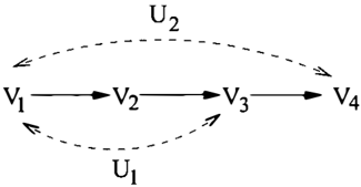
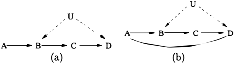
It is known that the statistical information encoded in a Bayesian network (also known as a causal model) is completely captured by conditional independence relationships among the variables when all variables are observable [Pearl et al., 1990]. However, when a Bayesian network invokes unobserved variables, or hidden variables, the network structure may impose equality and inequality constraints on the distribu­ tion of the observed variables, and those constraints may not be expressed as conditional independencies [Spirtes et al., 1993, Pearl, 1995]. Verma and Pearl (1990) gave an example of non-independence equality constraints shown in Figure 1 (a), in which U is un­ observed. 1 A simple analysis shows that the quantity l:b P(dla, b, c)P(bla) is not a function of a, i.e.,

This constraint holds even though no restrictions are made on the domains of the variables involved and on

1 We use dashed arrows for edges connected to hidden variables.

the class of distributions involved. This paper develops a systematic way of finding such functional constraints.

Finding non-independence constraints is useful both for empirically validating causal models and for distin­ guishing causal models with the same set of conditional independence relationships among the observed vari­ ables. For example, the two networks in Figure 1 (a) and (b) encode the same set of independence state­ ments (A is independent of C given B), but they are empirically distinguishable due to Verma's constraint (1). A structure-learning algorithm driven by condi­ tional independence relationiships would not be able to distinguish between the two models unless the con­ straint stated in Eq. (1) is tested and incorporated into the model-selection strategy.

Algebraic methods for finding equality and in­ equality constraints implied by Bayesian networks with hidden variables have been presented in [Geiger and Meek, 1998, Geiger and Meek, 1999]. However, due to high computational demand, those methods are limited to small networks with small number of probabilistic parameters. This paper deals with conditional independence constraints and functional constraints, the type of constraints imposed by a network structure alone, regardless the domains of the variables and the class of distributions. The conditional independence constraints can be read via the d-separation criterion [Pearl, 1988], but there is no general graphical criterion avail­ able for Verma type functional constraints that are not captured by conditional independencies

[ Robins and Wasserman, 1997, Desjardins, 1999]. This paper shows how the observed distribution factorizes according to the network structure, estab­ lishes relationships between this factorization and Verma-type constraints, and presents a procedure that systematically finds these constraints.

The paper is organized as follows. Section 2 intro­ duces Bayesian networks and shows how functional constraints emerge in the presence of hidden variables. Section 3 shows how the observed distribution factor­ izes according to the network structure and introduces the concept of c-component, which plays a key role in identifying constraints. Section 4 presents a procedure for systematically identifying constraints. Section 5 shows that, for the purpose of finding constraints, in­ stead of dealing with models with arbitrary hidden variables, we can work with a simplified model in which each hidden variable is a root node with two observed children. Section 6 concludes the paper.

2 Bayesian Networks with Hidden Variables

A Bayesian network is a directed acyclic graph ( DAG ) G that encodes a joint probability distribution over a set V = {V1, ... , V n} of random variables with each node of the graph G representing a variable in V. The arrows of G represent probabilistic dependencies be­ tween the corresponding variables, and the missing arrows represent conditional independence assertions: Each variable is independent of all its non-descendants given its direct parents in the graph. 2 A Bayesian network is quantified by a set of conditional probabil­ ity distributions, P( v; I Pa i ), one for each node-parents family, where P A; denotes the set of parents of v;, and v; and pa; denote an instantiation of values of v; and P A; respectively. 3 The assumptions encoded in the network amount to asserting that the joint probability function P( v) = P( v1, ... , v n) factorizes according to the product [ Pearl, 19 88 ] :

When some variables in a Bayesian network are unob­ served, the marginal distribution of observed variables can no longer factorize according to Eq. (2). Letting

2 We use family relationships such as "parents," "chil­ dren," "ancestors," and "descendants," to describe the ob­ vious graphical relationships. For example, we say that v; is a parent of V; if there is an arrow from node v; to V;, Vi-tV;.

3We use uppercase letters to represent variables or sets of variables, and use corresponding lowercase letters to rep­ resent their values (instantiations).

V = {V1, ... , V n} and U = {U1, ... , Un'} stand for the sets of observed and hidden variables respectively, the observed probability distribution, P( v), becomes a mixture of products:

where P Av, and P A u , stand for the sets of parents of v; and U; respectively, and the summation ranges over all the U variables. Since all the factors of non­ ancestors of V can be summed out from Eq. (3), letting U' be the set of variables in U that are ancestors of V, Eq. ( 3) then becomes

Therefore, we can remove from the network G all the hidden variables that are not ancestors of any V vari­ ables, and we will assume that each U variable is an ancestor of some V variable.

To illustrate how functional constraints emerge from the factorization of Eq. ( 4), we analyze the example in Figure 1 ( a). For any set S <;:; V, define the quantity Q[S] to denote the following function

In particular, we have Q[V](v) P(v) and, for consistency, we set Q[0](v) = 1, since Lu rr{iiU;EU} P(u;lpau.) = 1. For convenience, we will often write Q[S](v) as Q[S]. For Figure 1 ( a), Eq. (4) becomes

where

From (6), we obtain

and from ( 7),

物 4

=

--;

Eq. (9) implies that Q[{D}] is a function only of c and d, therefore Eq. ( 1 0 ) induces a constraint that the quantity Lb P(dJa, b, c)P(bla) is independent of a.

Note that the key to obtaining this constraint rests with our ability to express Q[{B, D}] and Q[{D}] in terms of observed quantities ( see (8) and (10)), namely quantities not involving U. Applying the same anal­ yses to Figure 1 ( b ) , we have that Q[{D}] gives the same expression as in Eq. (10), but now Q[{D}] = L: u P (dJc, a, u)P(u) is also a function of a, and no Verma constraint is induced. In general, for any set S C V, Q[S] in Eq. (5) is a function of values only of a subset of V. Therefore, whenever Q[S] is computable from the observational distribution P( v), it may lead to some constraints - conditional independence rela­ tions or Verma-type functional constraints. In the rest of the paper, we will show how to systematically find computable Q[S], but first, we study what the argu­ ments of Q[S] are.

For any set C, let Gc denote the subgraph of G com­ posed only of variables in C, let An( C) denote the union of C and the set of ancestors of the variables in C, and let An u (C) = An(C) n U denote the set of hidden variables in An(C). In Eq. (5), the factors corresponding to the hidden variables that are not an­ cestors of Sin the subgraph G suu can be summed out, and letting U(S) = An u (S)asuu be the set of hidden variables that are ancestors of S in the graph G suu, Q[S] can be written as

We see that Q[S] is a function of S, the observed par­ ents of S, and the observed parents of U(S). We will call an observed variable v; an effective parent of an observed variable Vj if v; is a parent of Vj or if there is a directed path from v; to Vj in G such that every internal node on the path is a hidden variable. For any set S<:;;; V , letting Pa+(s) denote the union of S and the set of effective parents of the variables in S, then we have that Q[S] is a function of Pa + (S). Assuming that Q[S] is a function of some set T, when Q[S](t) is computable from P(v), its expression obtained may be a function of values of some set T' larger than T (T C T'), and this will lead to constraints on the dis­ tribution P(v) that the expression obtained for Q[S] is independent of the values t' \ t, which could be a Verma-type functional constraint or be a set of condi­ tional independence statements.

Next we give a lemma that will facilitate the computa­ tion of Q[S] and the proof of other propositions. The lemma provides a condition under which we can com­ pute Q[W] from Q[C], where W is a subset of C, by simply summing Q[C] over the remaining variables ( in C \ W). For any set C, let An·(c) =An( C) n V be the set of observed variables in An( C), and let De·(c) denote the set of observed variables that are in C or are descendants of any variable in C. A set A <:;;; V is called an ancestral set if it contains its own observed ancestors (A = An·(A)), and a set A <:;;; V is called a descendent set if it contains its own observed de­ scendants (A = De·(A)). Letting G(C) = Gcuu(C) denote the subgraph of G composed only of variables inC and U(C) which corresponds to the quantity Q[C] ( see Eq. (11)), then we have the following lemma.

Lemma 1 Let W <:;; C <:;;; V , and W' = C \ W. If W is an ancestral set in G (C) (W = An·(W)a(c ) ), or equivalently, if W' is a descendent set in G ( C) (W' = De·(w')a(c ) ), then

Proof sketch: By Eq. ( 1 1 )

All factors in (13) corresponding to the variables ( ob­ served or hidden ) that are not ancestors of W in G (C) are summed out, and we obtain

We have Anu ( W ) a(C) = An u (W)a wuu = U (W) due to that W is an ancestral set. Therefore the left hand side of (14) is equal to Q[W] by Eq. (11). D

In the next section, we show how the distribution P( v) decomposes according to the network structure and how the decomposition helps the computation of Q[S].

3 C-components

P( v) as a summation of products in ( 4) may sometimes be decomposed into a product of summations. For example, in Figure 2, P(v) can be written as

v4

The importance of this decomposition lies in that both terms Q[{Vi, V 3 }] and Q[{V2, V 4}] are com­ putable from P( v) as shown later. First we study graphical conditions under which this kind of de­ composition is feasible, extending conditions given in [Tian and Pearl, 2002] to the case of non-root U vari­ ables.

Assume that P(v) in Eq. (4) can be decomposed into a product of summations as:

where the variables in S0 have no hidden parents, U is partitioned into Nj 's, and V \ S0 is partitioned into Sj's. U; and Uj must be in the same set Nk if (i) there is an edge between them (U;-+ Uj or U; +-Uj), or (ii) they have a common child (U; -+ U1 +-Uj or U;-+ Vi+Uj) · Repeatedly applying these two rules, we obtain that U; and Uj are in the same set Nk if there exists a path between U; and Uj in G such that (i) every internal node of the path is in U, or (ii) ev­ ery node in V on the path is head-to-head ( -+ Vi+-). It is clear that this relation among U;'s is reflexive, symmetric, and transitive, and therefore it defines a partition of U. We construct S; as follows: a vari­ able V k E V is in S; if it has a hidden parent that is in N;. S;'s form a partition of V \ S0 since N; 's form a partition of U. Let each variable Vi E S0 form a set by itself S? = { Vi }. We have that S;'s and S?'s form a partition of V . It is clear that if a hid­ den variable Uk is not in Nj, then it does not appear in the factors of IT v, ES; P( v; IPavJ ITu, EN; P( u; lpa.,;), hence the decomposition of P(v) in Eq. (16) follows. We will call each S; or S? a c-component (abbrevi­ ating "confounded component") of V in G or simply c-component of G . This definition of c-component reduces to that introduced in [Tian and Pearl, 2002] in the special case of all hidden variables being root nodes.

Assuming that V is partitioned into c-components

S1, ... , Sk, Eq. (16) can be rewritten as

which follows from

where we have used the following formula

We will call Q[S;] the c-factor corresponding to the c­ component S;. For example, Figure I (a) is partitioned into c-components {A}, {C}, and {B,D}, with corre­ sponding c-factors Q[{A}] = P(a), Q[{C}] = P(clb), and Q[{B,D}] in (7) respectively, and P(v) can be written as a product of c-factors as in Eq. (6). In Figure 2, V is partitioned into c-components {V 1 , V 3 } and {V2, V 4}, and P(v) can be written as a product of c-factors Q[{Vi, V3}] and Q[{V2, V4}] as in (15).

The importance of the c-factors stems from that all c-factors are computable from P(v) [Tian and Pearl, 2002]. We generalize this result to proper subgraphs of G and obtain the following lemma.

Lemma 2 Let H � V, and assume that H is parti­ tioned into c-components H 1 , . . . , H1 in the subgraph G (H) = G HuU(H) . Then we ho.ve

(i} Q[H] decomposes o.s

(ii} Let k be the number of variables in H, and let a topological order of the vo.riables in H be Vh, < · · · < Vh. in G (H). Let H< i ) = {Vh., ... , V h,} be the set of variables in H ordered before Vh, (including Vh.), i = 1, . .. , k, and H(o) = 0. Then each Q[Hj], j = 1, ... , l, is computable from Q [ H] and is given by

W4

where each Q[H(il], i = 0, 1, . . . , k, is given by

{iii) Each Q[H(il]jQ[H(i- I )] is a function only of Pa + (T i ), where T i is the c-component of the subgraph G (H(i)) that contains Vh,.

Proof: (i) The decomposition of Q[H] into Eq. (20) follows directly from the definition of c-component (see Eqs. (16)-(19)).

(ii)&(iii) Eq. (22) follows from Lemma 1 since each H(i) is an ancestral set. We prove (ii) and (iii) simul­ taneously by induction on k.

Base: k = 1. There is one c-component Q[H1] = Q[H] = Q[H( 1 l] which satisfies Eq. (2 1 ) because Q[0] = 1, and Q[H1] is a function of Pa+(H1).

Hypothesis: When there are k variables in H, all Q[H;]'s are computable from Q[H] and are given by Eq. (2 1 ) , and (iii) holds fori from 1 to k.

Induction step: When there are k + 1 variables in H, assuming that the c-components of G(H) are H1, ... , Hm, H', and that Vh·+· E H', we have

Summing both sides of (23) over Vh · + · leads to

where we have used Lemma 1. It is clear that each H;, i = 1, ... , m, is a c-component of the subgraph G(H(k)). Then by the induction hypothesis, each Q[H;], i = 1, ... , m, is computable from Q[H(k)] = Lv Q[H] and is given by Eq. (2 1 ), where each h lll+l Q[H(il], i = 0, 1, . . . , k, is given by

From Eq. (23), Q[H'] is computable as well, and is given by

which is clear from Eq. (21) and the chain decomposi-. Q[H(k +I )] fl k+ I Q[H<'>J twn = i =I Q[H<' · >[ ·

By the induction hypothesis, (iii) holds for i from 1 to k. Next we prove that it holds for Q[H(k+ 1 l]JQ[H(kl].

The c-component of G that contains Vh·+· is H'. In Eq. (2 6 ), Q[H'] is a function of Pa+(H'), and each term Q[H(il]JQ[H(i- I l], Vh, E H' and Vh, # Vh·+·, is a function of Pa+(T i ), where T; is a c-component of the graph G (H( i )) that contains Vh, and therefore is a subset of H'. Hence we obtain that Q[H(k+ I )]JQ[H(k)] is a function only of Pa+(H'). D

The proposition (iii) in Lemma 2 may imply a set of constraints to the distribution P(v) whenever Q[H] is computable from P(v).

A special case of Lemma 2 is when H = V, and we obtain the following corollary which was presented in [Tian and Pearl, 2002] for the case of all hidden vari­ ables being root nodes.

Corollary 1 Assuming that V is partitioned into c­ components s!, ... , sk, we have

{ii) Let a topological order over V be Vi < ... < Vn, and let V(i) = {V1, ... , V;}, i = 1, . . . , n, and V(0) = 0. Then each Q[Sj], j = 1, ... , k, is computable from P(v) and is given by

{iii) Each factor P(v;[v(i-!)) can be expressed as

where T; is the c-component of G (V(i)) that contains v;.

We see that when hidden variables were invoked, a variable is independent of its non-descendants given its effective parents, the non-descendant variables in its c-component, and the effective parents of the non­ descendant variables in its c-component, reminiscence of the property that each variable is independent of its non-descendants given its parents when there is no hidden variables.

4 Finding Constraints

With Lemma 1, 2, and Corollary 1, we can systemat­ ically find constraints implied by a network structure. First we study a few examples.

4.1 Examples

Consider Figure 2, which has two c-components {V1, V3} and {V2, V4}. The only admissible order is V I < v2 < V3 < v4. Applying Corollary 1, we obtain that the two c-factors are given by

and

They do not imply any constraints on the distribution. Summing both sides of (30) over V2, by Lemma 1, we obtain

which implies a constraint on the distribution P( v) that the right hand side is independent of v1. Com­ puting Q[{V,}], Q[{V2}], and Q[{V3}] does not give any constraints.

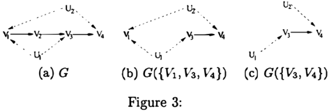
Consider Figure 3(a), which has two c-components {V2} and S = {V1, V3, v.}. The only admissible or­ der is V, < V2 < V3 < v ·. Applying Corollary 1, we obtain

In the subgraph G(S) = Gsuu (Figure 3(b)), v, is not an ancestor of H = {Vj, v.}, and from Lemma 1, summing both sides of (33) over V,, we obtain

The subgraph G(H) = GHuu (Figure 3(c)) has two c-components {V3} and {V.}. By Lemma 2, we have Q[H] = Q[{V3}]Q[{V4}], and

Eq. (36) implies a constraint on P( v ) that the right hand side is independent of v2.

From the preceding examples, we see that we may find constraints by alternatively applying Lemma 1 and 2. Next, we present a procedure that systematically look­ ing for constraints.

4.2 Identifying constraints systematically

Let a topological order over V be V1 < ... < Vn, and let V(i) = {V1, ... ,V;}, i = 1, ... ,n. Fori from 1 to n, at each step, we will look for constraints that involve V; and the variables ordered before V;. At step i, we do the following:

• (A1) Consider the subgraph G(V(i)). If G(V(i)) has more than one c-component, assuming that V; is in the c-component S; of G(V(i)), then by Corol­ lary 1, Q[S;] is computable from P(v) and may give a conditional independence constraint that V; is independent of its predecessors given its ef­ fective parents, other variables in S;, and the effective parents of other variables in S;, that is, V; is independent of V(i) \ Pa+(S;) given Pa+(S;) \ {V;}.
• (A2) Consider Q[S;] in the subgraph G(S;). For each descendent set D C S; (D contains its own ob­ served descendants) in G(S;) that does not con­ tain V;, 4 by Lemma 1 we have

The left hand side of (37) is a function of Pa+(S;) \ D, while the right hand side is a func­ tion of Pa+(s; \D)� Pa+(S;) \D. Therefore, if some effective parents of D are not effective par­ ents of S; \ D, then (37) implies a constraint on the distribution P(v) that the quantity Ld Q[S;] is independent of (Pa+(S;) \D)\ Pa+(S; \D).

Let D' = S; \ D. Next we consider Q[D'] in the subgraph G(D'). If G(D') has more than one c-component, assuming that V; is in the c­ component E; of G(D'), by Lemma 2, Q[E;] is computable from Q[D'], and Q[D']/ Lv; Q[D'] is a function only of Pa+(E;), which imposes a con­ straint on P(v) if Pa+(D') \ Pa+(E;) =f 0.

Finally we study Q[E;] by repeating the process (A2) with S; now replaced by E;.

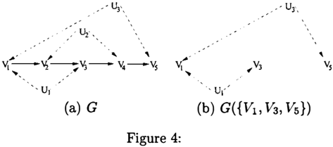
The preceding analysis gives us a recursive procedure for systematically finding constraints. To illustrate this process, we consider the example in Figure 4( a). The only admissible order over V is Vi < .. . < Vs. The constraints involving V, to V4 are the same as in Figure 2, and here we look for constraints involving Vi;. Vs is in the c-component S = {V,, Vj, Vs}. By

4We need to consider every descendent set D that does not contain v;, because it is possible that for two descen­ dent sets D1 C D 2 , the constraints from summing D 2 are not implied by that from D,, and vice versa.

Corollary 1, Q[SJ is given by

which implies no constraints. In the subgraph G(S) (Figure 4(b)), the descendent sets not containing Vs are {Vi}, {V3}, and {V1, V3}.

(a) Summing both sides of (38) over v1, we obtain

which implies no constraints. The subgraph G({V3, Vs}) is partitioned into two c-components {V3} and {Vs}, and by Lemma 2, we have

which implies a constraint that the right hand side is independent of v2 and V3.

(b) Summing both sides of (38) over V3, we obtain

which implies a constraint that the right hand side is independent of V2. G ( { vl' Vs}) can not be further partitioned into c-components.

(c) Summing both sides of (38) over v1 and va, we obtain

which implies a constraint that the right hand side is independent of v2. This constraint is implied by that obtained from Eq. (40).

5 Projection to Semi-Markovian Models

If, in a Bayesian network with hidden variables, each hidden variable is a root node with exactly two ob­ served children, then the corresponding model is called a semi-Markovian model. The examples we have stud­ ied in Figure 1, 3, and 4 are semi-Markovian models while Figure 2 is not. Semi-Markovian models are easy to work with, and we will show that a Bayesian net­ work with arbitrary hidden variables can be converted to a semi-Markovian model with exactly the same set of constraints (that can be found through the proce­ dure in Section 4.2) on the observed distribution P(v).

5.1 Semi-Markovian models

In a semi-Markovian model, the observed distribution P( v) in (3) becomes

And the quantity Q[SJ in (5) becomes

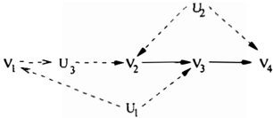
It is convenient to represent a semi-Markovian model with a graph G that does not show the elements of U explicitly but, instead, represents divergent edges Vi +u k --+ Vj with a bidirected edge between Vi and Vj. For example, Figure 3(a) will be represented by Figure 5. It is easy to partition such a graph into c-components. Let a path composed entirely of bidi­ rected edges be called a bidirected path. Two observed variables are in the same c-component if and only if they are connected by a bidirected path. Letting Pa(S) denote the union of S and the set of parents of S, then it is clear that Q[S] is a function of Pa(S). In Lemma 1 and 2, G(C) (G(H)) will be replaced by Gc (GH), and Pa+(-) replaced by Pa(·).

5.2 Projection

A Bayesian network with arbitrary hidden variables can be converted to a semi-Markovian model by con-

structing its projection [Verma, 1993].

Definition 1 (Projection) The projection of a DAG G over V U U on the set V, denoted by PJ(G, V), is a DAG over V with bidirected edges constructed as follows:

1. Add each variable in V as a node of PJ(G, V).
2. For each pair of variables X, Y E V, if there is an edge between them in G, add the edge to PJ(G, V).
3. For each pair of variables X, Y E V, if there exists a directed path from X to Y in G such that every internal node on the path is in U, add edge X --+ Y to PJ(G, V) (if it does not exist yet).
4. For each pair of variables X, Y E V, if there exists a divergent path between X and Y in G such that every internal node on the path is in U (X +­ U; --+ Y ) , add a bidirected edge X +---+ Y to PJ(G, V).

It is shown in [Verma, 1993] that G and PJ(G, V) have the same set of conditional independence rela­ tions among V . Next we show that the procedure presented in Section 4.2 will find the same sets of con­ straints on P(v) in G and P J(G, V). To this pur­ pose, we need to show that for any set H <;;; V, G and PJ(G, V) have the same arguments for Q[H], the same topological relations over H, and the same sets of c-components.

Lemma 3 For any set H <;;; V, Q[H] has the same arguments in G and PJ(G, V), that is, Pa + (H) in G is equal to Pa(H) in PJ(G, V).

Lemma 3 is obvious from Definition 1.

Lemma 4 For any setH <;;; V , and any two variables V;, Vj E H, Vi is an ancestor ofVj in G(H) if and only if V; is an ancestor ofVj in PJ(G, V)H (the subgraph of PJ(G, V) composed only of variables in H).

Lemma 4 has been shown in [Verma, 1993].

Lemma 5 For any set H <;;; V, G(H) is partitioned into the same set of c-components as PJ(G, V)H·

The proof of Lemma 5 is given in the Appendix.

By Lemma 3-5, we conclude that the procedure pre­ sented in Section 4.2 will find the same sets of con­ straints on P(v) in G and PJ(G, V). Since it is eas­ ier to work in a semi-Markovian model, we can always convert a Bayesian network with arbitrary hidden vari­ ables to a semi-Markovian model before searching for constraints on the distribution P(v).

6 Conclusion

This paper develops a systematic procedure of identi­ fying functional constraints induced by Bayesian net­ works with hidden variables. The procedure can be used for devising tests for validating causal models, and for inferring the structures of such models from observed data. At this stage of research we cannot as­ certain whether all functional constraints can be iden­ tified by our procedure; however, we could not rule out this possibility.

Acknowledgements

This research was supported in parts by grants from NSF, ONR, AFOSR, and DoD MURI program.

References

• [Desjardins, 1999] B. Desjardins. On the theoretical limits to reliable causal inference. PhD thesis, U ni­ versity of Pittsburgh, 1999.

[Geiger and Meek, 1998] Dan Geiger and Christopher Meek. Graphical models and exponential families. In Proceedings of the Fourteenth Annual Conference on Uncertainty in Artificial Intelligence (UAI- g s), pages 156-165, San Francisco, CA, 1998. Morgan Kaufmann Publishers.

[Geiger and Meek, 1999] Dan Geiger and Christopher Meek. Quantifier elimination for statistical prob­ lems. In Proceedings of the Fifteenth Annual Confer­ ence on Uncertainty in Artificial Intelligence (UAI99), pages 226-235, San Francisco, CA, 1999. Mor­ gan Kaufmann Publishers.

[Pearl et al., 1990] J. Pearl, D. Geiger, and T. Verma. The logic of influence diagrams. In R.M. Oliver and J.Q. Smith, editors, Influence Diagrams, Belief Nets and Decision Analysis, pages 67-87. John Wiley and Sons, Inc., New York, NY, 1990.

[Pearl, 1988] J. Pearl. Probabilistic Reasoning in In­ telligence Systems. Morgan Kaufmann, San Mateo, CA, 1988.

[Pearl, 1995] J. Pearl. On the testability of causal models with latent and instrumental variables. In P. Besnard and S. Hanks, editors, Uncertainty in Artificial Intelligence 11, pages 435-443. Morgan Kaufmann, 1995.

[Robins and Wasserman, 1997] James M. Robins and Larry A. Wasserman. Estimation of effects of se­ quential treatments by reparameterizing directed

--!

acyclic graphs. In Proceedings of the Thirteenth An­ nual Conference on Uncertainty in Artificial Intelli­ gence (UAI-97}, pages 409-420, San Francisco, CA, 1997. Morgan Kaufmann Publishers.

[Spirtes et a/., 1993] P. Spirtes, C. Glymour, and R. Scheines. Causation, Prediction, and Search. Springer-Verlag, New York, 1993.

[Tian and Pearl, 2002] J. Tian and J. Pearl. A gen­ eral identification condition for causal effects. To appear in Proceedings of the National Conference on Artificial Intelligence (AAAI) 2002.

[Verma and Pearl, 1990] T. Verma and J. Pearl. Equivalence and synthesis of causal models. In P. Bonissone et al., editor, Uncertainty in Artifi­ cial Intelligence 6, pages 220-227. Elsevier Science, Cambridge, MA, 1990.

[Verma, 1993] T. S. Verma. Graphical aspects of causal models. Technical Report R-191, Computer Science Department, University of California, Los Angles, 1993.

Appendix: Proof of Lemma 5

Lemma 5 For any set H <; V, G(H) is partitioned into the same set of c-components asP J(G, V)H.

Proof: (1) If two variables X, Y E H are in the same c-component in PJ(G, V)H, then there is a bidirected path between X andY in PJ(G, V)H:

From the definition of a projection, there is a path between X and Y in G(H) on which each observable is head-to-head:

Therefore X and Y are in the same c-component in G(H).

(2) If X, Y E Hare in the same c-component in G(H), then there exist Ui and Ui such that Ui is a parent of X, Ui is a parent of Y , and Ui = Ui or there is a path p between Ui and Ui such that every observable on p is head-to-head and every hidden variable on p is in U(H). We prove that X and Y are in the same c­ component in PJ(G, V)H by induction on the number k of head-to-head nodes on p.

Base: k = 0. There is no head-to-head node on p, then there is a divergent path between X and Y in G:

Therefore there is a bidirected edge X +---+ Y in PJ(G, V)H, and X and Y are in the same c­ component in PJ(G, V)H·

Induction hypothesis: If there are k head-to-head nodes on p, X and Y are in the same c-component in PJ(G, V)H·

If there are k + 1 head-to-head nodes on p, let W be the head-to-head node closest to X on p. If W is an observable, let V; = W, otherwise let V; be an observable descendant of W such that there is a directed path from W to V; on which all internal nodes are hidden variables. From the base case, X and V; are in the same c-component in PJ(G, V)H, and from the induction hypothesis, V; and Y are in the same c-component in PJ(G, V)H, hence we have that X and Y are in the same c-component in PJ(G, V)H. o