Optimal Limited Contingency Planning

Nicolas Meuleau* and David E. Smith

NASA Ames Research Center Mail Stop 269-3

Moffet Field, CA 94035-1000 { nmeuleau, de2smith} @email.arc.nasa.gov

Abstract

For a given problem, the optimal Markov policy over a finite horizon is a conditional plan contain­ ing a potentially large number of branches. How­ ever, there are applications where it is desirable to strictly limit the number of decision points and branches in a plan. This raises the question of how one goes about finding optimal plans con­ taining only a limited number of branches. In this paper, we present an any-time algorithm for optimal k-contingency planning. It is the first op­ timal algorithm for limited contingency planning that is not an explicit enumeration of possible contingent plans. By modelling the problem as a partially observable Markov decision process, it implements the Bellman optimality principle and prunes the solution space. We present ex­ perimental results of applying this algorithm to some simple test cases.

1 INTRODUCTION

Markov decision processes (MDPs) provide a powerful the­ oretical framework for planning under uncertainty with probabilities, costs and rewards [15]. In this framework, the optimal solution to a problem is an optimal policy, that is, a rule specifying the action to perform for each situa­ tion we could possibly be in. For a finite planning horizon, this policy represents a conditional or contingent plan with a branch for each possible situation that might be encoun­ tered during execution. Therefore, the optimal contingent plan may be large and complex, since it may contain a large number of branches.

There are applications where this size and complexity is a significant drawback. Consider, for example, the problem of constructing daily plans for a Mars rover. There is a great deal of uncertainty in this domain, concerning such things

· QSS Group Inc.

as time, energy usage, data storage available, and position (see [5] for a more detailed description). However, there are some compelling reasons for keeping the plans simple:

• There is a need for cognitive simplicity - plans must be simple enough that they can be displayed easily, and understood and modified by both Earth scientists and mission operations personnel.
• Plans must undergo very detailed analysis and simu­ lation using complex models of illumination, energy consumption, thermal characteristics, kinematics, and terrain. There is limited time to do this analysis, so plans must be kept structurally simple in order to ex­ pedite this process.
• There is limited communication bandwidth and lim­ ited storage on board the rover, so there is an advan­ tage to keeping plans small.

As a result, we are interested in limited contingency plan­ ning. More precisely, we would like to be able to compute the optimal k-contingency plan for a problem- that is, the optimal plan containing k or fewer contingency branches.

In general, the problem of contingency planning is known to be quite hard [ 11], and k-contingency planning is no exception. If k = oo, k-contingency planning reduces to finding the optimal policy. If k = 0, k-contingency plan­ ning reduces to stochastic conformant planning, where we must find the best unconditional sequence of actions [9]. One can argue that limited contingency planning is harder than both conformant planning and searching for the opti­ mal policy. First, the search space of conformant planing (that is, the set of all sequences of actions) is exponentially smaller than the search space of k-contingency planning (the set of all k-contingency plans). Second, although the set of all policies is usually larger than the set of all k­ contingency plans, dynamic programming (DP) techniques are able to significantly prune the search for an optimal policy by using Bellman's optimality principle. However, to our knowledge, there is no previous algorithm that is

able to implement Bellman's optimality principle for lim­ ited contingency planning. The problem is that the classi­ cal Markov state is insufficient: knowing the best limited contingency plan from time t + 1 to the horizon for each state we could be in at time t + 1 does not help to find the best plan from time t to the horizon . In fact, the action performed at time t may bring us no certainty about the state at time t + 1, and the best plan for an uncertain ini­ tial state may be different from the best plan in each state. However, the belief-state borrowed from partially observ­ able Markov decision process (POMDP) theory [6, 10] , that is, a probability distribution on the original state, is a suf­ ficient statistic to allow a DP approach to the problem of limited contingency planning. This is the basic principle of the algorithm presented in this paper.

Conformant planning is well known to be equivalent to the problem of planning in an unobservable environment: lim­ iting oneself to unconditional plans is equivalent to dis­ carding the observation of the current state that is avail­ able at each time step. The first algorithm to exploit this fact performed heuristic search through the belief space [1, 4]. Instead of using Bellman's optimality principle, these techniques (when they tackle the optimal planning problem) rely on admissible heuristics to prune the search space [4]. Recently, Hyafil and Bacchus used the best so­ lution techniques for POMDPs to solve stochastic confor­ mant planning problems [9]. In this approach, conformant planning is modelled as a fully non-observable Markov de­ cision process (NOMDP), which is a particular case of a POMDP. As Hyafil and Bacchus point out, the drawback of this approach is that it requires computing optimal so­ lutions for states that may be unreachable, but its strength is that it prunes the search space by using Bellman's op­ timality principle . For several test bed problems, Hyafil and Bacchus show that this approach outperforms a CSP algorithm that is able to do some reachability analysis but cannot prune the search space. Moreover, the superiority of the POMDP approach becomes apparent as the size of the problems grows.

In this paper, we present optimal k-contingency planning (OKP), an incremental algorithm for optimal limited con­ tingency planning. As in [9], we use a POMDP framework to model the problem, which allows using Bellman's op­ timality principle to speed up the search. The difference is that we must encode the number of branches allowed in the state description of the POMDP . In effect, this amounts to keeping multiple copies of the POMDP corresponding to different numbers of branches allowed. When we choose to make an observation in one POMDP, we drop into a POMDP with fewer branches allowed. When all the branches are used up, we end up in the POMDP for the conformant plan­ ning problem as used by Hyafil and Bacchus .

We start by specifying the notion of contingent plan used throughout the paper. In Section 2, we first show how

Hyafil and Bacchus encoded conformant planning as a POMDP. We then move on to !-contingency planning, fol­ lowed by balanced k-contingency planning. In Section 3 we further generalize this to arbitrary k-contingency plan­ ning. In Section 4 we present experimental results compar­ ing OKP against a brute force search technique for finding k-contingency plans. Finally, we review related work and conclude.

1.1 CONTINGENT PLANS

This paper addresses a series of variants of the limited con­ tingency planning problem. In general, we are looking for optimal tree-shaped plans, the simplest form being confor­ mant plans, which are simple sequences of actions without branches. This choice may seem a little odd since there are more compact types of plans or policies, such as finite state controllers. However, there are reasons to prefer tree­ shaped plans in some application domains. For instance, in the Mars rover domain, resources are monotonically de­ creasing along each possible trajectory, so that a state is never visited twice. Moreover, the action the rover executes must depend on the resource available. Therefore, NASA requires that plans have finite horizon and do not contain loops.

Optimal k-contingency planning is the problem of finding an optimal tree-shaped plan with (at most) k branch points. We consider three variants of this problem:

general k-contingency planning: in the most general case, we are looking for the best plan with at most k branch points overall;

linear k-contingency planning: we try to find the best plan with at most k branch points, all of them on one trajectory through the plan. That is, the plan structure is a main line of actions with simple branches attached to it, and no branches on the branches.

balanced k-contingency planning: we are looking for the best plan with at most k branch points in each pos­ sible trajectory through the plan. That is, the largest possible plan structure is a balanced tree with k branch points in each path from the root (initial time) to a leaf (planning horizon). So, there are actually more than k branch points over the whole plan.

Although the balanced plan structure is a bit contrived, it is useful for presenting our algorithm since OKP takes its simplest form in this case.

2 OPTIMAL BALANCED k-CONTINGENCY PLANNING

Our formalism uses several POMDPS defined over different state, action and observation spaces, so it is important to

understand the role of each POMDP. The first POMDP we introduce, M, represents the planning problem in the clas­ sical sense. In this paper, our goal is to find optimal contin­ gent plans for the process M. M can be a fully observable MDP, which we see as a particular case of a POMDP. In our framework, it means that we can observe exactly the current state each time we decide to branch. In the general case (when M is not an MDP), we have only noisy observa­ tions for branching decisions. Later, we introduce several other POMDPs, {Mk : k :;:: 0}, obtained by transforming the original process M in such a way that an optimal so­ lution to Mk is an optimal k-contingency plan for M. So, each Mk represents the problem ofk-contingency planning inM.

The planning problem for which we want to find opti­ mal contingent plans is modelled as the POMDP lvf = (S,A,n,T,R,O), where S, A and n are the (finite) set of states, actions and observations (respectively); T is the transition probability: T ( s, a, s') is the probability of mov­ ing to state s' if we execute action a in state s; R is the reward function: R(s, a) is the (expected) reward for exe­ cuting action a in state s; and 0 is the observation prob­ ability: 0( a, s', o) is the probability of observing o E n when an execution of action a leads to state s'. In this sec­ tion, we assume that the observation probabilities of M do not depend on the last action executed, and we denote by O(s', o ) the (well defined) probability of observing o E n when arriving in s ' E S. We relax this assumption in Sec­ tion 3.3. If M is a fully-observable MDP, then n = S and O(s', s ') = 1 for a i l s' E S.

The problem we tackle is this section is the following: given M, H, and a probability distribution over the initial state x 0 ( s ) (the initial belief), find the best contingent plan where there are (at most) k branch points in each possible trajectory through the plan. The optimality criterion used is the classical expected cumulative reward (discounted or not) up to the planning horizon H:

r(t) is the reward received at timet and-y E [0, 1] is the discount factor.

First, we assume that we must create one branch for each observation that can be made at each branch point (so, the branch points are 101-ary in a POMDP, and ISI-ary in an MDP). We show how to relax this constraint in Section 3.2.

2.1 CONFORMANT PLANNING

When k = 0, the problem is that of conformant planning: we must find the best unconditional sequence of H ac­ tions. As Hyafil and Bacchus [9] , we model the stochas­ tic conformant planning problem as a completely non ob­ servable MDP (NOMDP) M 0 = (S0 A0 no T0 R0 oo) ' ' ' ' '

where S0 = S; A0 = A; no contains only one ele­ ment, o0, that basically says "/ can't see anything infor­ mative"; T0(s, a, s') = T(s, a, s'), R0(s, a) = R(s, a), and 0°(a, 8 1 , o0) = 1 for all (s, a, s') E s X A X s.

As for any POMDP [10], the optimal solution of M0 over the finite horizon H can be determined in finite time using value iteration (VI), which is a form of dynamic program­ ming (DP). Starting from the planning horizon H, we pro­ ceed backward through time to construct a value function V1° for each t E {0; 1; .. . H}. The value V';0(x) represents the expected reward we get by executing an optimal confor­ mant plan for the starting belief x over the planning horizon t. In the particular case of the NOMDP M 0 , the equations of VI are the following (the superscript 0 of the V and Q functions is a reference to k, the number of branch points iu the plan):

and, for all t E {0, 1, ... H- 1}:

8� 0 (x) represents the belief posterior to action a and ob­ servation o0, given the prior belief x. It is given by Bayes' rule:

Since we do not make any observation at all, whether the original process M is a POMDP or an MDP does not influ­ ence in any way the optimal solution of conformant plan­ ning. Note that the observation set n and the observation function 0 are not used anywhere in the equations above.

Practical implementations of VI exploit the fact that the value function is always a piecewise linear convex func­ tion of the belief x. The functions Y';0(-) and Q�(·, a) are represented as finite sets of a-vectors, each of them corre­ sponding to a linear function of x. V';0 and Q� are then de­ fined as the supremum (max) of the set of linear functions that represent them. All operations in equations (2) and (3) reduce to manipulation and production of a-vectors. The sets of a-vectors are regularly purged of vectors represent­ ing linear functions that are optimal nowhere in the belief space. Many algorithms differ only in the way they purge sets of a-vectors. Although the belief space is continuous, all the computation is finite [10, 6].

The value function constructed when solving M0 up to the planning horizon H contains the expected reward of the best conformant plan in each possible initial belief state, and for each planning horizon less than or equal to H. To get the optimal plan for a particular starting belief x 0 (for instance, the certainty of being in a given state) and horizon

H, we must simulate a trajectory by always executing the optimal action for the current belief state, which requires monitoring the belief state along the trajectory using equa­ tion ( 4 ) . Since there is only one possible observation at each step, there is always only one possible belief at the next step. So, the trajectory can never branch.1 We could as easily extract the optimal conformant plan for another starting belief and/or another planning horizon h < H. All the information that is important and hard to calculate is in the value function, which is computed only once. In OKP, we do not need to extract any plan before having reached the level k where we decide to stop.

2.2 I-CONTINGENCY PLANNING

Similarly, the optimal !-contingency plan is the optimal so­ lution of a POMDP M 1 = (51 A 1 !)\ T1 R1 01) M 1 is ' ' ' ' ' . constructed by duplicating M0 and adding an observe-andbranch action between the two copies of M0· Thus, each state s E S of the original POMDP M is represented twice in M1. One copy represents being in s before the plan has branched, and the other represents being in s after the plan has branched. The observe-and-branch action induces an irreversible transition from states of the first type to states of the second type. As fork = 0, the problem is completely non-observable, except that the observe-and-branch action allows making an ordinary observation as specified in the original POMDP M, and conditioning the next actions on this observation. If M is an MDP, then the observe-and­ branch action sees the current state exactly. Formally:

States: 51 = S x {0, 1}. The pair (s,k), s E S and k E { 0, 1} , represents being in s and having possibility of using the observe-and-branch action k times in the future. Each ( s, 0) may be seen as an element of S0, the state space of the conformant planning NOMDP M0.

Belief states: The number of branch points that are still available for the future, k, is always known with certainty. All the uncertainty on the state ( s, k) of M1 comes from the uncertainty on s. Therefore, a belief state for M1 is a pair (x, k) where xis a probability distribution overS and k E {0,1}.

Actions: A1 =AU {a0b}, where aob is the observe-and­ branch action. aob is executable only in states (s, 1), s E S. a0b is a special instantaneous action: executing it does not increment time. As shown below, it can be used only

1 !t is also possible to simulate trajectories by following point­ ers from a-vectors at timet to a-vectors at timet+ 1 established when solving M0, instead of maintaining the current belief. How­ ever, this technique appeared to be much slower in the context of OKP with k > 0, because it does not allow not building a branch for observations that are impossible given the current belief dur­ ing plan extraction.

once in each trajectory. The other actions a E A are called ordinary actions.

Observations: Formally, !V = !1. However, useful observations can be made only through the observe-and­ branch action a0b. All other actions provide a non informa­ tive observation. To model this, we select arbitrarily one observation of the original process, we rename it o 0 , and we use it to represent the non-informative observation pro­ duced by all actions different from a0b. Observed after an ordinary action a E A, a0 means "/ can't see anything in­ teresting", and when it is observed after a0b, it has the same semantics as in the original process M.

Effects of ordinary actions: The states (s, 0), s E S, represent an absorbing subset, that is, we cannot get out of this subset once we enter it (remember that only or­ dinary actions are possible in such states). All the tran­ sition probabilities, rewards and observation probabilities involving only such states are defined as in M0. The only way to get out from states of type (s, 1), s E S, is through the observe-and-branch action. The transi­ tion probabilities, reward and observations involving only states of the type ( s, 1), s E S, and not the observe­ and-branch action a0b, are also defined exactly as the transitions, rewards, and observations in M0. That is: T1((s,k),a, (s',k)) = T(s,a,s'), R1((s,k),a,(s',k)) = R(s,a,s'),and01(a,(s',k),o0) = 1 ,for all ( s ,k,a,s') E s X {0; 1} X A X s.

Effect of the observe-and-branch action: executing ac­ tion a0b in state (s, 1) leads with certainty to state (s, 0), with the same number of time-steps to go. This action pro­ vides no reward and produces an observation following the observation probability of the original POMDP. Formally: T1((s, 1), a0b, (s, 0)) = 1, R1 ((s, 1), aob, (s, 0)) = 0, and 01(a0b, (s,O),o) = O(s,o), for all (s,o) E S x !1.

The fact that the observe-and-branch action is instanta­ neous might make the solution of M1 with VI look a little bit complicated a priori. However, it turns out that opti­ mization over a finite horizon is straightforward. First, for all x and all t :::; H, the value of belief state ( x, 0) at time t in M1 is equal to yt0(x) in M0. In other words, the result of the computation at level 0 (equations (1) through (3)) can be reused as is, it gives the value of each belief state (x,O) ofM1 at allt E {0,1, ... H}. Then,if we denote by yt1(x) the value at timet of belief (x, 1) in M1, then VI is summarized by the following equations:

and, for all t E {0, 1, ... H1}:

with

for all a E A (using equation ( 4) to calculate 8�0 ( x) ), and

where B�·' (x) is the posterior belief after observing o, given by Bayes'rule:

Note that if the original problem is an MDP, then equations (8) through (9) simplify as:

where belief x 8 gives state s with probability I.

So, a practical solution of M1 requires (i) having solved M0 in advance; and (ii) one (backward) pass of VI through states ( s, 1), s E S, following equations (5) to (11). During the calculation of V1, we read a-vectors in the solution of M0 to evaluate the observe-and-branch actions. Once tbe value function V1 is calculated, we can extract the optimal !-contingency plan for a given initial belief x 0 by simulat­ ing a trajectory in M1. As long as the observe-and-branch action is not used, the trajectory may never branch. If at some point the Q -values Ql indicate that a0b is the opti­ mal action for the current belief state, tben a branch point is added to the plan. We must then calculate the poste­ rior belief for each observation o E !1 using equation (I 0) (that is, for each state s E S if M is an MDP). Finally, the optimal branch for each o is constructed by simulat­ ing a (non-branching) trajectory in M0· Because a0b is not present in M0, no more branch points can be added. Note that it may happen that the observe-and-branch action is never used during the travel through M1. It shows tbat there exists a conformant plan that is at least as good as the best ! -contingency plan, so there is no need to use an observe-and branch action. Note also that, one more time, the optimal solution of M1 contains the value of the best k-contingency plan for all k E {0, 1 }, all possible initial beliefs xo, and all planning horizons less than or equal to H.

2.3 BALANCED k-CONTINGENCY PLANNING

In general, the k-contingency planning problem (k � 2) may be modelled as a POMDP Mk built on Mk-l by adding a copy of 5° connected to the (k - 1)t h level of Mk-l by the observe-and-branch action. All the equations of tbe previous section can be re-used by replacing superscript I by k and superscript 0 by k -1. That is:

If the solution of Mk-l is known, then the solution of Mk requires only one pass of VI through states at level k (that is, states (s, k), s E 5), reading a-vectors in v;k-l to eval­ uate the observe-and-branch action. Once the value func­ tions v;k are determined, we can easily extract the best (bal­ anced) k-contingency plan for a given initial belief by sim­ ulating a trajectory in Mk. When the observe-and-branch action is used, the trajectory branches and one branch for each possible observation o E !1 must be built by simulat­ ing a trajectory in Mk-l. This is why tbe algorithm pro­ duces balanced contingency plans: at each branch point at level l � k, each exiting branch (which is in fact a tree) may contain up to l-1 branch points (equation (16)). Therefore, each trajectory through tbe plan tree may tra­ verse up to k branch points. As previously, tbe algorithm does not have to use all the branch points allowed if there is no utility to be gained by doing so. Therefore, the version of OKP presented in tbis section produces an optimal plan with at most k branch points in each trajectory. 2

3 EXTENSIONS

OKP may easily be adapted to other variants of the limited contingency planning problem.

3.1 TYPES OF PLANS

First, the algorithm can search for other types of plans. For instance, we can search for the optimal linear k­ contingency plan as defined in Section 1.1, that is, tbe best plan with (at most) k branch points, all of them on

2 Note that the plan extraction phase of this version of OKP is exponential in k. This is an artifact due to the particular variant of the problem addressed. What we call a "balanced k-contingency" plan contains in fact a number of branch points exponential in k. Therefore, extracting such a plan from the solution of the POMDP is exponential in k. This is not the case for the other variants of the algorithm presented in Section 3.1.

one trajectory through the plan. In this case, each level l E {1, 2, ... k} of Mk contains 1!11 observe-and-branch actions, {a�b,o E !1}. The semantics of a�b is "observe, branch, and use the l -1 remaining branch points in the branch associated with observation o". Equation (13) be­ comes

where

Similarly, we can tackle the general k-contingency plan­ ning problem (at most k branches over the whole plan with­ out any other constraint), by adding multiple observe-and­ branch actions at each level of Mk. Here we must model one observe-and-branch action for each possible way to distribute the k - 1 remaining branch points in the 1!11 ex­ iting branches. Therefore, the number of different observe­ and-branch actions required at level k is

So this variant of OKP is somewhat impractical for large k. As shown below, a way to limit the complexity of the algorithm is to change the branch conditions.

3.2 BRANCH CONDITIONS

The algorithm of Section 2 creates one particular branch for each observation o E !1 that can possibly be made after the observe-and-branch action (although it considers only the observations that are possible given the current belief during plan extraction). In other words, there may be up to 1!11 branches stemming from each branch point of the plan. In some variants of the limited contingency planning prob­ lem, we may want to limit the number of branches exiting from each branch point by grouping several observations together.

OKP can be adapted to any kind of branch condition. For instance, if we want the plan to use binary branch points, then we must create one observe-and-branch action a0� for each possible way to partition the observation set !1 into two non-empty subsets !1' and !1 \ !1 ' . Equation (13) be­ comes

where

and similarly for Q;(x, a0�, !1 \ !1'). Note that there are 21°1 - 2 such actions (subsets !1'), which is a considerable number in most cases.

The equations above correspond to balanced k-contingency planning. If we are looking for other types of plans, then we must create a different observe-and-branch action for each possible branch condition and each possible way of distributing the remaining branch points in the stemming branches. However, the number of ways of distributing branch points is greatly reduced (compared to the formulas of Section 3.1) when we use compact branch conditions. For instance, if we look for the optimal plan with at most k binary branch points overall, then there are 21°1 - 2 dif­ ferent branch conditions, but only k ways to distribute the k 1 remaining branch points in the two exiting branches. Therefore, the total number of observe-and-branch actions at level k is (21°1 -2)k.

The computational price of compact branch conditions can be greatly reduced in the particular case where the obser­ vation o represents a numerical value.3 In this case, we can focus the search on a particular kind of branch condi­ tion based on threshold. Each branch point is defined by a threshold aT E 0. There are two exiting branches: one corresponds to observing a value o E 0 less than or equal to or, and the other corresponds to values greater than aT. Thus, the total number of different branch conditions is 1!11 - 1. As there are only two exiting branches, there are only k ways to distribute the remaining branch points. Therefore, the total number of observe-and-branch actions at level k of the strict k-contingency planning POMDP is only (1!11- 1)k.

3.3 GENERAL POMDPS

Finally we can relax the hypothesis on the observation probabilities of the original POMDP M. In Section 2, we as­ sumed that the observation probabilities depend only on the arrival state s ' (that is, O(s', o)), while the general formal­ ism of POMDPs assumes that they also depend on the last action ( 0( a, s', o) ), which allows a richer model of sensory actions. The problem is that, when we move to this more general framework, the observation probabilities of a0b in Mk,previously defined as0k(a0b,(s,k-1),o) = O(s,o), are not well defined anymore. The observation following the use of the observe-and-branch action depends on the action performed at the previous time step, which violates the (first order) Markov property.

3 Actually, it is not necessary that the observation is a numericalvariable.It is sufficient that therebe a complete order defined over it.

One way to deal with this situation is to introduce the last action executed into the Markov state of M k . Another, equivalent, way to model this is as follows: instead of adding Nk observe-and-branch actions to the preexisting JAJ actions at each level k (where Nk is the total number of branch conditions and ways of distributing k -1 remain­ ing branch points in the exiting branches), we create Nk (new) copies of each action a E A. Each copy corresponds to executing a, and then branching the plan following the protocol of a particular observe-and-branch action. For in­ stance, in the case of balanced k-contingency planning with J ! 1J-ary branch points (as in Secti�n 2), we duplicate each action a E A and call a its copy (A is the set of all copies). a represents executing a, not discarding the resulting ob­ servation, and branching the plan based on this observation following the protocol of action a0b of Section 2. The equa­ tions of vr become:

Note that we are not concerned with this issue if the original process M is a fully observable MDP.

4 EXPERIMENTS

We implemented OKP using Cassandra's POMDP solver available on the Internet.4 We used the witness algorithm [10] to solve OKP's multiple level POMDP. The results presented in this paper concern the variant of OKP that searches for balanced contingent plans (Section 3.1 ), build­ ing a branch for each possible observation (Section 3.2). We focus on two simple test bed problems.

As Hyafil and Bacchus stressed for the particular case k = 0, OKP for general k is able to prune the plan space (using Bellman's optimality principle), but it computes (the value of) the optimal plan in every belief state at every hori­ zon, while we may be interested only in a single initial be­ lief and the belief states reachable from it. To measure the value of this trade-off, we implemented in the same envi­ ronment as OKP, an algorithm that systematically searches and evaluates all possible contingent plans for a given k, horizon, and initial belief, taking into account only reach­ able belief states. Its performance gives an indication of the

4http://www.cs.brown.edu/research/ai/pomdp/

size of the search space, and how OKP is able to prune the search using Bellman's optimality principle.

The first problem we used is a variant of the tiger problem [10]. In this problem, the agent is standing in front of two doors (left and right). Behind one door lies a dangerous tiger, and there is a reward behind the other door. There­ fore, there are two different world states: tiger-left and tiger-right. The initial position of the tiger is unknown, and the initial probability on the tiger position is uniform over the two doors. The agent has three possible actions: opening one of the doors (open-left and open-right), or lis­ tening to try to guess where the tiger is (listen). The listen action does not change the state of the world, it costs I unit of utility, and provides a noisy observation that can take two possible values: hear-tiger-left and hear-tiger-right. If the state of the world is tiger-leji, then the probability of observing hear-tiger-left is 0.85 and the probability of ob­ serving hear-tiger-right is 0.15. Similarly, the probability of hearing the tiger to the right when the tiger is actually to the right is 0.85. Opening the door behind which the tiger lies provides a "reward" of -10. Opening the other door brings a reward of +6. After opening a door, the problem is reset in its original state (that is, the agent is brought back in front of the doors and the new position of the tiger is drawn at random uniformly). Given these parameters, the optimal conformant plan over a horizon of H time-steps is to listen H times. At each step, it provides the reward -1 with cer­ tainty, while opening an arbitrary door (we are not allowed to condition the choice of the door on the result of previous listen actions) brings the expected reward: 0.5 (-10) + 0.5 (6) = -2. The discount factor is set to I (no discount).

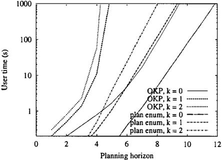
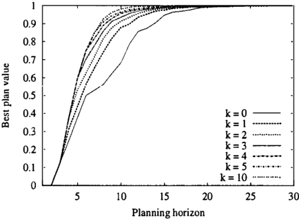
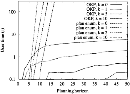
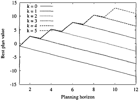
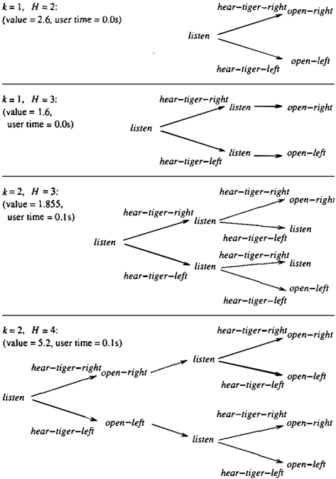
We ran OKP and plan enumeration on the tiger problem for different planning horizons H and levels k. Fig. I shows the optimal contingent plans obtained with a sam­ ple of small values for H and k. Fig. 2 shows the evolution of the value of the optimal contingent plan as a function of k and H. Finally, Fig. 3 shows the evolution of the to­ tal time taken by the algorithm as a function of k and H. These results clearly show the exponential blow-up of the search space and how o KP is able to resist it by efficiently pruning the search. In this example, Bellman's optimality principle allows a drastic reduction in the complexity of the search that largely compensates for the fact that we have to deal with (belief) states that are unreachable.

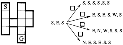
The second problem is a small maze world due to Horstmann and Zilberstein [8] and represented in Fig. 4. In this problem, the agent starts from the location marked with an S and must end-up in the goal location G. The agent can use 4 actions, N, S, E and W, that allow it to move 1 or 2 positions in the desired direction with equal probability (unless a wall blocks the way). The goal state is absorbing. The observation available (when we decide to branch) is the presence or absence of a wall on each side of the square that defines the agent's location. Thus, there are 8 different

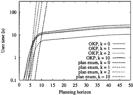
possible observations (and 11 states). The agent gets a zero reward at every step except when it enters the goal state. Therefore, there is no time pressure on the agent: it does not get a bigger reward for getting to the goal earlier, and it must simply maximize its probability of reaching the goal inside of the planning horizon. Fig. 4 contains an example of an optimal contingent plan for this problem. Fig. 5 and 6 show the evolution of the value of the optimal plan and of the execution time of the two algorithms on this problem. As for the previous example, the trade-off adopted by OKP is highly valuable.

Finally, we experimented on the GRID-I Ox I 0 problem de­ signed by Hayti! and Bacchus [9] to show the limits of the POMDP approach to conformant planning. This problem is constituted of an empty 1 Ox 10 square room. The goal state is a corner of the room and the start state state is a fixed location in the middle of the room. The four actions available, N, S, E, and W, allow the agent to move of one position in the grid, but there is noise in the direction of this move. The actions N and S move the agent in the des­ ignated direction with probability 0.9, and to the West and East directions with probability 0.05 each. Similarly, the E and W action succeed with probability 0.8 and move the

agent to the North and South with probability 0.1. As in Horstmann and Zilberstein's maze, the agent can perceive only nearby walls. The algorithms execution time for this problem is presented in Figure 7. These results are consis­ tent with Hyafil and Bacchus's. They show that the plan enumeration technique is faster than OKP in this particu­ lar problem. This may be explained by observing that, for small values of the planning horizon, there are much less reachable states than the total number of states. Therefore, the reachability analysis of the plan enumeration algorithm allows saving more time than Bellman's optimality princi­ ple buys us in OKP. It suggest that the best algorithms will be obtained by combining reachability analysis and Bell­ man's optimality principle.

5 RELATED WORK

A number of probabilistic contingency planning systems have been developed that can deal with partial observabil-

30

ity, including C-Buridan [7], DTPOP [14], Mahinur [13], P-Graphplan [3], C-MAXPLAN [12], ZANDER [12], and heuristic search through the belief space [4, 2]. Since the limited contingency planning problem may be modelled as a POMDP, all of them can potentially be applied to this problem. In a sense, the contribution of this paper is to show how to cast the limited contingency planning prob­ lem as a problem of planning with partial observability. Not all of these systems attempt to maximize the expected re­ ward. For instance, the objective for many of them is to find a plan with a success probability exceeding a given threshold. They can potentially be used to find a limited contingency plan that succeeds with a minimum probabil­ ity. Also, by raising the probability threshold, one could in theory force any of these systems to continue searching for an optimal plan or policy. We believe that it should be relatively easy to do this for the partial-order planners C­ Buridan [7], DTPOP [14], and Mahinur [13]. For these sys­ tems, all that would be required is to incorporate a counter into the planning algorithm so that no more thank branches could be added to the plan. For C-MAXPLAN [12] and ZAN­ DER [12] one could write exclusion axioms that prohibit more thank observation axioms from appearing in the plan. However, if there are n possible observations, ( k �1) exclu­ sion axioms would be required. Finally, heuristic search through the belief space [4, 2] can be applied directly to the POMDP M k of k-contingency planning. It amounts to in-

50

12

troducing the number of branch points remaining as a fully observable component of the state.

6 CONCLUSIONS

We presented OKP, a new algorithm that is able to find opti­ mal solutions to a variety of k-contingency planning prob­ lems. The basic principle of 0 KP is to recognize that the belief state borrowed from POMDPs contains all the infor­ mation necessary to allow a DP solution to limited contin­ gency planning. We have shown experimentally that the time gained by pruning the plan space using Bellman's op­ timality principle may largely compensates for the fact that we have to deal with (belief) states that are unreachable, but that this trade-off is not be beneficial in all cases. This work, as well as some recent work on conformant plan­ ning, shows that Bellman's optimality principle is a pow­ erful tool for many optimal planning problems (where we have to find the best plan over a set plans), not just search-

ing for the optimal policy. By showing how to cast the lim­ ited contingency planning problem as a problem of plan­ ning with partial observability, this work allows the appli­ cation of many previous algorithms to limited contingency planning.

Acknowledgments

We thank Richard Dearden and Sailesh Ramakrishnan for comments on the material, and Rich Washington for helpful feedback on the paper. This work was supported by the NASA Intelligent Systems Program.

References

• [I] P. Bertoli, A. Cimatti, and M. Roveri. Heuristic search + symbolic model checking = efficient conformant planning. In Proceedings of the Seventeenth Inter­ national Joint Conference on Artificial Intelligence, 2001.
• P. Bertoli, A. Cimatti, M. Roveri, and P. Traverso. Planning in mondeterministic domains under partial observability via symbolic model checking. In Pro­ ceedings of the Seventeenth International Joint Con­ ference on Artificial Intelligence, 2001.
• A. Blum and J. Langford. Probabilistic planning in the Graphplan framework. In Proceedings of the Fifth European Conference on Planning, 1999.
• B. Bonet and H. Geffner. Planning with incomplete information as heuristic search in belief space. In Pro­ ceedings of the Fifth International Conference on Ar­ tificial Intelligence Planning and Scheduling, pages 52-61' 2000.
• J. Bresina, R. Dearden, N. Meuleau, S. Ramakrish­ nan, D. Smith, and R. Washington. Planning un­ der continuous time and resource uncertainty: A challenge for AI. In Proceedings of the Eighteenth Conference on Uncertainty in Artificial Intelligence, 2002.
• A.R. Cassandra, M.L. Littman, and N.L. Zhang. In­ cremental Pruning: A simple, fast, exact method for partially observable Markov decision processes. In Proceedings of the Thirteenth Conference on Un­ certainty in Artificial Intelligence, pages 54-61, San Francisco, CA, 1997. Morgan Kaufmann.
• D. Draper, S. Hanks, and D. Weld. Probabilistic plan­ ning with information gathering and contingent exe­ cution. In Proceedings of the Second International Conference on Artificial Intelligence Planning and Scheduling, pages 31-36, 1994.
• M. Horstmann and S. Zilberstein. Automated genera­ tion of understandable contingency plans. In !CAPS­ OJ: Proceedings of the Workshop on Planning under Uncertainty and Incomplete Information, 2003.
• N. Hyafil and F. Bacchus. Conformant probabilistic planning via CSPs. In Proceedings of the Thirteenth International Conference on Automated Planning and Scheduling, 2003. To appear.
• L.P. Kaelbling, M.L. Littman, and A.R. Cassandra. Planning and acting in partially observable stochastic domains. Artificial Intelligence, 101:99-134, 1998.
• [II] M. Littman, J. Goldsmith, and M. Mundhenk. The computational complexity of probabilistic planning. Journal of AI Research, 9:1-36, 1998.
• [ 12] S. Majercik and M. Littman. Contingent planning un­ der uncertainty via stochastic satisfiability. In Pro­ ceedings of the Sixteenth National Conference on Ar­ tificial Intelligence, 1999.
• N. Onder and M. Pollack. Conditional, probabilistic planning: A unifying algorithm and effective search control mechanisms. In Proceedings of the Sixteenth National Conference on Artificial Intelligence, pages 577-584, 1999.
• M. Peot. Decision-Theoretic Planning. PhD the­ sis, Dept. of Engineering-Economic Systems, Stan­ ford University, 1998.
• M.L. Puterman. Markov Decision Processes: Dis­ crete Stochastic Dynamic Programming. Wiley, New York, NY, 1994.