Oriented Straight Line Segment Algebra: Qualitative Spatial Reasoning about Oriented Objects

Reinhard Moratz 1 and Dominik L¨ ucke 2 and Till Mossakowski 2

October 26, 2018

1 University of Maine,

National Center for Geographic Information and Analysis, Department of Spatial Information Science and Engineering, 348 Boardman Hall, Orono, 04469 Maine, USA. [email protected]

2 University of Bremen,

Collaborative Research Center on Spatial Cognition (SFB/TR 8), Department of Mathematics and Informatics, Bibliothekstr. 1, 28359 Bremen, Germany.

till | [email protected]

Abstract

Nearly 15 years ago, a set of qualitative spatial relations between oriented straight line segments (dipoles) was suggested by Schlieder. This work received substantial interest amongst the qualitative spatial reasoning community. However, it turned out to be difficult to establish a sound constraint calculus based on these relations. In this paper, we present the results of a new investigation into dipole constraint calculi which uses algebraic methods to derive sound results on the composition of relations and other properties of dipole calculi. Our results are based on a condensed semantics of the dipole relations.

In contrast to the points that are normally used, dipoles are extended and have an intrinsic direction. Both features are important properties of natural objects. This allows for a straightforward representation of prototypical reasoning tasks for spatial agents. As an example, we show how to generate survey knowledge from local observations in a street network. The example illustrates the fast constraint-based reasoning capabilities of the dipole calculus. We integrate our results into two reasoning tools which are publicly available.

Keywords:

Qualitative Spatial Reasoning, Relation Algebra, Affine Geometry

1 Introduction

Qualitative Reasoning about space abstracts from the physical world and enables computers to make predictions about spatial relations, even when precise quantitative information is not available [1]. A qualitative representation provides mechanisms which characterize the essential properties of objects or configurations. In contrast, a quantitative representation establishes a measure in relation to a unit of measurement which must be generally available [2]. The constant and general availability of common measures is now self-evident. However, one needs only recall the history of length measurement technologies to see that the more local relative measures, which are represented qualitatively 1 , can be managed by biological/epigenetic cognitive systems much more easily than absolute quantitative representations.

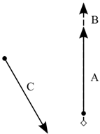
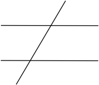
Qualitative spatial calculi usually deal with elementary objects (e.g. positions, directions, regions) and qualitative relations between them (e.g. 'adjacent', 'to the left of', 'included in'). This is the reason why qualitative descriptions are quite natural for people. The two main trends in Qualitative Spatial Reasoning (QSR) are topological reasoning about regions [3, 4, 5, 6, 7] and positional (e.g. direction and distance) reasoning about point configurations [8, 9, 10, 11, 12, 13, 14]. Positions can refer to a global reference system, e.g. cardinal directions, or just to local reference systems, e.g. egocentric views. Positional calculi can be related to the results of Psycholinguistic research [15] in the field of reference systems. In Psycholinguistics, local reference systems are divided into two modalities: intrinsic reference systems and extrinsic reference systems. Then, the three resulting options for giving a linguistic description of the spatial arrangements of objects are: intrinsic , extrinsic , and absolute (i.e. global) reference systems [16] 2 . Corresponding QSR calculi can be found in Psycholinguistics for all three types of reference systems. An intrinsic reference system employs an oriented physical object as the origin of a reference system (relatum). The orientation of the physical object then serves as a reference direction for the reference system. For instance, an intrinsic reference system is used in the calculus of oriented line segments (see Fig. 1) which is the main topic of this paper. Another calculus corresponding to intrinsic reference systems is the OPRA calculus [17]. In the OPRA calculus, oriented points are the basic entities (see Fig. 5).

Extrinsic reference systems are closely related to intrinsic reference systems. Both reference system options share the feature of focusing on the local context. The difference is that the extrinsic reference system superimposes the view direction from an external observer as reference direction to the relatum of the reference system. A typical example for a QSR calculus corresponding to an extrinsic reference system is Freksa's double cross calculus [18]. In the double cross calculus, two points span a reference system to localize a third point. The first point then projects a view towards the second point which generates the

1 Compare for example the qualitative expression 'one piece of material is longer than another' with the quantitative expression 'this thing is two meters long'

2 In [16], extrinsic references are called relative references.

reference direction.

Since intrinsic and extrinsic references are closely related in the rest of the paper, we sometimes refer to QSR calculi which use either intrinsic or extrinsic reference systems as relative position QSR calculi. Then, the two terms local reference systems and relative reference systems refer to the same concept. An interesting special case refers to the representation of a relative orientation without the concept of distance. These relative orientations can be viewed as decoupled from anchor points. Then there is no means for distinguishing between different point locations. The great advantage is that much more efficient reasoning mechanisms become available. The work by Isli and Cohn [19] consists of a ternary calculus for reasoning about such pure orientations. In contrast to relative position calculi, their algebra has a tractable subset containing the base relations.

Absolute (or global) directions can relate directional knowledge from distant places to each other. Cardinal directions as an example can be registered with a compass and compared over a large distance. And for that reason Frank's cardinal direction calculus corresponds to such an absolute reference system [9], [20]. There is a variant of a cardinal direction calculus, which has a flexible granularity, the Star Calculus [21].

In the previous paragraphs, we discussed the representation of spatial knowledge. Another important aspect are the reasoning mechanisms which are employed to make use of the represented initial knowledge to infer indirect knowledge. In Qualitative Spatial Reasoning two main reasoning modes are used: Conceptual neighbourhood-based reasoning, and constraint-based reasoning about (static) spatial configurations. Conceptual neighborhood-based reasoning describes whether two spatial configurations of objects can be transformed into each other by small changes [22]. The conceptual neighborhood of a qualitative spatial relation which holds for a spatial arrangement is the set of relations into which a relation can be changed with minimal transformations, e.g. by continuous deformation. Such a transformation can be a movement of one object in the configuration in a short period of time. At the discrete level of concepts, the neighborhood corresponds to continuity on the geometric or physical level of description: continuous processes map onto identical or neighboring classes of descriptions [23]. Spatial conceptual neighborhoods are very natural perceptual and cognitive entities and other neighborhood structures can be derived from spatial neighborhoods, e.g. temporal neighborhoods. The movement of an agent can then be modeled qualitatively as a sequence of neighboring spatial relations which hold for adjacent time intervals 3 . Based on this qualitative representation of trajectories, neighborhood-based spatial reasoning can for example be used as a simple, abstract model of the navigation of a spatial agent 4 .

In constraint-based reasoning about spatial configurations, typically a partial initial knowledge of a scene is represented in terms of qualitative constraints be-

3

This was the reasoning used in the first investigation of dipole relations by Schlieder [24] 4 for an application of neighbourhood based reasoning of spatial agents, we refer the reader to the simulation model SAILAWAY [25]

tween spatial objects. Implicit knowledge about spatial relations is then derived by constraint propagation 5 . Previous research has found that the mathematical notion of a relation algebra and related notions are well-suited for this kind of reasoning. In many cases, relation algebra-based reasoning only provides approximate results [26] and the constraint consistency problem for relative position calculi is NP-hard [27]. Hence we use constraint reasoning with polynomial time algorithms as an approximation of an intractable problem. The technical details of constraint reasoning are explained in Section 2.3.

In point-based reasoning, all objects are mapped onto the plane. The centers of projected objects can be used as point-like representation of the objects. By contrast, Schlieder's line segment calculus [24] uses more complex basic entities. Thus, it is based on extended objects which are represented as oriented straight line segments (see Fig. 1). These more complex basic entities capture important features of natural objects:

• Natural Objects are extended.
• Natural Objects often have an intrinsic direction.

Oriented straight line segments (which were called dipoles by Moratz et al. [28]) are the simplest geometric objects presenting these features. Dipoles may be specified by their start and end points.

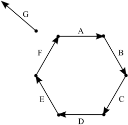
Using dipoles as basic blocks, more complex objects can be constructed (e.g. polylines, polygons) in a straightforward manner. Therefore, dipoles can be used as the basic units in numerous applications. To give an example, line segments are central to edge-based image segmentation and grouping in computer vision. In addition, GIS systems often have line segments as basic entities [29]. Polylines are particularly interesting for representing paths in cognitive robotics [30] and can serve as the geometric basis of a mobile robot when autonomously mapping its working environment [31].

The next sections of this paper present a detailed and technical description of dipole calculi. In Section 2 we introduce the relations of the dipole calculi

5 For an application of constraint-based reasoning for spatial agents, we refer the reader to the AIBO robot example in [14]

and revisit the theory of relation algebras and non-associate algebras underlying qualitative spatial reasoning. Furthermore, we investigate quotient of calculi on a general level as well as for the dipole calculi. Section 3 provides a condensed semantics for the dipole calculus. A condensed semantics, as we name it, provides spatial domain knowledge to the calculus in the form of an abstract symbolic model of a specific fragment of the spatial domain. In this model, possible configurations of very few of the basic spatial entities of a calculus are enumerated. In our case, we use orbits in the affine group GA ( R 2 ). This provides a useful abstraction for reasoning about qualitatively different configurations in Euclidean space. We use affine geometry at a rather elementary level and appeal to pictures instead of complete analytic arguments, whenever it is easy to fill in the details - however, at key points in the argument, careful analytic treatments are provided. Further, we calculate the composition tables for the dipole calculi using the condensed semantics and we investigate properties of the composition. In Section 4 we answer the question whether the standard constraint resoning method algebraic closure decides consistency for the dipole calculi. After the presentation of the technical details of dipole calculi and some of their properties, a sample application of dipole calculi using a spatial reasoning toolbox is presented in Section 5. The example uses the reasoning capabilities of a dipole calculus based on constraint reasoning. Our paper ends with a summary and conclusion and pointers to future work.

2 Representation of Dipole Relations and Relation Algebras

In this section, we first present a set of spatial relations between dipoles, then variants of this set of spatial relations. The final subsection shows mathematical structures for constraint reasoning about dipole relations.

2.1 Basic Representation of Dipole Relations

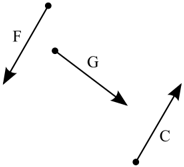
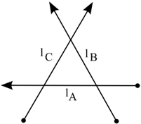
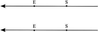
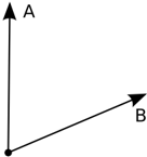
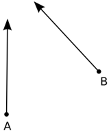
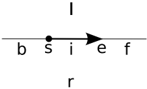
The basic entities we use are dipoles, i.e. oriented line segments formed by a pair of two points, a start point and an end point. Dipoles are denoted by A,B,C,... , start points by s A and end points by e A , respectively (see Fig. 1). These dipoles are used for representing spatial objects with an intrinsic orientation. Given a set of dipoles, it is possible to specify many different relations of different arity, e.g. depending on the length of dipoles, on the angle between different dipoles, or on the dimension and nature of the underlying space. When examining different relations, the goal is to obtain a set of jointly exhaustive and pairwise disjoint atomic or base relations, such that exactly one relation holds between any two dipoles. The elements of the powerset of the base relations are called general relations. These are used to express uncertainty about the relative position of dipoles. If these relations form an algebra which fulfills certain requirements, it is possible to apply standard constraint-based reasoning mechanisms that

were originally developed for temporal reasoning [32] and that have also proved valuable for spatial reasoning.

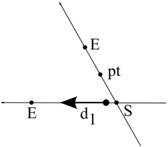
So as to enable efficient reasoning, an attempt should be made to keep the number of different base relations relatively small. For this reason, we will restrict ourselves to using two-dimensional continuous space for now, in particular R 2 , and distinguish the location and orientation of different dipoles only according to a small set of seven different dipole-point relations. We distinguish between whether a point lies to the left, to the right, or at one of five qualitatively different locations on the straight line that passes through the corresponding dipole 6 . The corresponding regions are shown on Fig. 2. A corresponding set of relations between three points was proposed by Ligozat [33] under the name flip-flop calculus and later extended to the LR calculus [34] 7 .

Then these dipole-point relations describe cases when the point is: to the left of the dipole (l); to the right of the dipole (r); straight behind the dipole (b); at the start point of the dipole (s); inside the dipole (i); at the end of the dipole (e); or straight in front of the dipole (f). For example, in Fig. 1, s B lies to the left of A , expressed as A l s B . Using these seven possible relations between a dipole and a point, the relations between two dipoles may be specified according to the following four relationships:

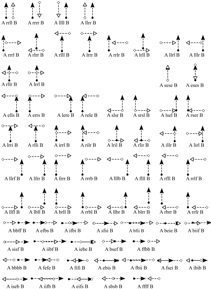
where R i ∈ { l , r , b , s , i , e , f } with 1 ≤ i ≤ 4. Theoretically, this gives us 2401 relations, out of which 72 relations are geometrically possible, see Prop. 47 below. They are listed on Fig. 3.

We introduce an operator that constructs a relation between two dipoles out of four dipole-point-relations:

6 In his introduction of a set of qualitative spatial relations between oriented line segments, Schlieder [24] mainly focused on configurations in which no more than two end or start points were on the same straight line (e.g. all points were in general position). However, in many domains, we may wish to represent spatial arrangements in which more than two start or end points of dipoles are on a straight line.

7 The LR calculus also features the relations dou and tri for both reference points or all points being equal, respectively. These cases are not possible for dipoles, since the start and end points cannot coincide by definition.

Definition 1. The operator glyph[rho1] takes the four LR relations between the start and end points of two dipoles and constructs a relation between dipoles. It is defined as the textual concatenation: glyph[rho1] (R 1 , R 2 , R 3 , R 4 ) = R 1 R 2 R 3 R 4 . By τ i with 1 ≤ i ≤ 4, we denote the projections to components of the relations between dipoles, where the identities glyph[rho1] ( τ 1 R , τ 2 R , τ 3 R , τ 4 R) = R and τ i ◦ glyph[rho1] (R 1 , R 2 , R 3 , R 4 ) = R i hold.

glyph[negationslash]

The relations that have been introduced above in an informal way can also be defined in an algebraic way. Every dipole D on the plane R 2 is an ordered pair of two points s D and e D , each of them being represented by its Cartesian coordinates x and y , with x, y ∈ R and s D = e D .

The basic relations are then described by equations with the coordinates as variables. The set of solutions for a system of equations describes all the possible coordinates for these points. One first such specification was presented in Moratz et. al. [28].

2.2 Several Versions of Sets of Dipole Base Relations

It is an unrealistic goal to provide a single set of qualitative base relations which is suitable for all possible contexts. In general, the desired granularity of a representation framework depends on the specific application [35]. A coarse granularity only needs a small set of base relations. Finer granularity can lead to a large number of base relations. If it is desired to apply a spatial calculus to a problem, it is therefore advantageous when a choice can be made between several versions of sets of base relations. Then a calculus may be selected which only has the necessary number of base relations and thus has less representation complexity but is fine-grained enough to solve the particular spatial reasoning problem. Focussing on the smallest number of base relations also fits better with the principle of a vocabulary of concepts which is compatible with linguistic principles [15, 14]. For this purpose, several versions of sets of dipole base relations can be constructed based on the base relation set of DRA f .

In their paper on customizing spatial and temporal calculi, Renz and Schmid [36] investigated different methods for deriving variants of a given calculus that have better-suited granularity for certain tasks. In the first variant, unions of base relations or so-called macro relations were used as base relations. In the second variant, only a subset of base relations was used as a new set of base relations. In his pioneering work on dipole relations, Schlieder [24] introduced a set of base relations in which no more than two start or end points were on the same straight line. As a result, only a subset of the DRA f base relations is used, which corresponds to Renz' and Schmid's second variant of methods for deriving new base relation sets for qualitative calculi. We refer to a calculus based on these base relations as DRA lr (where lr stands for left/right). The following base relations are part of DRA lr : rrrr, rrll, llrr, llll, rrrl, rrlr, rlrr, rllr, rlll, lrrr, lrrl, lrll, llrl, lllr.

{ llll , lllb , lllr , lrll , lbll } ↦→ LEFTleft { ffff , eses , fefe , fifi , ibib , fbii , fsei , ebis , iifb , eifs , iseb } ↦→ FRONTfront { bbbb } ↦→ BACKback { llbr } ↦→ LEFTback { llfl , lril , lsel } ↦→ LEFTfront { llrf , llrl , llrr , lfrr , lrrr , lere , lirl , lrri , lrrl } ↦→ LEFTright { rrrr , rrrl , rrrb , rbrr , rlrr } ↦→ RIGHTright { rrll , rrlr , rrlf , rlll , rfll , rllr , rele , rlli , rilr } ↦→ RIGHTleft { rrbl } ↦→ RIGHTback { rrfr , rser , rlir } ↦→ RIGHTfront { ffbb , efbs , ifbi , iibf , iebe } ↦→ FRONTback { frrr , errs , irrl } ↦→ FRONTright { flll , ells , illr } ↦→ FRONTleft { blrr } ↦→ BACKright { brll } ↦→ BACKleft { bbff , bfii , beie , bsef , biif } ↦→ BACKfront { slsr } ↦→ SAMEleft { sese , sfsi , sisf } ↦→ SAMEfront { sbsb } ↦→ SAMEback { srsl } ↦→ SAMEright

Moratz et al. [28] introduced an extension of DRA lr which adds relations for representing polygons and polylines. In this extension, two start or end points can share an identical location. While in this calculus, three points at different locations cannot belong to the same straight line. This subset of DRA f was named DRA c ( c refers to coarse , f refers to fine ). The set of base relations of DRA c extends the base relations of DRA lr with the following relations: ells, errs, lere, rele, slsr, srsl, lsel, rser, sese, eses.

Another method for deriving a new set of base relations from an existing set merges unions of base relations to new base relations. At a symbolic level, sets of base relations are used to form new base relations. In the context of DRA f , this is done as shown in Fig. 4 (the meaning of the names of the new base relations is explained in the following paragraphs).

DRA op is the name of the calculus which has the set of base relations listed

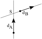
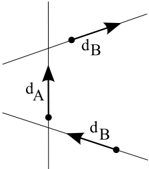
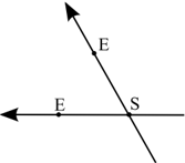
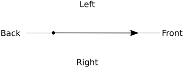
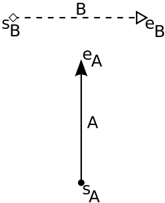
in Fig. 4. In [17], a calculus OPRA 1 which is isomorphic 8 to DRA op is defined in a complementary geometric way. The transition from oriented line segments with well-defined lengths to line segments with infinitely small lengths is the core idea of this geometric model. In this conceptualization, the length of objects no longer has any significance. Thus, only the direction of the objects is modeled [17]. These objects can then be conceptualized as oriented points. An o-point , our term for an oriented point, is specified as a pair of a point with a direction in the 2D-plane. Then the 'op' in the symbol DRA op stands for oriented points. A single o-point induces the sectors depicted in Fig. 5. 'Front' and 'Back' are linear sectors. 'Left' and 'Right' are half-planes. The position of the point itself is denoted as 'Same'. A qualitative spatial relative position relation between two o-points is represented by the sector in which the second o-point lies in relation to the first one and by the sector in which the first opoint lies in relation to the second one. For the general case of two points having different positions, we use the concatenated string of both sector names as the relation symbol. Then the configuration shown in Fig. 6 is expressed by the relation A RIGHTleft B . If both points share the same position, the relation symbol starts with the word 'Same' and the second substring denotes the direction of the second o-point relative to the first one as shown in Fig. 7.

8 Since we have not introduced operations on QSR calculi yet, we explain the details of the correspondence between DRA op and OPRA 1 later in our paper, see Prop. 21.

Altogether we obtain 20 different atomic relations (four times four general relations plus four with the oriented points at the same positions). The relation SAMEfront is the identity relation. DRA op has fewer base relations and therefore is more compact than DRA f . Focussing on a smaller set of base relations in this case also fits better with the principle of using a vocabulary of concepts which is compatible with linguistic principles [15, 14]. For this reason, many DRA op base relations have simple corresponding linguistic expressions. For example, the qualitative spatial configuration represented as A LEFTfront B can be translated into the natural language expression 'B is left of A and A is in front of B'. A and B in this example would be oriented objects with an intrinsic front like two cars A and B in a parking lot. However, in general, the correspondence between QSR expressions and their linguistic counterparts is only an approximation [15, 14].

The two methods for deriving new sets of base relations which we applied above reduce the number of base relations. Conversely, other methods extend the number of base relations. For example, Dylla and Moratz [37] have observed that DRA f may not be sufficient for robot navigation tasks, because the dipole configurations that are pooled in certain base relations are too diverse. Thus, the representation has been extended with additional orientation knowledge and a more fine-grained DRA fp calculus with additional orientation distinctions has been derived. It has slightly more base relations.

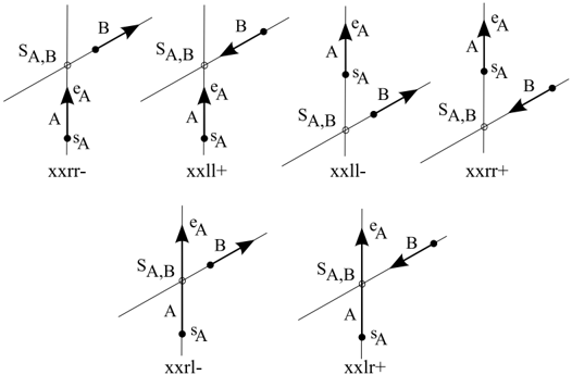
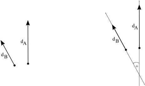
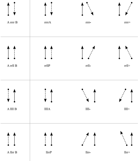
The large configuration space for the rrrr relation is visualized in Fig. 8. The other analogous relations which are extremely coarse are llrr, rrll and llll. In many applications, this unwanted coarseness of four relations can lead to problems 9 . Therefore, we introduce an additional qualitative feature by considering the angle spanned by the two dipoles. This gives us an important additional distinguishing feature with four distinctive values. These qualitative distinctions are parallelism (P) or anti-parallelism (A) and mathematically positive and negative angles between A and B , leading to three refining relations for each of the four above-mentioned relations (Fig. 9).

We call this algebra DRA fp as it is an extension of the fine-grained relation algebra DRA f with additional distinguishing features due to 'parallelism'. For the other relations, a '+' or ' -', 'P' or 'A' respectively, is already determined by the original base relation and does not have to be mentioned explicitly. These base relations then have the same relation symbol as in DRA f .

The introduction of parallelism into dipole calculi not only has benefits in certain applications. The algebraic features also benefit from this extension

9 An investigation by Dylla and Moratz into the first cognitive robotics applications of dipole relations integrated in situation calculus [37] showed that the coarseness of DRA f compared to DRA fp would indeed lead to rather meandering paths for a spatial agent.

(see Sect. 3.7). For analogous reasons, a derivation of DRA fp yields an oriented point calculus which explicitly contains the feature of parallelism, which is isomorphic to the OPRA ∗ 1 calculus[38]. This calculus DRA opp (opp stands for oriented points and parallelism) has the same base relations as DRA op with the exception of the relations RIGHTright, RIGHTleft, LEFTleft, and LEFTright. The transformation from DRA fp to DRA opp is shown in Fig. 10.

Again, the mathematical properties of the oriented point calculus can be derived from the corresponding dipole calculus, see Corollary 55.

2.3 Relation Algebras for Spatial Reasoning

Standard methods developed for finite domains generally do not apply to constraint reasoning over infinite domains. The theory of relation algebras [39, 40] allows for a purely symbolic treatment of constraint satisfaction problems involving relations over infinite domains. The corresponding constraint reasoning techniques were originally introduced for temporal reasoning [32] and later proved to be valuable for spatial reasoning [6, 19]. The central data for a calculus is given by:

• a list of (symbolic names for) base relations , which are interpreted as relations over some domain, having the crucial properties of pairwise disjointness and joint exhaustiveness (a general relation is then simply a set of base relations).
• a table for the computation of the converses of relations.
• a table for the computation of the compositions of relations.

Then, the path consistency algorithm [41] and backtracking techniques [42] are the tools used to tackle the problem of consistency of constraint networks and related problems. These algorithms have been implemented in both generic reasoning tools GQR [43] and SparQ [44]. To integrate a new calculus into these tools, only a list of base relations and tables for compositions and converses really need to be provided. Thereby, the qualitative reasoning facilities of these tools become available for this calculus. 10 Since the compositions and converses of general relations can be reduced to compositions and converses of base relations, these tables only need to be given for base relations. Based on these tables, the tools provide a means to approximate the consistency of constraint networks, list all their atomic refinements, and more.

Let b be the name of a base relation, and let R b be its set-theoretic extension. The converse ( R b ) glyph[smile] = { ( x, y ) | ( y, x ) ∈ R b } is often itself a base relation and is denoted by b glyph[smile] 11 . In the dipole calculus, it is obvious that the converse of a relation can easily be computed by exchanging the first two and second two

10 With more information about a calculus, both of the tools can provide functionality that goes beyond simple qualitative reasoning for constraint calculi.

11 In Freksa's double-cross calculus [2] the converses are not necessarily base-relations, but for the calculi that we investigate this property holds.

Table 1: The converse ( glyph[slurbelow] ) operation of DRA f can be reduced to a simple permutation.

R	rrrr	rrrl	rrlr	rrll	rlrr	rllr	rlll	lrrr
R glyph[slurbelow]	rrrr	rlrr	lrrr	llrr	rrrl	lrrl	llrl	rrlr

letters of the name of a relation, see Table 1. Also for the dipole calculus DRA fp with additional orientation distinctions a simple rule exchanges '+' with ' -', and vice versa.'P' and 'A' are invariant with respect to the converse operation. Since base relations generally are not closed under composition, this operation is approximated by a weak composition :

glyph[negationslash]

where R b 1 ◦ R b 2 is the usual set theoretic composition

The composition is said to be strong if R b 1 ; b 2 = R b 1 ◦ R b 2 . Generally, b 1 ; b 2 over-approximates the set-theoretic composition. 12 Computing the composition table is much harder and will be the subject of Section 3.

The mathematical background of composition in table-based reasoning is given by the theory of relation algebras [40, 45]. For many calculi, including the dipole calculus, a slightly weaker notion is needed, namely that of a nonassociative algebra [46]. These algebras treat spatial relations as abstract entities that can be combined by certain operations and governed by certain equations. This allows algorithms and tools to operate at a symbolic level, in terms of (sets of) base relations instead of their set-theoretic extensions.

Definition 2 ([46]) . A non-associative algebra A is a tuple A = ( A, + , -, · , 0 , 1 , ; , glyph[smile] , ∆) such that:

1. ( A, + , -, · , 0 , 1) is a Boolean algebra.
2. ∆ is a constant, glyph[smile] a unary and ; a binary operation such that, for any a, b, c ∈ A :

A non-associative algebra is called a relation algebra , if the composition ; is associative.

The elements of such an algebra will be called (abstract) relations. We are mainly interested in finite non-associative algebras that are atomic , which means

12 The R operation naturally extends to sets of (names of) base relations.

that there is a set of pairwise disjoint minimal relations, called base relations, and all relations can be obtained as unions of base relations. Then, the following fact is well-known and easy to prove:

Proposition 3. An atomic non-associative algebra is uniquely determined by its set of base relations, together with the converses and compositions of base relations. (Note that the composition of two base relations is in general not a base relation.)

Example 4. The powerset of the 72 DRA f base relations forms a boolean algebra. The relation sese is the identity relation. The converse and (weak) composition are defined as above. We denote the resulting non-associative algebra by DRA f . The algebraic laws follow from general results about so-called partition schemes, see [46]. Similarly, we obtain a non-associative algebra DRA fp .

However, we do not obtain a non-associative algebra for DRA c , because DRA c does not provide a jointly exhaustive set of base relations over the Euclidean plane. This leads to the lack of an identity relation, and more severely, weak composition does not lead to an over-approximation (nor an under-approximation) of set-theoretic composition, because e.g. ffbb is missing from the composition of llll with itself. In particular, we cannot expect the algebraic laws of a non-associative algebra to be satisfied.

For non-associative algebras, we define lax homomorphisms which allow for both the embedding of a calculus into another one, and the embedding of a calculus into its domain.

Definition 5 (Lax homomorphism) . Given non-associative algebras A and B , a lax homomorphism is a homomorphism h : A -→ B on the underlying Boolean algebras such that:

• h(∆ A ) ≥ ∆ B
• h( a glyph[slurbelow] ) = h( a ) glyph[slurbelow] for all a ∈ A
• h( a ; b ) ≥ h( a ); h( b ) for all a, b ∈ A

Dually to lax homomorphisms, we can define oplax homomorphisms 13 , which enable us to define projections from one calculus to another.

Definition 6 (Oplax homomorphism) . Given non-associative algebras A and B , an oplax homomorphism is a homomorphism h : A -→ B on the underlying Boolean algebras such that:

• h(∆ A ) ≤ ∆ B
• h( a glyph[slurbelow] ) = h( a ) glyph[slurbelow] for all a ∈ A
• h( a ; b ) ≤ h( a ); h( b ) for all a, b ∈ A

13 The terminology is motivated by that for monoidal functors.

A proper homomorphism (sometimes just called a homomorphism) of nonassociative algebras is a homomorphism that is lax and oplax at the same time; the above inequalities then turn into equations.

An important application of homomorphisms is their use in the definition of qualitative calculus. Ligozat and Renz [46] define a qualitative calculus in terms of a so-called weak representation [47]:

Definition 7 (Weak representation) . A weak representation is an identitypreserving (i.e. h(∆ A ) = ∆ B ) lax homomorphism ϕ from a (finite atomic) nonassociative algebra into the relation algebra of a domain U . The latter is given by the canonical relation algebra on the powerset P ( U × U ), where identity, converse and composition (as well as the Boolean algebra operations) are given by their set-theoretic interpretations.

Example 8. Let D be the set of all dipoles in R 2 . Then the weak representation of DRA f is the lax homomorphism ϕ f : DRA f →P ( D × D ) given by

We obtain a similar weak representation ϕ fp for DRA fp . The following is straightforward:

Proposition 9. A calculus has a strong composition if and only if its weak representation is a proper homomorphism.

Proof. Since a weak representation is identity-preserving, being proper means that ϕ ( R 1 ; R 2 ) = ϕ ( R 1 ) ◦ ϕ ( R 2 ), which is nothing but R R 1 ; R 2 = R R 1 ◦ R R 2 , which is exactly the strength of the composition.

The following is straightforward [47]:

Proposition 10. A weak representation ϕ is injective if and only if ϕ ( b ) = ∅ for each base relation b .

glyph[negationslash]

The second main use of homomorphisms is relating different calculi. For example, the algebra over Allen's interval relations [32] can be embedded into DRA f ( DRA fp ) via a homomorphism.

Proposition 11. A homomorphism from Allen's interval algebra to DRA f ( DRA fp ) exists and is given by the following mapping of base relations.

=	↦→	sese
b	↦→	ffbb	bi	↦→	bbff
m	↦→	efbs	mi	↦→	bsef
o	↦→	ifbi	oi	↦→	biif
d	↦→	bfii	di	↦→	iibf
s	↦→	sfsi	si	↦→	sisf
f	↦→	beie	fi	↦→	iebe

Proof. The identity relation = is clearly mapped to the identity relation sese. For the composition and converse properties, we just inspect the composition and converse tables for the two calculi. 14 The mapping of the base-relation is then lifted directly to a mapping of all relations, where the map is applied component-wise on the relations. Using the laws of non-associative algebras, the homomorphism property of these relations follows from that of the baserelations.

In cases stemming from the embedding of Allen's Interval Algebra, the dipoles lie on the same straight lines and have the same direction. DRA f and DRA fp also contain 13 additional relations which correspond to the case with dipoles lying on a line but facing opposite directions.

As we shall see, it is very useful to extend the notion of homomorphisms to weak representations:

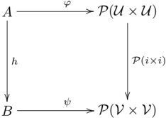
Definition 12. Given weak representations ϕ : A → P ( U × U ) and ψ : B → P ( V × V ), a lax (oplax, proper) homomorphism of weak representations ( h, i ) : ϕ → ψ is given by

• a proper homomorphism of non-associative algebras h : A → B , and
• a map i : U → V , such that the diagram

/

/

GLYPH<15>

GLYPH<15>

GLYPH<15>

GLYPH<15>

/

/

commutes laxly (respectively oplaxly, properly). Here, lax commutation means that for all R ∈ A , ψ ( h ( R )) ⊆ P ( i × i )( ϕ ( R )), oplax commutation means the same with ⊇ , and proper commutation with =. Note that P ( i × i ) is the obvious extension of i to a function between relation algebras; note that (unless i is bijective) this is not even a homomorphism of Boolean algebras (it may fail to preserve top, intersections and complements), although it satisfies the oplaxness property (and the laxness property if i is surjective). 15

Note that Ligozat [47] defines a more special notion of morphism between weak representations; it corresponds to our oplax homomorphism of weak representations where the component h is the identity.

14 This is a (non-circular) forward reference to Section 3, where we compute the DRA f and DRA fp composition tables.

15 The reader with background in category theory may notice that the categorically more natural formulation would use the contravariant powerset functor, which yields homomorphisms of Boolean algebras. However, the present formulation fits better with the examples.

Example 13. The homomorphism from Prop. 11 can be extended to a proper homomorphism of weak representations by letting i be the embedding of time intervals to dipoles on the x -axis.

Example 14. Let h map each DRA fp relation to the corresponding DRA f relation:

llll+ ↦→ llll llll-↦→ llll llllA ↦→ llll rrrr+ ↦→ rrrr rrrr-↦→ rrrr rrrrA ↦→ rrrr llrr+ ↦→ llrr llrr-↦→ llrr llrrP ↦→ llrr rrll+ ↦→ rrll rrll-↦→ rrll rrllP ↦→ rrll

Then ( h, id ) : DRA fp → DRA f is a surjective oplax homomorphism of weak representations.

Although this homomorphism of weak representations is surjective, it is not a quotient in the following sense (and in particular, it does not satisfy Prop. 20, as will be shown in Sections 3.8 and 3.9).

Definition 15. A homomorphism of non-associative algebras is said to be a quotient homomorphism 16 if it is proper and surjective. A (lax, oplax or proper) homomorphism of weak representations is a quotient homomorphism if it is surjective in both components.

The easiest way to form a quotient of a weak representation is via an equivalence relation on the domain:

Definition 16. Given a weak representation ϕ : A →P ( U × U ) and an equiv-

16 Maddux [40] does not have much to say on this subject; instead, we suggest consulting a textbook on universal algebra, e.g. [48].

alence relation ∼ on U , we obtain the quotient representation ϕ/ ∼ as follows:

/

/

GLYPH<15>

GLYPH<15>

GLYPH<15>

GLYPH<15>

/

/

• Let q : U → U / ∼ be the factorization of U by ∼ ;
• q extends to relations: P ( q × q ) : P ( U × U ) →P ( U / ∼ ×U / ∼ );
• let ∼ A be the congruence relation on A generated by

glyph[negationslash]

for base relations b 1 , b 2 ∈ A . ∼ is called regular w.r.t. ϕ if ∼ A is the kernel of P ( q × q ) ◦ ϕ (i.e. the set of all pairs made equal by P ( q × q ) ◦ ϕ );

• let q A : A → A/ ∼ A be the quotient of A by ∼ A in the sense of universal algebra [48], which uses proper homomorphisms; hence, q A is a proper homomorphism;
• finally, the function ϕ/ ∼ is defined as

Proposition 17. The function ϕ/ ∼ defined in Def. 16 is an oplax homomorphism of non-associative algebras.

Proof. To show this, notice that an equivalent definition works on the base relations of A/ ∼ A :

It is straightforward to show that bottom and joins are preserved; since q is surjective, also top is preserved.

glyph[negationslash]

Concerning meets, since general relations in A/ ∼ A can be considered to be sets of base relations, it suffices to show that b 1 ∧ b 2 = 0 implies P ( q × q )( ϕ ( q -1 A ( b 1 ))) ∩ P ( q × q )( ϕ ( q -1 A ( b 2 ))) = ∅ . Assume to the contrary that P ( q × q )( ϕ ( q -1 A ( b 1 ))) ∩ P ( q × q )( ϕ ( q -1 A ( b 2 ))) = ∅ . Then already P ( q × q )( ϕ ( b ′ 1 )) ∩ P ( q × q )( ϕ ( b ′ 2 )) = ∅ for base relations b ′ i ∈ q -1 A ( b i ), i = 1 , 2. But then b ′ 1 ∼ A b ′ 2 , hence q A ( b ′ 1 ) = q A ( b ′ 2 ) ≤ b 1 ∧ b 2 , contradicting b 1 ∧ b 2 = 0. Preservation of complement follows from this.

glyph[negationslash]

Using properness of the quotient, it is then easily shown that the relation algebra part of the lax homomorphism property carries over from ϕ to ϕ/ ∼ : Concerning composition, by surjectivity of q A , we know that any given relations R 1 , R 2 ∈ A/ ∼ A are of the form R 1 = q A ( S 1 ) and R 2 = q A ( S 2 ). Hence, ϕ/ ∼ ( R 1 ; R 2 ) = ϕ/ ∼ ( q A ( S 1 ); q A ( S 2 )) = ϕ/ ∼ ( q A ( S 1 ; S 2 )) = P ( q × q )( ϕ ( S 1 ; S 2 )) ≥ P ( q × q )( ϕ ( S 1 ); ϕ ( S 2 )) = P ( q × q )( ϕ ( S 1 )); P ( q × q )( ϕ ( S 2 )) = ϕ/ ∼ ( q A ( S 1 )); ϕ/ ∼ ( q A ( S 2 )) = ϕ/ ∼ ( R 1 ); ϕ/ ∼ ( R 2 ). The inequality of the identity is shown similarly.

Proposition 18. ( q A , q ) : ϕ → ϕ/ ∼ is an oplax quotient homomorphism of weak representations. If ∼ is regular w.r.t. ϕ , then the quotient homomorphism is proper, and satisfies the following universal property: if ( q B , i ) : ϕ → ψ is another oplax homomorphism of weak representations with ψ injective and ∼⊆ ker ( i ) , then there is a unique oplax homomorphism of weak representations ( h, k ) : ϕ/ ∼→ ψ with ( q B , i ) = ( h, k ) ◦ ( q A , q ) .

Proof. The oplax homomorphism property for ( q A , q ) is P ( q × q ) ◦ ϕ ⊆ ϕ/ ∼ ◦ q A , which by definition of ϕ/ ∼ amounts to

which follows from surjectivity of q . Regularity of ∼ is w.r.t. ϕ means that ∼ A is the kernel of P ( q × q ) ◦ ϕ , which turns the above inequation into an equality. Concerning the universal property, let ( q B , i ) : ϕ → ψ with the mentioned properties be given. Since ∼⊆ ker ( i ), there is a unique function k : U / ∼→ V with i = k ◦ q . The homomorphism h we are looking for is determined uniquely by h ( q A ( b )) = q B ( b ); this also ensures the proper homomorphism property. All that remains to be shown is well-definedness. Suppose that b 1 ∼ A b 2 . By regularity, P ( q × q )( ϕ ( b 1 )) = P ( q × q )( ϕ ( b 2 )). Hence also P ( i × i )( ϕ ( b 1 )) = P ( i × i )( ϕ ( b 2 )) and ψ ( q B ( b 1 )) = ψ ( q B ( b 2 )). By injectivity of ψ , we get q B ( b 1 ) = q B ( b 2 ).

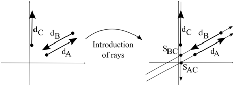
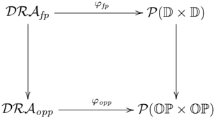
Example 19. Given dipoles d 1 , d 2 ∈ D , let d 1 ∼ d 2 denote that d 1 and d 2 have the same start point and point in the same direction. (This is regular w.r.t. ϕ f .) Then D / ∼ is the domain OP of oriented points in R 2 . Let ϕ op : DRA op → P ( OP × OP ) and ϕ opp : DRA opp →P ( OP × OP ) be the weak representations obtained as quotients of ϕ f and ϕ fp , respectively, see Fig. 11. At the level of non-associative algebras, the quotient is given by the tables in Figs. 4 and 10.

This way of constructing DRA op and DRA opp by a quotient gives us their converse and composition tables for no extra effort; we can obtain them by applying the respective congruences to the tables for DRA f and DRA fp , respectively. Moreover, the next result shows that we also can use the quotient to transfer an important property of calculi.

Proposition 20. Quotient homomorphism of weak representations preserve strength of composition.

Proof. Let ( h, i ) : ϕ → ψ with ϕ : A →P ( U × U ) and ψ : B →P ( V × V ) be a quotient homomorphism of weak representations. According to Prop. 9, the

strength of the composition is equivalent to ϕ (respectively ψ ) being a proper homomorphism. We assume that ϕ is a proper homomorphism and need to show that ψ is proper as well. We also know that h and P ( i × i ) are proper. Let R 2 , S 2 be two abstract relations in B . Because of the surjectivity of h , there are abstract relations R 1 , S 1 ∈ A with h ( R 1 ) = R 2 and h ( S 1 ) = S 2 . Now ψ ( R 2 ; S 2 ) = ψ ( h ( R 1 ); h ( S 1 )) = ψ ( h ( R 1 ; S 1 )) = P ( i × i )( ϕ ( R 1 ; S 1 )) = P ( i × i )( ϕ ( R 1 )); P ( i × i )( ϕ ( S 1 )) = ψ ( h ( R 1 )); ψ ( h ( S 1 )) = ψ ( R 2 ); ψ ( S 2 ), hence ψ is proper.

The application of this Proposition must wait until Section 3, where we develop the necessary machinery to investigate the strength of the calculi. The domains of DRA op and OPRA 1 obviously coincide. An inspection of the converse and composition tables (that of OPRA 1 is given in [49]) shows:

Proposition 21. DRA op is isomorphic to OPRA 1 .

We can also obtain a similar statement for DRA opp . The calculus OPRA ∗ 1 [38] is a refinement of OPRA 1 that is obtained along the same features as DRA fp is obtained from DRA f . The method how to compute the composition table for OPRA ∗ 1 is described in [38] and a reference composition table is provided with the tool SparQ [50].

Proposition 22. DRA opp is isomorphic to OPRA ∗ 1 .

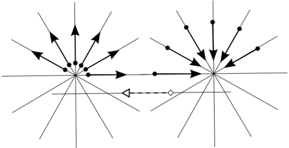
In the course of checking the isomorphism properties between DRA opp and OPRA ∗ 1 , we discovered errors in 197 entries of the composition table of OPRA ∗ 1 as it was shipped with the qualitative reasoner SparQ [50]. This emphasizes our point how important it is to develop a sound mathematical theory to compute a composition table and to stay as close as possible with the implementation to the theory. In the composition table for OPRA ∗ 1 it was claimed that

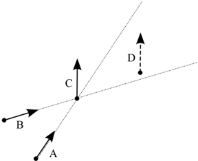
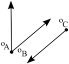
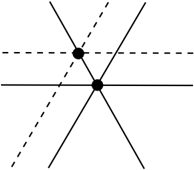
SAMEright;RIGHTrightA = ⇒ { LEFTright+ , LEFTrightP , LEFTright-, BACKright , RIGHTright+ , RIGHTrightA , RIGHTright-}

were we use the DRA opp notation for the OPRA ∗ 1 -relations for convenience. So the abstract composition SAMEright; RIGHTrightA contains the base relation LEFTrightP, which however is not supported geometrically. Consider three oriented points o A , o B and o C with o A SAMEright o B and o B RIGHTrightA o C , as depicted in Fig. 12. For the relation o A LEFTrightP o C to hold, the carrier rays of o A and o C need to be parallel, but because of o B RIGHTrightA o C , the carrier rays of o B and o C and hence also those of o A and o B need to be parallel as well. Since the start point of o A and o B coincide, this can only be achieved, if o A and o B are collinear, which is a contradiction to o A SAMEright o B .

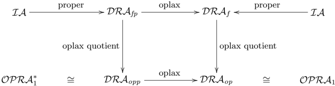
Altogether, we get the following diagram of calculi (weak representations) and homomorphisms among them:

/

/

/

/

o

o

GLYPH<15>

GLYPH<15>

2.4 Constraint Reasoning

Let us now apply the relation-algebraic method to constraint reasoning. Dipole constraints are written as xRy , where x, y are variables for the dipoles and R is a DRA f or DRA fp relation. Given a set Θ of dipole constraints, an important reasoning problem is to decide whether Θ is consistent , i.e., whether there is an assignment of all variables of Θ with dipoles such that all constraints are satisfied (a solution ). We call this problem DSAT . DSAT is a Constraint Satisfaction Problem (CSP) [51]. We rely on relation algebraic methods to check consistency, namely the above mentioned path consistency algorithm. For non-associative algebras, the abstract composition of relations need not coincide with the (associative) set-theoretic composition. Hence, in this case, the standard path-consistency algorithm does not necessarily lead to path consistent networks, but only to algebraic closure [26]:

Definition 23 (Algebraic Closure) . A CSP over binary relations is called algebraically closed if for all variables X 1 , X 2 , X 3 and all relations R 1 , R 2 , R 3 the constraint relations

imply

In general, algebraic closure is therefore only a one-sided approximation of consistency: if algebraic closure detects an inconsistency, then we are sure that the constraint network is inconsistent; however, algebraic closure may fail to detect some inconsistencies: an algebraically closed network is not necessarily consistent. For some calculi, like Allen's interval algebra, algebraic closure is known to exactly decide consistency, for others it does not, see [26], where it is also shown that this question is completely orthogonal to the question as to whether the composition is strong. We will examine these questions for the dipole calculi in Section 3 below.

Fortunately, it turns out that oplax homomorphisms preserve algebraic closure.

/

/

GLYPH<15>

GLYPH<15>

Proposition 24. Given non-associative algebras A and B , an oplax homomorphism h : A -→ B preserves algebraic closure. If h is injective, it also reflects algebraic closure.

Proof. Since an oplax homomorphism is a homomorphism between Boolean algebras, it preserves the order. So for any three relations R 1 , R 2 , R 3 in the algebraically closed CSP over A , with

the preservation of the order implies:

Applying the oplaxness property yields:

and hence the image of the CSP under h is also algebraically closed. If h is injective, it reflects equations and inequations, and the converse implication follows.

Definition 25. Following [26], a constraint network over a non-associative algebra A can be seen as a function ν : A → P ( N × N ), where N is the set of nodes (or variables), and ν maps each abstract relation R to the set of pairs ( n 1 , n 2 ) that are decorated with R . (Note that ν is a weak representation only if the constraint network is algebraically closed.)

Constraint networks can be translated along homomorphisms of nonassociative algebras as follows: Given h : A → B and ν : A → P ( N × N ), h ( ν ) : B →P ( N × N ) is the network that decorates ( n 1 , n 2 ) with h ( R ) whenever ν decorates it with R

A solution for ν in a weak representation ϕ : A → P ( U × U ) is a function j : N →U such that for all R ∈ A , P ( j × j )( ν ( R )) ⊆ ϕ ( R ), or P ( j × j ) ◦ ν ⊆ ϕ for short.

Proposition 26. Oplax homomorphisms of weak representations preserve solutions for constraint networks.

Proof. Let weak representations ϕ : A →P ( U × U ) and ψ : B →P ( V × V ) and an oplax homomorphism of weak representations ( h, i ) : ϕ → ψ be given.

A given solution j : N → U for ν in ϕ is defined by P ( j × j ) ◦ ν ⊆ ϕ . From this and the oplax commutation property P ( i × i ) ◦ ϕ ⊆ ψ ◦ h we infer P ( i ◦ j × i ◦ j ) ◦ ν ⊆ ψ ◦ h , which implies that i ◦ j is a solution for h ( ν ).

An important question for a calculus (= weak representation) is whether algebraic closure decides consistency. We will now prove that this property is preserved under certain homomorphisms.

Proposition 27. Oplax homomorphisms ( h, i ) of weak representations with h injective preserve the property that algebraic closure decides consistency to the image of h .

Proof. Let weak representations ϕ : A →P ( U × U ) and ψ : B →P ( V × V ) and an oplax homomorphism of weak representations ( h, i ) : ϕ → ψ be given. Further assume that for ϕ , algebraic closure decides consistency.

Any constraint network in the image of h can be written as h ( ν ) : B → P ( N × N ). If h ( ν ) is algebraically closed, by Prop. 24, this carries over to ν . Hence, by the assumption, ν is consistent, i.e. has a solution. By Prop. 26, h ( ν ) is consistent as well. Note that the converse directly always holds: any consistent network is algebraically closed.

For calculi such as RCC8, interval algebra etc., (maximal) tractable subsets have been determined, i.e. sets of relations for which algebraic closure decides consistency. We can apply Prop. 27 to the homomorphism from interval algebra to DRA f (see Example 13). We obtain that algebraic closure in DRA f decides consistency of any constraint network involving (the image of) a maximal tractable subset of the interval algebra only.

On the other hand, the consistency problem for the DRA c calculus in the base relations is already NP-hard, see [27], and hence algebraic closure does not decide consistency in this case. We will resume the discussion of consistency versus algebraic closure in Sect. 4.

3 A Condensed Semantics for the Dipole Calculus

The 72 base relations of DRA f , or the 80 base relations of DRA fp , have so far been derived manually. This is a potentially erroneous procedure 17 , especially if the calculus has many base-relations like the DRA f and DRA fp calculi. Therefore, it is necessary to use methods which yield more reliable results. To start, we tried verifying the composition table of DRA f directly, using the resulting quadratic inequalities as given in [28]. However, it turned out that it is unfeasible to base the reasoning on these inequalities, even with the aid of interactive theorem provers such as Isabelle/HOL [52] and HOL-light [53] (the latter is dedicated to proving facts about real numbers). This unfeasibility is probably related to the above-mentioned NP-hardness of the consistency problem for DRA f base relations. So, we developed a qualitative abstraction instead. A key insight is that two configurations are qualitatively different if they cannot be transformed into each other by maps that keep that part of the spatial structure invariant that is essential for the calculus. In our case, these maps are (orientation-preserving) affine bijections. A set of configurations that can

17 For this reason, the manually derived sets of base relations for the finer-grained dipole calculi described in [24, 28] contained errors.

be transformed into each other by appropriate maps is an orbit of a suitable automorphism group. Here, we use primarily the affine group GA ( R 2 ) and detail how this leads to qualitatively different spatial configurations.

3.1 Seven qualitatively different configurations

Since the domains of most spatial calculi are infinite (e.g. the Euclidean plane), it is impossible just to enumerate all possible configurations relative to the composition operation when deriving a composition table. It is still possible to enumerate a well-chosen subset of all configurations to obtain a composition table, but it is difficult to show that this subset leads to a complete table. We have experimented with the enumeration of all DRA f scenarios with six points (which are the start- and end-points of three dipoles), which are equivalent to the entries of the composition table, in a finite grid over natural numbers. This method led to a usable composition table, but its computation took several weeks and it is unclear if it is complete. The goal remains the efficient and automatic computation of a composition table. To obtain an efficient method for computing the table, we introduce the condensed semantics for DRA f and DRA fp . For these, we observe the Euclidean plane with respect to all possible line configurations that are distinguishable within the DRA calculi. With condensed semantics, there is already a level of abstraction from the metrics of the underlying space. All we can see are lines that are parallel or intersect. For the binary composition operation of DRA calculi, we have to consider all qualitatively different configurations of three lines.

In order to formalize 'qualitatively different configurations', we regard the DRA calculus as a first-order structure, with the Euclidean plane as its domain, together with all the base relations.

Proposition 28. All orientation-preserving affine bijections are DRA f and DRA fp automorphisms.

(In [54], the converse is also shown.)

Proof. It suffices to show that orientation preserving affine bijections preserve the LR relations. Now, any orientation-preserving affine bijection can be composed of translations, rotations, scalings and shears. It is straightforward to see that these mappings preserve the LR relations.

Recall that an affine map f from Euclidean space to itself is given by

f is a bijection iff det ( A ) is non-zero.

Automorphisms and their compositions form a group which acts on the set of points (and tuples of points, lines, etc.) by function application. Recall that, if a group G acts on a set, an orbit consists of the set reachable from a fixed

element by performing the action of all group elements: O ( x ) = { f ( x ) | f ∈ G } . The importance of this notion is the following:

Qualitatively different configurations are orbits of the automorphism group.

Here, we start with configurations consisting of three lines, i.e. we consider the orbits for all sets { l 1 , l 2 , l 3 } of (at most) three lines 18 in Euclidean space with respect to the group of all affine bijections (and not just the orientation preserving ones - orientations will come in at a later stage). This group is usually called the affine group of R 2 and denoted by GA ( R 2 ).

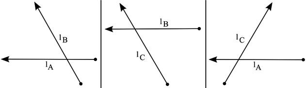
A line in Euclidean space is given by the set of all points ( x, y ) for which y = mx + b . Given three lines y = m i x + b i ( i = 1 , 2 , 3), we list their orbits by giving a defining property. In each case, it is fairly obvious that the defining property is preserved by affine bijections. Moreover, in each case, we show a transformation property , namely that given two instances of the defining properties, the first can be transformed into the second by an affine bijection. Together, this means that the defining property exactly specifies an orbit. The transformation property often follows from the following basic facts about affine bijections, see [55]:

1. An affine bijection is uniquely determined by its action on an affine basis, the result of which is given by another affine basis. Since an affine basis of the Euclidean plane is a point triple in general position, given any two point triples in general position, there is a unique affine bijection mapping the first point triple to the second.
2. Affine maps transform lines into lines.
3. Affine maps preserve parallelism of lines.

That is, it suffices to show that an instance of the defining property is determined by three points in general position and drawing lines and parallel lines.

glyph[negationslash]

We will consider the intersection of line i with line j ( i = j ∈ { 1 , 2 , 3 } ). This is given by the system of equations:

For m i = m j , this has a unique solution:

glyph[negationslash]

For m i = m j , there is either is no solution ( b i = b j ; the lines are parallel), or there are infinitely many solutions ( b i = b j ; the lines are identical).

We can now distinguish seven cases:

18 We do not require that l 1 , l 2 and l 3 are distinct; hence, the set { l 1 , l 2 , l 3 } may also consist of two elements or be a singleton.

glyph[negationslash]

glyph[negationslash]

1. All m i are distinct and the three systems of equations { y = m i x + b i , y = m j x + b j } ( i = j ∈ { 1 , 2 , 3 } ) yield three different solutions. Geometrically, this means that all three lines intersect with three different intersection points. The transformation property follows from the fact that the three intersection points determine the configuration.

glyph[negationslash]

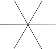
1. All m i are distinct and at least two of the three systems of equations { y = m i x + b i , y = m j x + b j } ( i = j ∈ { 1 , 2 , 3 } ) have a common solution. Then, obviously, the single solution is common to all three equation systems. Geometrically, this means that all three lines intersect at the same point.

Take this point and a second point on one of the lines. By drawing parallels through this second point, we obtain two more points, one on each of the other two lines, such that the four points form a parallelogram. The transformation property now follows from the fact that any two nondegenerate parallelograms can be transformed into each other by an affine bijection.

glyph[negationslash]

glyph[negationslash]

An affine bijection glyph[negationslash]

1. m i = m j = m k and b i = b j for distinct i, j, k ∈ { 1 , 2 , 3 } . Geometrically, this means that two lines are parallel, but not coincident, and the third line intersects them. Such a configuration is determined by three points: the points of intersection, plus a further point on one of the parallel lines. Hence, the transformation property follows.
2. m i = m j = m k and b i = b j for distinct i, j, k ∈ { 1 , 2 , 3 } . Geometrically, this means that two lines are equal and a third one intersects them. Again, such a configuration is determined by three points: the intersection point plus a further point on each of the (two) different lines. Hence, the transformation property follows.
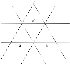
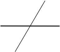
3. All m i are equal, but the b i are distinct. Geometrically, this means that all three lines are parallel, but not coincident. We cannot show the transformation property here, which means that this case comprises several orbits. Actually, we get one orbit for each distance ratio

transforms a line y = mx + b to y = m ′ x + b ′ , with b ′ = c 1 ( m ) b + c 2 ( m ), where c 1 and c 2 depend non-linearly on m . However, since m = m 1 = m 2 = m 3 , this non-linearity does not matter. This means that

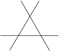
i.e. the distance ratio is invariant under affine bijections (which is wellknown in affine geometry). Given a fixed distance ratio, we can show the transformation property: three points suffice to determine two parallel lines, and the position of the third parallel line is then determined by the distance ratio. For a distance ratio 1, this configuration looks as follows:

Actually, for the qualitative relations between dipoles placed on parallel lines, their distance ratio does not matter. Hence, we will ignore distance ratios when computing the composition table below. The fact that we get infinitely many orbits for this sub-case will be discussed below.

1. All m i are equal and two of the b i are equal but different from the third. Geometrically, this means that two lines are coincident, and a third one is parallel but not coincident. Such a configuration is determined by three points: two points on the coincident lines and a third point on the third line. Hence, the transformation property follows.
2. All m i are equal, and the b i are equal as well. This means that all three lines are equal. The transformation property is obvious.

Since we have exhaustively distinguished the various possible cases based on relations between the m i and b i parameters, this describes all possible orbits of three lines w.r.t. affine bijections. Although we get infinitely many orbits for case (5), in contexts where the distance ratio introduced in case (5) does

not matter, we will speak of seven qualitatively different configurations, and it is understood that the infinitely many orbits for case (5) are conceptually combined into one equivalence class of configurations.

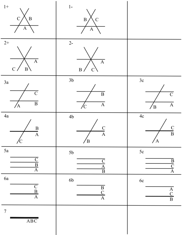
Recall that we have considered sets of (up to) three lines. If we consider triples of lines instead, cases (3) to (6) split up into three sub-cases, because they feature distinguishable lines. We then get 15 different configurations, which we name 1, 2, 3a, 3b, 3c, 4a, 4b, 4c, 5a, 5b, 5c, 6a, 6b, 6c and 7. While 5a, 5b and 5c correspond to case (5) above and therefore are comprised of infinitely many orbits, the remaining configurations are comprised of a single orbit.

The next split appears at the point when we consider qualitatively different configurations of triples of unoriented lines with respect to orientationpreserving affine bijections. An affine map f ( x, y ) = A ( x y ) + ( b x , b y ) is orientation-preserving if det ( A ) is positive. In the above arguments, we now have to consider oriented affine bases. Let us call an affine base ( p 1 , p 2 , p 3 ) positively (+) oriented, if the angle ∠ ( - - - → p 1 p 2 , - - - → p 1 p 3 ) is positive, otherwise, it is negatively ( -) oriented. Two given affine bases with the same orientation determine a unique orientation-preserving affine bijection transforming the first one into the second. Thus, the orientation of the affine base matters, and hence cases 1 and 2 above are split into two sub-cases each. For all the other cases, we have the freedom to choose the affine bases such that their orientations coincide. In the end, we get 17 different orbits of triples of oriented lines: 1+, 1-, 2+, 2-, 3a, 3b, 3c, 4a, 4b, 4c, 5a, 5b, 5c, 6a, 6b, 6c and 7. They are shown in Fig. 13

{ llllA } ↦→ LEFTleftA { llll+ , lllb+ , lllr+ } ↦→ LEFTleft+ { lrll , lbll } ↦→ LEFTleft -{ ffff , eses , fefe , fifi , ibib , fbii , fsei , ebis , iifb , eifs , iseb } ↦→ FRONTfront { bbbb } ↦→ BACKback { llbr } ↦→ LEFTback { llfl , lril , lsel } ↦→ LEFTfront { llrrP } ↦→ LEFTrightP { llrr+ } ↦→ LEFTright+ { llrf , llrl , llrr -, lfrr , lrrr , lere , lirl , lrri , lrrl } ↦→ LEFTright -{ rrrrA } ↦→ RIGHTrightA { rrrr+ , rbrr , rlrr } ↦→ RIGHTright+ { rrrr -, rrrl , rrrb } ↦→ RIGHTright -{ rrllP } ↦→ RIGHTleftP { rrll+ , rrlr , rrlf , rlll , rfll , rllr , rele , rlli , rilr } ↦→ RIGHTleft+ { rrll -} ↦→ RIGHTleft -{ rrbl } ↦→ RIGHTback { rrfr , rser , rlir } ↦→ RIGHTfront { ffbb , efbs , ifbi , iibf , iebe } ↦→ FRONTback { frrr , errs , irrl } ↦→ FRONTright { flll , ells , illr } ↦→ FRONTleft { blrr } ↦→ BACKright { brll } ↦→ BACKleft { bbff , bfii , beie , bsef , biif } ↦→ BACKfront { slsr } ↦→ SAMEleft { sese , sfsi , sisf } ↦→ SAMEfront { sbsb } ↦→ SAMEback { srsl } ↦→ SAMEright

GLYPH<15>

GLYPH<15>

GLYPH<15>

GLYPH<15>

/

/

Figure 11: Homomorphisms of weak representations from DRA fp to DRA opp

/

/

The structure of the orbits already gives us some insight into the nature of the dipole calculus. The fact that sub-case (1) corresponds to one orbit means that neither angles nor ratios of angles can be measured in the dipole calculus. By way of contrast, the presence of infinitely many orbits in sub-case (5) means that ratios of distances in a specific direction, not distances, can be measured in the dipole calculus. Indeed, in DRA fp , it is even possible to replicate a given distance arbitrarily many times, as indicated in Fig. 14.

That is, DRA fp can be used to generate a one-dimensional coordinate system. Note however that, due to the lack of well-defined angles, a twodimensional coordinate system cannot be constructed.

Note that Cristani's 2DSLA calculus [56], which can be used to reason about sets of lines, is too coarse for our purposes: cases (1) and (2) above cannot be distinguished in 2DSLA.

3.2 Computing the composition table with Condensed Semantics

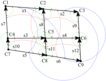
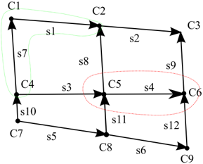
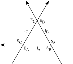
For the composition of (oriented) dipoles, we use the seventeen different configurations for triples of (unoriented) lines for the automorphism group of orientation-preserving affine bijections that have been identified in the previous section (Fig. 13). A qualitative composition configuration consists of a qualitative configuration for a triple of lines (the lines will serve as carrier lines for dipoles), carrying qualitative location information for the start and end points of three dipoles, as detailed in the sequel. While the notion of qualitative configuration composition is motivated by geometric notions, it is purely abstract and symbolic and does not refer explicitly to geometric objects. This ensures that it can be directly represented in a finite data structure.

Each of the three (abstract) lines l a A , l a B , l a C of a qualitative composition configuration carries two abstract segmentation points S X and E X ( X ∈ { A,B,C } ). P = { S A , S B , S C , E A , E B , E C } is the set of all abstract segmentation points.

In the geometric interpretation of these abstract entities (which will be defined precisely later on), the segmentation points lead to a segmentation of the lines. So, we introduce five abstract segments F , E , I , S , B (the letters are borrowed from the LR calculus). The set of abstract segments is denoted by S . It is ordered in the following sequence:

The geometric intuition behind this is shown in Fig. 15.

Having this segmentation of line configurations, we can introduce qualitative configurations for abstract dipoles by qualitatively locating their start and end points based on the above segmentation. In the case that two or more points fall onto the same segment, information on the relative location of points within that segment is needed; this is provided by an ordering relation denoted by < p .

By D , we denote the set S × S \ { ( S, S ) , ( E,E ) } (the exclusion of { ( S, S ) , ( E,E ) } is motivated by the fact that the start and end points of a dipole cannot coincide). By st ( dp ) and ed ( dp ), we denote the projections to the first and second components of each tuple, respectively. For convenience, we call the elements of the co-domains of st and ed abstract points.

Finally, we need information on the points of intersection of lines. Depending on orbit, there may be none, one, two or three points of intersection. Hence, we introduce sets ˆ S ( i ) with i ∈ { 1+ , 1 -, 2+ , 2 -, 3 a, 3 b, 3 c, 4 a, 4 b, 4 c, 5 a, 5 b, 5 c, 6 a, 6 b, 6 c, 7 } which give names to each abstract point of intersection. These sets are defined as:

where ˆ s XY denotes the point of intersection of abstract lines l a X and l a Y and ˆ s XYZ denotes the the point of intersection of the three abstract lines l a X , l a Y and l a Z .

In the geometric interpretation, we require segmentation points that coincide with points of intersection whenever possible. This coincidence is expressed via an assignment mapping , which is a partial mapping a : P ⇀ ˆ S ( i ) subject to the following properties:

• if a ( S X ) = ˆ s y , then y contains X ;
• if a ( E X ) = ˆ s y , then y contains X ;
• if both a ( S X ) and a ( E X ) are defined, then a ( S x ) = a ( E x ), for all X ∈ { A,B,C } ;
• the domain of a has to be maximal.

The first two conditions express that each abstract segmentation point is mapped to the correspondingly named abstract point of intersection. The third condition requires that the abstract segmentation points of a line cannot be mapped to the same abstract point of intersection. The last condition ensures that abstract segmentation points are mapped to abstract points of intersection whenever possible.

We now arrive at a formal definition:

Definition 29 (Qualitative Composition Configuration) . A qualitative composition configuration (qcc) consists of:

• An identifier i from the set { 1+ , 1 -, 2+ , 2 -, 3 a, 3 b, 3 b, 4 a, 4 b, 4 c, 5 a, 5 b, 5 c, 6 a, 6 b, 6 c, 7 } denoting one of the qualitatively different configurations of line triples as introduced in Section 3.1;
• An assignment mapping a : P ⇀ ˆ S ( i );
• A triple ( dp A , dp B , dp C ) of elements from D , where we call each such element an abstract dipole ;
• A relation < p on all points, i.e. the start and end points of the abstract dipoles, which is compatible with < .

Definition 30 (Abstract direction) . For any abstract dipole dp , we say that dir ( dp ) = + if and only if ed ( dp ) > p st ( dp ), otherwise dir ( dp ) = -.

glyph[negationslash]

3.2.1 Geometric Realization

In this section, we claim that each qcc has a realization, first of all, we need to define what such a realization is.

Definition 31 (Order on ray) . Given a ray l , for two points A and B , we say that A < r B , if B lies further in the positive direction than A .

We construct a map on each ray that reflects the abstract segments shown in Fig. 15 to provide a link between a qcc and a compatible line scenario.

Definition 32 (Segmentation map) . Given a ray r and two points ˜ S and ˜ E on it, the segmentation map seg : r -→ { ˜ F, ˜ E, ˜ I, ˜ S, ˜ B } is defined as:

for any point on x on r .

When it is clear that we are talking about segments on an actual ray, we often omit the ˜.

Definition 33 (Geometric Realization) . For any qcc Q a geometric realization R ( Q ) consists of a triple of dipoles ( d A , d B , d C ) in R 2 , three carrier rays l A , l B , l C of the dipoles, and two points ˜ S X and ˜ E X on l X for each X ∈ { A,B,C } , such that:

• ( l A , l B , l C ) (more precisely, the corresponding triple of unoriented lines) belongs to the configuration denoted by the identifier i of Q ;
• the angle between l a and the other two rays must lie in the interval ( π, 2 · π ];
• for any x, y ∈ ˜ P , if a ( p ( x )) and a ( p ( y )) are both defined and equal, then x = y (where p : ˜ P = { ˜ S A , ˜ S B , ˜ S C , ˜ E A , ˜ E B , ˜ E C } → P be the obvious bijection);
• for all X , st ( dp X ) = seg ( st ( d X )) and ed ( dp X ) = seg ( ed ( d X ));
• for all points x and y on l X , if seg ( x ) < seg ( y ), then x < r y ;
• if l X = l Y , the order < p must be preserved for points st ( d X ), ed ( d X ), st ( d Y ), ed ( d Y ), in such a way that: if st ( dp X ) < p st ( dp Y ), then st ( d Y ) < r st ( d X ) and in the same manner between all other points.

must hold.

Proposition 34. Given three dipoles in R 2 , there is a qcc Q and a geometric realization of R ( Q ) which uses these three dipoles.

Proof. For this proof, we construct a qcc from a scenario of three dipoles in R 2 . Given three dipoles d A , d B , d C in R 2 , we determine their carrier rays l A , l B , l C in such a way that the angles between l A and l B as well as l A and l C lie in the interval ( π, 2 · π ]. We determine the identifier of the configuration in which the the scenario lies. We determine the points of intersection of the rays and identify them with ˆ s XY in ˆ S ( i ). For all points X in P , for which a is undefined, the points ˆ X are placed in such a way, that S X < r E X (which is equivalent to S X < E X ). We identify st ( dp X ) and ed ( dp X ) according to the segmentation map on these rays. If two carrier rays coincide, we define the order < p w.r.t. < r , otherwise it is arbitrary. This clearly gives a qcc .

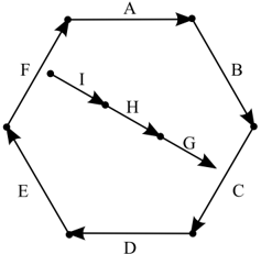
An example of this construction is given in Fig. 16. On the left-hand-side

of Fig. 16, there is a scenario with three dipoles, lying somewhere in R 2 . On the right hand side, rays and points of intersection are added. Comparison with orbits and placement of lines determine the identifier 3 b for this scenario. The map a can be defined as

where the assignment is only free for E A and E B . E A and E B are lying at the start point of dipole d A and at the end point of dipole d B . In this way, we get:

and instead of

In this case the assignment of < p is arbitrary.

This construction gives us the desired qcc and a realization of it.

3.3 Primitive Classifiers

The last and most crucial point is the computation of DRA relations between three dipoles. We can decompose this task into subtasks, since each DRA f relation comprises four LR relations between a dipole and point; these are obtained from a qualitative composition configuration using so-called primitive classifiers . The basic classifiers apply the primitive classifiers to the abstract dipoles in each qualitative composition configuration in an adequate manner. For DRA fp relations an extension of the basic classifiers is used in cases where the qualitative angle between several dipoles has to be determined. Finally, the resulting data is collected in a (composition) table.

Definition 35 (Primitive Qualitative Composition Configuration) . A primitive qualitative composition configuration (pqcc) is a sub-configuration of a qualitative composition configuration (see Def. 29) containing two abstract dipoles (where for the second one, only the start or end point is used for classification). All other data are the same as in Def. 29.

Notation 36. To simplify the explanation of large classifiers, we shall write:

If it is clear which function we are defining, we even omit the ' f ( x ) ='.

Given a primitive qualitative composition configuration Q , primitive classifiers map the qualitative locations of a dipole dp 1 and a point pt (which is the start or end point of another dipole dp 2 ) to a letter indicating the LR relation between the dipole and point. We say that the dipole has positive pos orientation if dir ( dp ) = +, otherwise the orientation is negative neg .

We need three different types of primitive classifiers for our algorithm.

Given two arbitrary dipoles dp 1 and dp 2 , we construct a primitive classifier for a pqcc with intersecting carrier rays in its realization. The classifier itself only works on dp 1 and pt , where pt is either the start or end point of dp 2 . A

realization of this pqcc is given in Fig. 17 for the reader's convenience, the actual dipoles are omitted from the figure, since they can be placed arbitrarily.

To realize the dipole, this classifier takes dipole dp 1 and the start or end point of dp 2 called pt as well as information on whether dp 1 is pointing in the same direction as the ray ( pos ) or against it ( neg ) for both dipoles. The classifier returns an LR -relation determining the relation between dp 1 and pt .

In this case, the classifier cli x,y ( dp 1 , pt ) is given by:

The subscripts on the classifier denote the point of intersection of the two lines. For the case shown in Fig. 17, we have x = y = S . We see that the table for neg is exactly the complement of pos . This primitive classifier assumes that, in the geometric realization, the second dipole (containing point pt ) points to the right w.r.t. dipole d . If the second dipole points to the left in the realization, it is sufficient to apply an operation that interchanges L with R on this classifier, in order to obtain the correct results. We will call this operation com . This is the only primitive classifier needed for intersecting lines.

Secondly, we give a primitive classifier cls ( dp 1 , pt ) for two lines that coincide, see Fig. 18.

neg -→                                                                                                                                                                pt = B -→                          st ( dp 1 ) > B ∧ ed ( dp 1 ) > B -→ F st ( dp 1 ) > B ∧ ed ( dp 1 ) = B -→    ed ( dp 1 )
p pt -→ F st ( dp 1 ) = B ∧ ed ( dp 1 ) = B -→            st ( dp 1 )
p pt ∧ ed ( dp 1 )
p pt ∧ ed ( dp 1 ) = p pt -→ E st ( dp 1 ) >p pt ∧ ed ( dp 1 ) >p pt -→ F pt = S -→            st ( dp 1 ) > S ∧ ed ( dp 1 ) > S -→ F st ( dp 1 ) > S ∧ ed ( dp 1 ) = S -→ E st ( dp 1 ) > S ∧ ed ( dp 1 ) < S -→ I st ( dp 1 ) = S ∧ ed ( dp 1 ) < S -→ S st ( dp 1 ) < S ∧ ed ( dp 1 ) < S -→ B pt = I -→                                              st ( dp 1 ) > I ∧ ed ( dp 1 ) > I -→ F st ( dp 1 ) > I ∧ ed ( dp 1 ) = I -→    ed ( dp 1 ) >p pt -→ F ed ( dp 1 ) = p pt -→ E ed ( dp 1 )
I ∧ ed ( dp 1 ) < I -→ I st ( dp 1 ) = I ∧ ed ( dp 1 ) = I -→            st ( dp 1 ) >p pt ∧ ed ( dp 1 ) >p pt -→ F st ( dp 1 ) >p pt ∧ ed ( dp 1 ) = p pt -→ E st ( dp 1 ) >p pt ∧ ed ( dp 1 )
p pt -→ I st ( dp 1 ) = p pt -→ S st ( dp 1 )
E ∧ ed ( dp 1 ) > E -→ F st ( dp 1 ) > E ∧ ed ( dp 1 ) = E -→ E st ( dp 1 ) > E ∧ ed ( dp 1 ) < E -→ I st ( dp 1 ) = E ∧ ed ( dp 1 ) < E -→ S st ( dp 1 ) < E ∧ ed ( dp 1 ) < E -→ B pt = F -→                          st ( dp 1 ) = F ∧ ed ( dp 1 ) = F -→            st ( dp 1 ) >p pt ∧ ed ( dp 1 ) >p pt -→ F st ( dp 1 ) >p pt ∧ ed ( dp 1 ) = p pt -→ E st ( dp 1 ) >p pt ∧ ed ( dp 1 )
p pt -→ I st ( dp 1 ) = p pt -→ S st ( dp 1 )

This classifier looks a little cumbersome, but we decided to use it in this way, so that all impossible cases w.r.t. the ordering of the line are excluded. This gives better error handling capabilities in an implementation of it, since impossible cases can be detected. A more compressed version is possible, but it cannot detect impossible cases anymore. All cases that are not listed in the above classifier are cases where the ordering > p is not compatible with the segmentation, and so they are impossible. This is the only classifier for coinciding lines.

The third classifier is for parallel lines, i.e. a configuration like that in Fig. 19. Let the lower line be the line the dipole lies on. The information about the line on which the dipole lies is handled by a basic classifier which uses this primitive classifier and exchanges L and R appropriately. Fortunately this

classifier clpar ( dp 1 , pt ) is simple:

This is the only classifier for parallel lines.

This is a complete list of the basic classifiers that are needed.

3.4 Basic Classifiers

Based on the primitive classifiers introduced in Sect. 3.3, we construct the basic classifiers to determine the DRA relations in scenarios. For DRA f , we always need exactly four primitive classifiers to determine the relation. For DRA fp , in some cases we need an additional fifth classifier to determine the qualitative angle. We will first focus on the DRA f case. Given a qcc, we apply four basic classifiers three times: namely (1) to the first and second abstract dipole, (2) to the second and third and (3) to the first and third. Thus, we obtain an entry in the composition table. Consider a qcc with i = 1+ and a ( S A ) = ˆ s AB , a ( S B ) = ˆ s AB and a ( s C ) = ˆ S AC . Such a configuration has a realization as in Fig. 20. The dipole d X lies on the ray l X for X ∈ { A,B,C } . We now apply

primitive classifiers to this scenario in the way defined in Section 2.1. Hence, we get the basic classifier for such a configuration:

and we obtain the relation between dp A and dp B : glyph[rho1] ( R ( dp A , st B ) , R ( dp A , ed B ) , R ( dp B , st A ) , R ( dp B , ed A )). The relations between d B and d C as well as between dp A and dp C are derived analogously. The basic classifiers depend on the configuration in which the qcc realization lies and on the angle between the rays in the realization. They are constructed for an angle between the rays in the interval ( π, 2 · π ]. If the angle is in the interval (0 , π ], the LR relation between any line on the first ray and a point on the second just swaps. We capture this by introducing the operation com which is applied in this case. With it, we can limit the number of necessary primitive classifiers. The construction of the other basic classifiers is done analogously.

3.5 Extended Basic Classifiers for DRA fp

For DRA fp , basically the same classifiers as described for DRA f in Section 3.4 are used. We simply extend them for the relations rrrr, rrll, llll and llrr to classify the information about qualitative angles. For this purpose, we have to have a look at the angles between dipoles in the realization of a given qcc. The qualitative angle between two dipoles d A and d B is called positive + (negative -) if the angle from the carrier ray of d A called l A to the carrier ray of d B called l B lies in the interval (0 , π ) (( π, 2 · π )). We give an example of this. Consider the configuration of a DRA scenario in Fig. 21 on the left hand side. On the right-

hand side of Fig. 21, the carrier rays are introduced and we can see that the angle clearly lies in the interval (0 , π ) and hence the qualitative angle is positive. The definitions of parallel P and anti-parallel A are straightforward. The set a -1 ( ˆ S xy ) always contains exactly two elements, if ˆ S xy ∈ ˆ S ( i ). To continue, we need functions proj x : P ( P ) -→ P ( P ) defined as

which form the set of all elements with index ( idx ) x. P denotes powerset formation. By the definition of a and the sets ˆ S ( i ), these sets are always singletons, if proj x ◦ a -1 is applied to an intersection point and if a -1 contains an element with index x , otherwise the set is empty. We shall write a -1 x for proj x ◦ a -1 .

We observed that the qualitative angles between two dipoles can be classified very easily once the DRA f relations between the dipoles d A and d B are known. All we need to do is to find out if the ray l B intersects l A in front of or behind d A . In the language of qcc and abstract dipoles dp A and dp B , we can say that, if a -1 A ( ˆ S AB ) > ed ( dp A ) for dir ( dp A ) = +, or if a -1 A ( ˆ S AB ) < ed ( dp A ), if dir ( dp A ) = -, then the abstract point of intersection lies 'in front of dp A ' and, if st ( dp A ) > a -1 A ( ˆ S AB ) for dir ( dp A ) = + or a -1 A ( ˆ S AB ) > st ( dp A ) for dir ( dp A ) = -, the abstract point of intersection lies 'behind dp A '.

Proposition 37. In a realization R ( Q ) of a qcc Q , the carrier rays of any two dipoles d 1 and d 2 intersect in front of d 1 if and only if, in Q the property

is fulfilled.

Proof. This is immediate by inspection of the property and respective scenarios.

Proposition 38. In a realization R ( Q ) of a qcc Q , the carrier rays of any two dipoles d 1 and d 2 intersect behind d 1 if and only if, in Q the property

is

Proof. This is immediate by inspection of the property and respective scenarios.

The complete extension for the Basic Classifiers is given as:

Constructing the classifiers for qccs based on configurations with parallel lines is easy, depending on the DRA f -relations, the dipoles can either be parallel or anti-parallel in such cases, but never both at the same time.

Lemma 39. Given two intersecting lines, the LR -relations between a dipole on a first line and a point on the second line are stable under the movement of the point along the line, unless it moves through the point of intersection of the two lines.

Proof. By the definition of LR -relations, the point can be in one of three different relative positions to the carrier ray of the dipole. The point can lie on either side of the point of intersection, yielding the relation L or R , or on the point of intersection itself, yielding exactly one relation on the line.

Lemma 40. Given a dipole and a point lying on its carrier line, the LR -relations between the dipole and point are stable under the movement of the point along the line, unless it is moved over the start or end point of the dipole.

Proof. Inspect the definition of LR -relations on a line.

Lemma 41. For dipoles lying on intersecting rays, the DRA relations are stable under the movement of the start and end points of the dipoles along the rays, as long as the segments for the start and end points and the directions of the dipoles do not change.

Proof. We observe that the segmentation is a stronger property than the one used in Lemma 39. For DRA f relations it suffices to apply Lemma 39 four times. For DRA fp relations, we also need to take the intersection property of Prop. 46 into account.

Lemma 42. For dipoles on the same line, the DRA -relations are stable under the movement of the start and end points of the dipoles along the rays, so long as the relation < r does not change.

• Lemma 43. 1. Transforming a given realization of a qcc along an orientation-preserving affine transformation preserves the segmentation map.
• If two dipoles are on the same line, affine transformations also preserve < r .

Proof. 1) According to Prop. 28, any orientation-preserving affine transformation preserves the LR relations.

2) This follows from the preservation of length ratios by affine transformations, i.e. the length ratios between the start and end points of the dipoles and points S and E on the ray.

Lemma 44. Given a qcc, any two geometric realizations exhibit the same DRA -relations among their dipoles.

Proof. Let two geometric realizations R 1 , R 2 of a qcc Q be given. Since the line triples of R 1 and R 2 belong to the same orbit, there is an orientationpreserving affine bijection f transforming the line triple of R into that of R ′ . In case of configurations 5a, 5b and 5c, we assume that all distance ratios are adjusted to 1 in order to reach the same orbit. Note that this adjustment, although not an affine transformation, does not affect the relations between dipoles.

Since f maps R 1 's line triple to R 2 's line triple, it also maps the corresponding points of intersection to each other. For orbits 1+ and 1 -, all segmentation points are points of intersection. Hence, f does not change the segments given by r ( x ) in which the start and end points of the dipoles lie. For the rest of the argument, apply Lemma 41.

For cases 2+ and 2 -, we just have a single point of intersection, but the relative directions of the rays are restricted by the definition of a realization and so is the location of all segmentation points w.r.t. the intersection point, as are the locations of the start and end points of the dipoles w.r.t. the segmentation points. For the rest of the argument, apply Lemma 41.

In cases 3 a , 3 b and 3 c , we have two intersection points and two segmentation points that are not points of intersection but, as before, the directions of the rays and the locations of all segmentation points are restricted and hence the locations of the start and end points of the dipoles, and again, we can apply Lemma 41.

In cases 4 a , 4 b and 4 c , we have one point of intersection and 3 segmentation points that are not points of intersection. First, we can argue to restrict the location and direction. In the end, we can apply Lemma 42 and Lemma 41.

In cases 5 a , 5 b and 5 c , we only have segmentation points that are not points of intersection, but all rays have the same directions and the relative orientations of segmentation points on the line are restricted. Hence, the directions of the dipoles do not change during the mapping and the relative direction between

dipoles is all that is necessary to determine their DRA -relations in the case of parallel dipoles.

The proof of cases 6 a , 6 b and 6 c is similar to cases 4 and 5, with the argument based on Lemma 42 for dipoles on the same line, and the arguments of cases 5 for parallel lines.

For case 7, we need to apply Lemma 42.

For additional arguments for DRA fp -relations, please refer to the proof of Prop. 46.

Theorem 45 (Correctness of the Construction) . Given a qcc Q and an arbitrary geometric realization R ( Q ) of it, the DRA f relation in R ( Q ) is the same as that computed by the basic classifiers on Q .

Proof. According to Lemma 44, we can focus on one geometric realization per qcc.

For this proof, we need to inspect once more the construction of the basic classifiers above the primitive classifiers. The actual values of a , dir and the start and end points of the abstract dipoles as well as the order < p are not directly used by basic classifiers 19 . They are passed through to primitive classifiers. The only information that is directly used in basic classifiers is the identifier i of the configuration.

We divide this proof in two steps. In the first step, we show that the primitive classifiers are correct and, in the second step, we do the same for basic classifiers. We will show a proof for the classifier cli S,S ( dp 1 , pt ) and a pqcc with dir dp 1 = +, dp 1 = ( I, I ) and pt = I . A realization of this configuration is shown in Fig. 22 and we can easily see that d 1 R pt has to be true. By observing cli S,S ( dp 1 , pt ),

we see that we are in the case pos and that pt > S and so the primitive classifier also yields dp 1 R pt as expected. All other proofs for pqccs are done in an analogous way by inspection of the relations yielded by the primitive classifiers and their realizations. With primitive classifiers working correctly, we need to focus on the basic classifiers. Here, we will show this for the case i = 1+, all other cases are handled in an analogous fashion. First we take any realization of i = 1+ and add directions to the lines as described in the section about

19 With the exception of the extended classifiers, but we will discuss these later

geometric realizations of qccs. For example, the one depicted in Fig. 23. In the

next step, this realization is decomposed according to the definition of DRA f -relations and the basic classifiers shown in Fig. 24. The various parts of the

decomposed line configuration need to be matched with the realization of the primitive classifier, here the realization of Fig. 17. In our case, the classifier matches directly with the orientations from l A to l B , l B to l C and l A to l C . In the other cases, the angle between the lines may be inverted. Then, we need to swap R and L which is done by the operation com . Furthermore, we see that the lines l C and l B both intersect in segment E , whereas l A and l B intersect both in S . The intersection for l A and l C is E for l A and S for l C , we need to parameterize the respective primitive classifiers with that information. But in the end, our arguments yield exactly the basic classifier shown in Section 3.4. The arguments for the other 16 basic classifiers are analogous.

Proposition 46. Given any qcc Q and its geometric realization R ( Q ) , the extended basic classifiers determine the same DRA fp relation as in the realization.

Proof. We assume that the DRA f relation is determined correctly. All we need to consider here are the 'extended' relations.

We will give the proof for rrrr-, the proof for the other cases is analogous. Consider two dipoles d A and d B in an rrrr configuration on the rays l A and

l B . There are two classes of qualitatively distinguishable configurations for ( d A rrrr d B ):

Wecan see that l B intersects l A either in front of or behind d A . If the intersection point lies in front of d A , we are in a situation like

where S is the intersection point. We can further see that the angle from l A to l B lies clearly in the interval ( π, 2 · π ). Furthermore, l B can be rotated in the whole interval ( π, 2 · π ) without changing the DRA f relation. Using this, we obtain the DRA fp -relation rrrr- between d A and d B if the point of intersection S lies in front of d A . For any qcc belonging to such a scenario, the rest of the proof follows from Prop. 37 and Prop. 38 as well as the inspection of the extended classifiers:

But these also yield ( dp A rrrrdp B ). By the same arguments, we show that ( d A rrrr+ d B ) if the point of intersection of l A and l B lies behind d A . The proof for all other cases is analogous.

Corollary 47. The 72 relations in Fig. 3 are those out of the 2401 formal combinations of four LR letters that are geometrically possible.

Proof. By an exhaustive inspection of the primitive classifiers which occur in the basic classifiers for all pqccs. For the decomposition, we refer to the proof of Thm. 45.

Theorem 48. Given a qcc Q and an arbitrary geometric realization R ( Q ) of it, the DRA fp relation in R ( Q ) is the same as that computed by the basic classifiers on Q .

Proof. Follows from Thm. 45 and Prop. 46.

3.6 Implementation of the Classification Procedure

Qualitative composition configurations can be naturally represented as a finite datatype. The classifiers are implemented as simple programs (mainly case distinctions) that operate on qccs in the sense of Def. 29. The classifiers are chosen with respect to the identifier i and the assignment mapping a of the qcc . In our particular implementation, we exploited some symmetries to limit the number of classifiers that we had to implement.

With the condensed semantics, we are able to compute the composition tables of the DRA calculi in an efficient way. In fact we have implemented the computation of composition tables for both DRA f and DRA fp as Haskell programs, making use of Haskell's parallelism extensions. The Haskell implementations of the basic classifiers for DRA f and DRA fp are written in such a way that they share a library of primitive classifiers. In these programs, we further generate all qccs in an optimized way, i.e. we only generate the order < p if it is needed, and classify them with our basic classifiers. In the end, we compose our results into composition tables. For the case where three lines are collinear, we simply decided to enumerate all possible locations of points in a certain interval for reasons of simplicity and this did not increase the overall runtime too much.

The computation of the composition table for DRA f takes less than one minute on a Notebook with an Intel Core 2 T7200 with 1 . 5 Gbyte of RAM, and the computation of the composition table for DRA fp takes less than two minutes on the same computer. This is a great advancement compared to the enumeration of scenarios on a grid, which took several weeks to compute only an approximation to the composition table.

3.7 Properties of the Composition

We have investigated several properties of the composition tables for DRA f and DRA fp . For both tables the properties

hold with R , R 1 , R 2 , R 3 being any base-relation and id the identical relation. These properties can be automatically tested by the GQR and SparQ qualitative reasoners. The other properties for a non-associative algebra follow trivially. Furthermore, we have tested the associativity of the composition. For DRA f , we have 373248 triples of relations to consider of which 71424 are not associative. So the composition of 19 . 14% of all possible triples of relations is not

associative 20

glyph[negationslash]

, e.g. (rrrl; rrrl); llrl = rrrl; (rrrl; llrl) .

For DRA fp all 512000 triples of base-relations are associative w.r.t. composition. With this result, we obtain that DRA fp is a relation algebra in a strict sense.

3.8 DRA f composition is weak

The failure of DRA f to be associative may imply that its composition is also weak. We will investigate this in this section. First, recall the definition of strong composition. Furthermore, the composition of OPRA 1 is known to be weak [49], but by Ex. 19 and Prop. 20, then DRA f also has a weak composition.

Definition 49. A Qualitative Composition is called strong if, for any arbitrary pair of objects A , C in the domain in relation Ar ac C , there is for every entry in the composition table that contains Ar ac C on the right hand side, an object B such that Ar ab B and Br bc C reconstruct this entry.

We will show now that the defining property of strong composition (see Sect. 2.3) is violated for DRA f .

Proposition 50. The composition of DRA f is weak.

Proof. Consider the DRA f composition A BFII B ; B LLLB C ↦→ A LLLL C . We show that there are dipoles A and B such that there is no dipole B which reflects the composition. Consider dipoles A and B as shown in Fig. 25. We observe that they are in the DRA fp relation LLLL- with the dipole

C pointing towards the line dipole A lies on. Because of A BFII B , dipole B has to lie on the same line as A . But, since C is a straight line and lines A and B lie in front of C , the endpoint of B cannot lie behind C .

As expected, the composition of DRA f turns out to be weak. Let us have a closer look at the composition of DRA fp in the next section.

20 In the master thesis of one of our students, a detailed analysis of a specific non-associative dipole configuration is presented [57]

3.9 Strong Composition

We are now going to prove that DRA fp has a strong composition. The following lemma will be crucial; note that it does not hold for DRA f .

Lemma 51. Let R be a DRA fp base relation. For DRA fp base relations R not involving parallelism or anti-parallelism, betweenness and equality among { s A , e A , S A,B } 21 for given dipoles ARB are independent of the choice of A and B , hence uniquely determined by R alone.

glyph[negationslash]

Proof. Let R = r 1 r 2 r 3 r 4 r 5 , where r 5 ∈ { + , -} even if r 5 this is omitted in the standard notation. Note that the assumption r 5 ∈ { + , -} implies that S A,B is defined. If r 3 ∈ { b, s, i, e, f } , e A = s A = S A,B , hence there is no betweenness. Analogously, s A = e A = S A,B if r 4 ∈ { b, s, i, e, f } . The remaining possibilities for r 3 r 4 r 5 are:

glyph[negationslash]

1. ll+, rr-: in these cases, e A is between s A and S A,B ;
2. ll-, rr+: in these cases, s A is between e A and S A,B ;
3. rl-, lr+: in these cases, S A,B is between s A and e A .

Note that cases 1 and 2 cannot be distinguished in DRA f .

Corollary 52. Let R be a DRA fp base relation not involving parallelism or anti-parallelism. Let ARB and A ′ RB ′ . Then, the map { s A ↦→ s A ′ ; e A ↦→ e A ′ ; S A,B ↦→ S A ′ ,B ′ } preserves betweenness and equality.

Lemma 53. Let R be a DRA fp base relation not involving parallelism or antiparallelism. Given dipoles ARC and A ′ RC ′ and points p A , p A ′ , p C and p C ′

21 Please remember that s A = st ( dp A ) and e A = ed ( dp A ).

on the lines carrying A , A ′ , C and C ′ respectively, if the maps { s A ↦→ s A ′ , e A ↦→ e A ′ , S A,C ↦→ S A ′ ,C ′ , p A ↦→ p A ′ } and { s C ↦→ s C ′ , e C ↦→ e C ′ , S A,C ↦→ S A ′ ,C ′ , p C ↦→ p C ′ } preserve betweenness and equality, then the angles ∠ ( - - - - - → S A,C p A , - - - - - → S A,C p C ) and ∠ ( - - - - - → S A,C p A , - - - - - → S A,C p C ) have the same sign.

Proof. Since ARC and A ′ RC ′ , the angles ∠ ( -- - → s A e A , -- - → s C e C ) and ∠ ( -- - - → s A ′ e A ′ , -- - - → s C ′ e C ′ ) have the same sign. By the assumption of the preservation of betweenness and equality, this carries over to angles ∠ ( - - - - - → S A,C p A , - - - - - → S A,C p C ) and ∠ ( - - - - - → S A,C p A , - - - - - → S A,C p C ).

Theorem 54. Composition in DRA fp is strong.

Proof. Let r ac ∈ r ab ◦ r bc be an entry in the composition table, with r ac , r ab and r bc base relations. Given dipoles A and C with Ar ac C , we need to show the existence of a dipole B with Ar ab B and Br bc C .

Since r ac ∈ r ab ◦ r bc , we know that there are dipoles A ′ , B ′ and C ′ with A ′ r ab B ′ , B ′ r bc C ′ and A ′ r ac C ′ . Given dipoles X and Y , let S X,Y denote the point of intersection of the lines carrying X and Y ; it is only defined if X and Y are not parallel. Consider now the three lines carrying A ′ , B ′ and C ′ , respectively. According to the results of Section 3.1, for the configuration of these three lines, there are fifteen qualitatively different cases 1, 2, 3a, 3b, 3c, 4a, 4b, 4c, 5a, 5b, 5c, 6a, 6b, 6c and 7:

1. The three points of intersection S A ′ ,B ′ , S B ′ ,C ′ and S A ′ ,C ′ exist and are different. Since Ar ac C and A ′ r ac C ′ , by Corollary 51, the point sets { s A , e A , S A,C } and { s A ′ , e A ′ , S A ′ ,C ′ } are ordered in corresponding ways on their lines. Hence, it is possible to choose S A,B in such a way that the point sets { s A , e A , S A,C , S A,B } and { s A ′ , e A ′ , S A ′ ,C ′ , S A ′ ,B ′ } are ordered in corresponding ways on their lines. In a similar way (interchanging A and C ), S B,C can be chosen.

Since both { S A,B , S A,C , S B,C } and { S A ′ ,B ′ , S A ′ ,C ′ , S B ′ ,C ′ } are affine bases, there is a unique affine bijection h : R 2 -→ R 2 with h ( S A ′ ,B ′ ) = S A,B , h ( S A ′ ,C ′ ) = S A,C and h ( S B ′ ,C ′ ) = S B,C . By Lemma 53, h preserves orientation, and thus by Thm. 28 also the DRA fp relations. Hence, by choosing B = h ( B ′ ), we get h ( A ′ ) r ab B and Br bc h ( C ′ ). Since the sets

• { s A , e A , S A,C , S A,B } and { h ( s A ′ ) , h ( e A ′ ) , S A,C , S A,B } are on the same line and have corresponding qualitative (betweenness) relations, and the same holds for the sets { s C , e C , S A,C , S B,C } and { h ( s C ′ ) , h ( e C ′ ) , S A,C , S B,C } , we also have Ar ab B and Br bc C (even though h ( A ′ ) = A and h ( C ′ ) = C do not necessarily hold).

glyph[negationslash]

1. The three intersection points S A ′ ,B ′ , S B ′ ,C ′ and S A ′ ,C ′ exist and coincide, i.e. S A ′ ,B ′ = S B ′ ,C ′ = S A ′ ,C ′ =: S ′ . Let S = S A,C . Let x A be s A and x A ′ be s A ′ if s A = S (and therefore s A ′ = S ′ ), otherwise, let x A be e A and x A ′ be e A ′ . x C and x C ′ are chosen in a similar way. Since both { S, x A , x C } and { S ′ , x A ′ , x C ′ } are affine bases, there is a unique affine bijection h : R 2 -→ R 2 with h ( S ′ ) = S , h ( x A ′ ) = x A and h ( x C ′ ) = x C . The rest of the argument is similar to case (1).

glyph[negationslash]

1. (Two lines are parallel and intersect with the third one.) In the sequel, we will just specify how two affine bases are chosen; the rest of the argument (as well as the choice of points on the unprimed side in such a way that qualitative relations are preserved) is then similar to the previous cases. Subcases (3a), (3b): The lines carrying A and C intersect. Choose x A and x A ′ as in case (2), and chose an appropriate point S B,C . Then use the affine bases { x A , S A,C , S B,C } and { x A ′ , S A ′ ,C ′ , S B ′ ,C ′ } . Subcase (3c): The lines carrying A and C are parallel. Choose appropriate points S A,B and S B,C and use the affine bases { s A , S A,B , S B,C } and { s A ′ , S A ′ ,B ′ , S B ′ ,C ′ } .

glyph[negationslash]

1. (Two lines are identical and intersect with the third one.) Subcases (4a) and (4b): The lines carrying A and C intersect. Choose x A , x A ′ , x C and x C ′ as in case (2) and use the affine bases { S A,C , x A , x C } and { S A ′ ,C ′ , x A ′ , x C ′ } . Subcase (4c): The lines carrying A and C are identical. This means that S A ′ ,B ′ = S A ′ ,C ′ =: S ′ . Choose an appropriate point S and x A , x A ′ as in case (2). Moreover, in a similar way, choose x B ′ = S ′ , and then some corresponding x B being in the same LR -relation to A as x B ′ has to A ′ . Then use the affine bases { S, x A , x B } and { S, x A ′ , x B ′ } .
2. (All three lines are distinct and parallel.) Subcases (5a), (5b) and (5c) can all be treated in the same way: Use the affine bases { s A , e A , s C } and { s A ′ , e A ′ , s C ′ } . Note that the distance ratio does not matter here.
3. (Two lines are identical and are parallel to the third one.) Subcases (6a) and (6b): The lines carrying A and C are parallel. Proceed as in case (5). Subcase (6c): The lines carrying A and C are identical. Choose some s B in the same LR -relation to A as s B ′ is to A ′ . Then use the affine bases { s A , e A , s B } and { s A ′ , e A ′ , s B ′ } .
4. (All three lines are identical.) For this case, the result follows from the fact that Allen's interval algebra has strong composition (refer to [26]).

Proof.

opp is strong as well. By Example 19 and Prop. 20.

4 Constraint Reasoning with the Dipole Calculus

4.1 Consistency

We now consider the question of whether algebraic closure decides consistency. We call the set of constraints between all dipoles at hand a constraint network . If no constraint between two dipoles is given, we agree that they are in the universal relation. By scenario , we denote a constraint network in which all constraints are base-relations 22 . We construct constraint-networks which are geometrically unrealizable but still algebraically closed. We do this by constructing constraint networks that are consistent and algebraically closed, and then we will change a relation in them in such a way that they remain algebraically closed but become inconsistent. We follow the approach of [58] in using a simple geometric shape for which scenarios exist, where algebraic closure fails to decide consistency. In our case, the basic shape is a convex hexagon, similar to a screw head.

Consider a convex hexagon consisting of the dipoles A , B , C , D , E and F . Such an object is described as

( A errs B )( B errs C )( C errs D )( D errs E )( E errs F )( F errs A )

where the components r of the relations ensure convexity, since they enforce an angle between 0 and π between the respective first and second dipole, i.e., the endpoint of consecutive dipoles always lies to the right of the preceding dipole. Such an object is given in Fig. 26 To this scenario we add a seventh dipole G with the relations

( G rrll A )( G lrll F )( G llrr D )( G rlrr C )

We have the overall constraint network:

( A errs B )( B errs C )( C errs D )( D errs E )( E errs F )( F errs A ) ( G rrll A )( G lrll F )( G llrr D )( G rlrr C )

Because of the relations ( G lrll F ) and ( G rlrr C ), line l G intersects line l F as well as line l C . Because of the first two components of the relations, dipoles F and C are oriented into qualitatively antipodal directions. This network is consistent and is of course algebraically closed.

22 In this case, a base-relation between every pair of distinct dipoles has to be provided

To construct an inconsistent network, we change the relation ( G rlrr C ) to ( G rlll C ) and obtain the constraint network:

( A errs B )( B errs C )( C errs D )( D errs E )( E errs F )( F errs A ) ( G rrll A )( G lrll F )( G llrr D )( G rlll C )

The relations ( G rlll C ) and ( G lrll F ) enforce that G must lie in between F and C as shown in Fig. 27. In this case, the all convex hexagons A , B , C , D ,

E , F have the endpoints of consecutive dipoles lying to the left of the preceding one, they are of the form:

( A ells B )( B ells C )( C ells D )( D ells E )( E ells F )( F ells A )

which is a contradiction of the required form of hexagon in the scenario. In fact there is no affine transformation which preserves the relative orientations between dipoles A , B , C , D , E , F , and maps a hexagon of Fig. 26 to any that can be constructed along dipoles C and F in Fig. 27 in such a way that the edges C and F of both hexagons coincide. Still algebraic closure with DRA f

yields the refinement:

( F lllr G )( E (flll , llll , rfll , rlll , rrll) G )( D errs E )( D rrll G ) ( D (rbrr , rllr , rlrr , rrrr) F )( C llrl G )( C (lrrl , rllr) F )( E errs F ) ( C (rllr , rrfr , rrlr , rrrr) E )( C errs D )( B (llrr , rrrr) G ) ( B (blrr , llll , llrf , llrl , llrr , rfll , rlll , rlrr, rrbl , rrll , rrrl , rrrr) E ) ( B (rbrr , rlrr , rrfr , rrlr , rrrr) D )( B errs C )( A llrr G )( A rser F ) ( A (frrr , lrrr , rrrb , rrrl , rrrr) E)(A (rllr , rlrr , rrrr) C ) ( A (lfrr , llbr , llll , lllr , llrr , lrll , lrrr , rrlf , rrll , rrlr , rrrr) D ) ( B (frrr , lrrl , lrrr , rrrr) F )( A errs B )

A scenario,

( F lllr G )( E flll G )( E errs F )( D rrll G )( D rrrr F )( D errs E ) ( C llrl G )( C rllr F )( C rrlr E )( C errs D )( B llrr G )( B lrrl F ) ( B llrl E )( B rlrr D )( B errs C )( A llrr G )( A rser F )( A rrrr E ) ( A lrrr D )( A rllr C )( A errs B )

can be derived from this algebraically closed network. It is still deemed algebraically closed, even though it is not consistent with the same argument given above. Hence algebraic closure does not decide consistency for DRA f -scenarios. On the other hand, algebraic closure with DRA fp detects all possible extensions of this network to that calculus as being inconsistent. Extending the consistent case with the relation ( G rlrr C ) yields three possible extensions for DRA fp scenarios, of which all are consistent. In fact, we get the three following consistent refinements.

DRA f -relation	refinement1	refinement2	refinement3
( G rrll A )	( G rrll- A )	( G rrll- A )	( G rrll- A )
( G llrr D )	( G llrr- D )	( G llrr+ D )	( G llrrP D )

We have found an example that shows that algebraic closure for DRA fp finds inconsistencies in constraint networks where it fails for DRA f . Does algebraic closure for DRA fp decide consistency? We can also give a negative result for this. To construct a counterexample, we begin with a configuration as in Fig. 28 We ensure with the constraints

( A errs B )( B errs C )( C errs D )( D errs E )( E errs F )( F errs A )

that the dipoles A , B , C , D , E and F form a convex hexagon. Furthermore, we ensure that the dipoles I , H and G form a continuous line by

state that the line has to lie inside the hexagon, since its start point and end point lie inside. To construct the counterexample, we just claim that the end

The constraints

point of H lies outside the hexagon by ( A rllr H ), i.e. the lines A and H intersect, this is a contradiction of the convexity of the hexagon. This network can be refined to a scenario

SCEN := ( H efbs G )( I ffbb G )( I efbs H )( F rrrl G )( F rrrl H ) ( F rrrl I )( E rrrrG )( E rrrrH )( E rrrrI ) ( E errs F )( D rrrrA G )( D rrrrA H )( D rrrrA I ) ( D rrrrF )( D errs E )( C rrlr G )( C rrlr H ) ( C rrlr I )( C rrlr F )( C rrrr+ E )( C errs D ) ( B rrrl G )( B rrrl H )( B rrrl I )( B lrrl F ) ( B llrrE )( B rlrr D )( B errs C )( A lllr G ) ( A rllr H )( A rrlr I )( F errs A )( A rrrrA E ) ( A lrrr D )( A rlrr C )( A errs B ) .

which is still algebraically closed w.r.t. DRA fp , even though it is not consistent. We see that algebraic-closure does not decide consistency even for DRA fp -scenarios.

We have run several tests to get some quantitative information on how much better the DRA fp calculus performs with respect to the DRA f calculus. We have generated several scenarios of size ≤ n with n ∈ { 30 , 40 , 50 , 60 , 70 } randomly to obtain this information. It turns out that a number of 10 n 10 +1 scenarios yield usable data. In fact, we have generated DRA fp scenarios and checked them with an algebraic reasoner, then we have projected them to DRA f and checked these with the same reasoner. In the end, we compared the per-scenario results. The results are as follows:

Scenarios	10000	100000	1000000	10000000	100000000
Maximum Size	30	40	50	60	70
Algebraically Closed	691	5295	40820	346164	3048063
A-closed w.r.t. DRA f only	11	149	1061	8839	78792
A-closed w.r.t. DRA fp only	0	0	0	0	0

Roughly 2 . 5% of the scenarios that are algebraically closed w.r.t. to DRA f are not algebraically closed w.r.t. DRA fp . Still, for the smallest checked maximum scenario size 30 the factor is only 1 . 5%.

We also investigate the question if algebraic closure decides consistency for DRA op and DRA opp .

Proposition 56. For DRA opp algebraic closure does not decide consistency.

Proof. This proof is inspired by the one that shows that algebraic closure does not decide consistency for OPRA (ref. to [49]). Consider a DRA opp constraint network in three points A , B and C as shown in Fig. 29. Both A and B point at C . These three points are in the relations:

A LEFTrightB A FRONTleft C B FRONTleft C.

We add a point D to our constraint satisfaction problem with C RIGHTleftP D . We claim that D also lies in front of A and B by introducing the constraints A FRONTleft D and B FRONTleft D . By inspecting the composition table of DRA opp , we can see that it is consistent. Since by the constraint A LEFTrightB the points A and B are not collinear, D has to lie on the intersection point of the rays l A and l B , but by A FRONTleft C and B FRONTleft C , C also has to lie on that intersection point. Hence, C and D have to have the same position, what is a contradiction to the constraint C RIGHTleftP D . Hence this scenario is algebraically closed, but inconsistent.

Proposition 57. For DRA op algebraic closure does not decide consistency.

Proof. This proof is analogous to the one of Prop. 56, with substituting LEFTright- by LEFTright and RIGHTleftP by RIGHTleft.

5 A Sample Application of the Dipole Calculus

In this section, we want to demonstrate with an example how spatial knowledge expressed in DRA fp can be used for deductive reasoning based on constraint

propagation (algebraic closure), resulting in the generation of useful indirect knowledge from partial observations in a spatial scenario. In our sample application, a spatial agent (a simulated robot, cognitive simulation of a biological system etc.) explores a spatial scenario. The agent collects local observations and wants to generate survey knowledge.

Fig. 30 shows our spatial environment. It consists of a street network in which some streets continue straight after a crossing and some streets run parallel. These features are typical of real-world street networks. Spatial reasoning in our example uses constraint propagation (e.g. algebraic closure computation) to derive indirect constraints between the relative location of streets which are further apart from local observations between neighboring streets. The resulting survey knowledge can be used for several tasks including navigation tasks.

The environment is represented as streets s i and crossings C j . The streets and crossings have unique names (e.g. s 1 , ... , s 12 , and C 1 , ..., C 9 in one concrete example). The local observations are modeled in the following way, based on specific visibility rules (we want to simulate prototypical features of visual perception): Both at each crossing and at each straight street segment we have an observation. At each crossing the agent observes the neighboring crossings. At the middle of each straight street segment the agent can observe the direction of the outgoing streets at the adjacent crossings (but not at their other ends). Two specific examples of observations are marked in Fig. 30. The observation 's1 errs s7' is marked green at crossing C1. The observation 's8 rrllP s9' is marked red at street s4.

These observations relate spatially neighboring streets to each other in a pairwise manner, using DRA fp base relations. The agent has no additional knowledge about the specific environment. The spatial world knowledge of the agent is expressed in the converse and composition tables of DRA fp .

The following sequence of partial observations could be the result of a tour made by the spatial agent, exploring the street network of our example (see Fig. 30):

Figure 31: All observation and resulting uncertainty

Observations at crossings C1: (s7 errs s1) C2: (s1 efbs s2) (s8 errs s2) (s1 rele s8) C3: (s2 rele s9) C4: (s10 efbs s7) (s10 errs s3) (s7 srsl s3) C5: (s3 efbs s4) (s11 efbs s8) (s11 errs s4) (s3 ells s8) (s3 rele s11) (s8 srsl s4) C6: (s12 efbs s9) (s4 ells s9) (s4 rele s12) C7: (s10 srsl s5) C8: (s5 efbs s6) (s5 ells s11) (s11 srsl s6) C9: (s6 ells s12) Observations at streets s1: (s7 rrllP s8) s2: (s8 rrllP s9) s3: (s10 rrllP s11) s4: (s11 rrllP s12) s8: (s3 llrrs1) s9: (s4 llrrs2) s10:(s3 rrlls5) s11:(s4 rrlls6)

The result of the algebraic closure computation/constraint propagation is a refined network with the same solution set (the results are computed with the publicly available SparQ reasoning tool supplied with our newly computed DRA fp composition table [50]). We have listed the results in the appendix. Three different models are the only remaining consistent interpretations (see the appendix for a list of all the resulting data). The three different models agree on all but four relations. The solution set can be explained with the help of the diagram in Fig. 31. The input crossing observations are marked

with green arrows, the input street observations are marked with red arrows. The result shows that for all street pairs which could not be observed directly, the algebraic closure algorithm deduces a strong constraint/precise information. Typically, the resulting spatial relation between street pairs comprises just one DRA fp base relation. The exception consists of four relations between streets in which the three models differ (marked with dashed blue arrows in Fig. 31). For these four relations each model from the solution set agrees on the same DRA f base relation for a given relation, but the three consistent models differ on the finer granularity level of DRA fp base relations. Since the refinement of one of these four underspecified relations on a single interpretation ( DRA fp base relation) as a logical consequence also assigns a single base relation to the other three relations, only three interpretations are valid models. The uncertainty/indeterminacy is the result of the specific street configuration in our example. The streets in a North-South direction are parallel, but the streets in an East-West direction are not parallel resulting in fewer constraint composition results. However, the small solution set of consistent models agrees on most of the relative position relations between street pairs and the differences between models are small. In our judgement, this means that the system has generated the relevant survey knowledge about the whole street network from local observations alone.

6 Summary and Conclusion

We have presented different variants of qualitative spatial reasoning calculi about oriented straight line segments which we call dipoles. We have derived calculi for oriented points from dipole calculi, which turned out to be isomorphic to some versions of the OPRA calculi. These spatial calculi provide a basis for representing and reasoning about qualitative position information in intrinsic reference systems.

We have computed the composition table for dipole calculi by a new method based on the algebraic semantics of the dipole relations. We have used a socalled condensed semantics which uses the orbits of the affine group GA ( R 2 ) to provide an abstract symbolic notion of qualitative composition configuration. This can be used to compute the composition table in a computer-assisted way. The correctness of this computation is ensured by letting the computer program directly operate with qualitative composition configurations.

This has been the first computation of the composition table for DRA fp . So far, only composition tables for DRA c and DRA f exist, which contain many errors [59]. We have analysed the algebraic features of the various dipole calculi. We have proved the result that DRA fp has strong composition. This is an interesting result, because in this case an application-motivated calculus extension has been found to also have a certain mathematical elegance. Moreover, the strength of composition carries over to DRA opp , the OPRA variant introduced in this paper. This transfer of properties from one calculus to another calculus is an important new general result on quotients of qualitative calculi. To our

knowledge, also the notion of quotient of a qualitative calculus (defined using methods from universal algebra) appears for the first time in this paper.

We have demonstrated a prototypical application of reasoning about qualitative position information in relative reference systems. In this scenario about cognitive spatial agents and qualitative map building, coarse locally perceived street configuration information has to be integrated by constraint propagation in order to get survey knowledge. The well-known path-consistency method which is implemented with standard QSR tools can make use of our new dipole calculus composition table and compute the desired result in polynomial time. Such concrete but generalizable application scenarios for relative position calculi are the more important since a recent result by Wolter and Lee [27] showed that relative position calculi are intractable even in base relations. For this reason, it is necessary to gain experience in which application contexts the unavoidable approximate reasoning is effective and produces relevant inference results. With our street network example, we have a test case which puts emphasis on deriving implicit knowledge as the output of qualitative spatial reasoning based on observed data. This is a prototypical application scenario which in the future can also be applied to other relative position calculi.

Since the observed data in the case of error-free perception leads to consistent input constraints, the general consistency problem can be avoided - we instead rely on logical consequence. Now both problems are intractable and need to be approximated using algebraic closure; however, in our setting, approximate losses are less harmful, since we do not risk working with inconsistent scenarios.

Our future work will address the question of how in general the quality of approximations for relative position reasoning can also be assessed with quantitative measures. Another part of our future QSR research will apply our new condensed semantics method to other calculi.

Acknowledgment

The authors would like to thank Diedrich Wolter, Jochen Renz, Frank Dylla, Christian Freksa, Franz Kalhoff, Stefan W¨ olfl, Lutz Schr¨ oder, and Brandon Bennett for interesting and helpful discussions related to the topic of the paper. Our work was supported by the DFG Transregional Collaborative Research Center SFB/TR 8 'Spatial Cognition'.

References

1. A. G. Cohn, Qualitative spatial representation and reasoning techniques, in: G. Brewka, C. Habel, B. Nebel (Eds.), Proc. of KI-97, Lecture Notes in Artificial Intelligence, Springer-Verlag, 1997, pp. 1-30.
2. C. Freksa, Using Orientation Information for Qualitative Spatial Reasoning, in: A. U. Frank, I. Campari, U. Formentini (Eds.), Theories and Meth-

• ods of Spatial-Temporal Reasoning in Geographic Space, Springer, 1992, pp. 162-178.
• D. A. Randell, A. G. Cohn, Modelling topological and metrical properties of physical processes, in: R. J. Brachman, H. J. Levesque, R. Reiter (Eds.), Proc. of KR-89, Morgan Kaufmann, 1989, pp. 357-368.
• D. A. Randell, Z. Cui, A. G. Cohn, A spatial logic based on regions and connection, in: B. Nebel, C. Rich, W. Swartout (Eds.), Proc. of KR-92, Morgan Kaufmann, 1992, pp. 165-176.
• M. Egenhofer, R. Franzosa, Point-Set Topological Spatial Relations, International Journal of Geographical Information Systems 5 (2) (1991) 161-174.
• J. Renz, B. Nebel, On the Complexity of Qualitative Spatial Reasoning: A Maximal Tractable Fragment of the Region Connection Calculus, Artificial Intelligence 108 (1-2) (1999) 69-123.
• M. F. Worboys, E. Clementini, Integration of Imperfect Spatial Information, Journal of Visual Languages and Computing 12 (2001) 61-80.
• C. Freksa, Using orientation information for qualitative spatial reasoning, in: A. U. Frank, I. Campari, U. Formentini (Eds.), Theories and methods of spatio-temporal reasoning in geographic space, Vol. 639 of Lecture Notes in Comput. Sci., Springer, 1992, pp. 162-178.
• A. Frank, Qualitative Spatial Reasoning with Cardinal Directions, in: Proc. of 7th ¨ Osterreichische Artificial-Intelligence-Tagung, Springer, 1991, pp. 157-167.
• G. Ligozat, Reasoning about Cardinal Directions, Journal of Visual Languages and Computing 9 (1998) 23-44.
• E. Clementini, P. D. Felice, D. Hernandez, Qualitative Represenation of Positional Information, Artificial Intelligence 95 (1997) 317-356.
• K. Zimmermann, C. Freksa, Qualitative Spatial Reasoning Using Orientation, Distance, Path Knowledge, Applied Intelligence 6 (1996) 49-58.
• A. Isli, R. Moratz, Qualitative Spatial Representation and Reasoning: Algebraic Models for Relative Position, Tech. rep., Universit¨ at Hamburg, FB Informatik, Hamburg (1999).
• R. Moratz, M. Ragni, Qualitative Spatial Reasoning about Relative Point Position, Journal of Visual Languages and Computing.
• R. Moratz, T. Tenbrink, Spatial reference in linguistic human-robot interaction: Iterative, empirically supported development of a model of projective relations, Spatial Cognition and Computation 6 (1) (2006) 63-107.

1. S. C. Levinson, Frames of Reference and Molyneux's Question: Crosslinguistic Evidence, in: P. Bloom, M. Peterson, L. Nadel, M. Garrett (Eds.), Language and Space, MIT Press, 1996, pp. 109-169.
2. R. Moratz, Representing Relative Direction as a Binary Relation of Oriented Points, in: Proc. of ECAI-06, 2006, pp. 407-411.
3. K. Zimmermann, C. Freksa, Qualitative spatial reasoning using orientation, distance, and path knowledge, Applied Intelligence 6 (1996) 49-58.
4. A. Isli, A. G. Cohn, A new approach to cyclic ordering of 2D orientations using ternary relation algebras, Artificial Intelligence 122 (1-2) (2000) 137187.
5. G. Ligozat, Reasoning about Cardinal Directions, Journal of Visual Languages and Computing 9 (1998) 23-44.
6. J. Renz, D. Mitra, Qualitative Direction Calculi with Arbitrary Granularity, in: Proc. of PRICAI-04, 2004, pp. 65-74.
7. C. Freksa, Conceptual neighborhood and its role in temporal and spatial reasoning, in: M. G. Singh, L. Trav´ e-Massuy` es (Eds.), Proc. of the IMACS Workshop on Decision Support Systems and Qualitative Reasoning, 1991, pp. 181-187.
8. C. Freksa, Spatial Cognition - An AI Perspective, in: Proc. of ECAI-04, 2004, pp. 1122-1128.
9. C. Schlieder, Reasoning about Ordering, in: A. Frank, W. Kuhn (Eds.), Spatial Information Theory: a theoretical basis for GIS, no. 988 in Lecture Notes in Comput. Sci., Berlin, 1995, pp. 341-349.
10. F. Dylla, L. Frommberger, J. O. Wallgr¨ un, D. Wolter, S. W¨ olfl, B. Nebel, SailAway: Formalizing Navigation Rules, in: Proc. of the AISB'07 Artificial and Ambient Intelligence Symposium on Spatial Reasoning and Communication, 2007.
11. J. Renz, G. Ligozat, Weak Composition for Qualitative Spatial and Temporal Reasoning, in: Proc. of CP-05, 2005, pp. 534-548.
12. D. Wolter, J. H. Lee, On Qualitative Reasoning about Relative Point Position, unpublished.
13. R. Moratz, J. Renz, D. Wolter, Qualitative Spatial Reasoning about Line Segments, in: Proc. of ECAI 2000, 2000, pp. 234-238.
14. E. G. Hoel, H. Samet, Efficient processing of spatial queries in line segment databases, in: Proc. of the 2nd Symp. on Large Spatial Databases (SSD'91), Z¨ urich, 1991, pp. 237-255.

1. A. Musto, K. Stein, A. Eisenkolb, T. R¨ ofer, Qualitative and quantitative representations of locomotion and their application in robot navigation, in: Proc. of IJCAI-99, 1999, pp. 1067-1072.
2. D. Wolter, L. J. Latecki, Shape Matching for Robot Mapping, in: C. Zhang, H. W. Guesgen, W. K. Yeap (Eds.), Proc. of 8th Pacific Rim International Conference on Artificial Intelligence, 2004, pp. 693-702.
3. J. F. Allen, Maintaining knowledge about temporal intervals, Communications of the ACM (1983) 832-843.
4. G. Ligozat, Qualitative triangulation for spatial reasoning, in: Proc. International Conference on Spatial Information Theory., 1993, pp. 54-68.
5. A. Scivos, B. Nebel, The finest of its class: The natural point-based ternary calculus for qualitative spatial reasoning, in: Spatial Cognition, 2004, pp. 283-303.
6. J. R. Hobbs, Granularity, in: Proc. of IJCAI-85, Morgan Kaufmann, 1985, pp. 432-435.
7. J. Renz, F. Schmid, Customizing Qualitative Spatial and Temporal Calculi, in: Proc. of Australian Conference on Artificial Intelligence, 2007, pp. 293304.
8. F. Dylla, R. Moratz, Exploiting Qualitative Spatial Neighborhoods in the Situation Calculus, in: Proc. of Spatial Cognition 2004, 2005, pp. 304-322.
9. F. Dylla, An Agent Control Perspective on Qualitative Spatial Reasoning - Towards More Intuitive Spatial Agent Development, Akademische Verlagsgesellschaft Aka GmbH, 2008.
10. P. Ladkin, R. Maddux, On Binary Constraint Problems, J. ACM 41 (3) (1994) 435-469.
11. R. Maddux, Relation Algebras, Stud. Logic Found. Math., Elsevier Science, 2006.
12. U. Montanari, Networks of constraints: Fundamental properties and applications to picture processing, Inf. Sci. 7 (1974) 95-132.
13. P. van Beek, D. W. Manchak, The design and experimental analysis of algorithms for temporal reasoning, J. Artif. Intell. Res. 4 (1996) 1-18.
14. Z. Gantner, M. Westphal, S. W¨ olfl, GQR - A Fast Reasoner for Binary Qualitative Constraint Calculi, in: Proc. of the AAAI-08 Workshop on Spatial and Temporal Reasoning, 2008.
15. J. O. Wallgr¨ un, L. Frommberger, D. Wolter, F. Dylla, C. Freksa, Qualitative Spatial Representation and Reasoning in the SparQ-Toolbox, in: T. Barkowsky, M. Knauff, G. Ligozat, D. R. Montello (Eds.), Proc. of Spatial Cognition-06, 2006, pp. 39-58.

1. J. Renz, B. Nebel, Qualitative Spatial Reasoning Using Constraint Calculi, in: M. Aiello, I. Pratt-Hartmann, J. van Benthem (Eds.), Handbook of Spatial Logics, Springer, 2007, pp. 161-215.
2. G. Ligozat, J. Renz, What Is a Qualitative Calculus? A General Framework., in: Proc. of PRICAI-04, 2004, pp. 53-64.
3. G. Ligozat, Categorical Methods in Qualitative Reasoning: The Case for Weak Representations, in: COSIT, 2005, pp. 265-282.
4. G. Gratzer, Universal Algebra, 2nd Edition, Springer-Verlag, New York, NY, 1979.
5. L. Frommberger, J. H. Lee, J. O. Wallgr¨ un, F. Dylla, Composition in OPRA m , Tech. Rep. 013-02/2007, University of Bremen, SFB/TR 8 Spatial Cognition (2007).
6. J. O. Wallgr¨ un, L. Frommberger, F. Dylla, D. Wolter, SparQ User Manual V0.7, User manual, University of Bremen (Jan. 2009).
7. A. K. Mackworth, Consistency in networks of relations, Artificial Intelligence 8 (1977) 99-118.
8. T. Nipkow, M. Paulson, L. C.and Wenzel, Isabelle/HOL - A Proof Assistant for Higher-Order Logic, Springer Verlag, 2002.
9. J. Harrison, HOL Light: An Overview, in: S. Berghofer, T. Nipkow, C. Urban, M. Wenzel (Eds.), Proc. of TPHOLs-09, 2009, pp. 60-66.
10. T. Mossakowski, S. W¨ olfl, An algebraic charaterisation of qualitative spatial and temporal calculi, draft manuscript.
11. J. H. Gallier, Curves and surfaces in geometric modeling: theory and algorithms, Morgan Kaufmann, 2000.
12. M. Cristani, Reasoning about Qualitative Relations between Straight Lines, Tech. rep., University of Verona (2003).
13. F. Mossakowski, Algebraische Eigenschaften qualitativer ConstraintKalk¨ ule, Master's thesis, Universit¨ at Bremen (2007).
14. R. R¨ ohrig, Representation and processing of qualitative orientation knowledge, in: Proc. of KI-97, Lecture Notes in Comput. Sci., Springer, 1997, pp. 219-230.
15. T. Soller, Spezifikation und Integration von qualitativem Orientierungswissen, Master's thesis, Universit¨ at Bremen (2005).

Appendix: Computation for the street network application with the SparQ tool

In this appendix, we demonstrate how to use the publicly available SparQ QSR toolbox [50] to compute the algebraic closure by constraint propagation for the street network example from Section 5. For successful relative position reasoning, the SparQ tool has to be supplied with our newly computed DRA fp composition table [50].

The local street configuration observations by the spatial agent are listed in Section 5. The direct translation of these logical propositions into a SparQ spatial reasoning command looks as follows 23 :

sparq constraint-reasoning dra-fp path-consistency "( (s7 errs s1) (s1 efbs s2) (s8 errs s2) (s1 rele s8) (s2 rele s9) (s10 efbs s7) (s10 errs s3) (s7 srsl s3) (s3 efbs s4) (s11 efbs s8) (s11 errs s4) (s3 ells s8) (s3 rele s11) (s8 srsl s4) (s12 efbs s9) (s4 ells s9) (s4 rele s12) (s10 srsl s5) (s5 efbs s6) (s5 ells s11) (s11 srsl s6) (s6 ells s12) (s7 rrllP s8) (s8 rrllP s9) (s10 rrllP s11) (s11 rrllP s12) (s3 llrrs1) (s4 llrrs2) (s3 rrlls5) (s4 rrlls6) )" 24

The result of this reasoning command is a refined network with the same solution set derived by the application of the algebraic closure/constraint propagation algorithm (see Section 2.3).

Modified network.

((S5 ( EFBS ) S6)(S12 ( LSEL ) S6)(S12 ( LLFL ) S5)(S11 ( SRSL ) S6)(S11 ( LSEL ) S5)(S11 ( RRLLP ) S12) (S4 ( RRLL-) S6)(S4 ( RRLL-) S5)(S4 ( RELE ) S12)(S4 ( RSER ) S11)(S3 ( RRLL-) S6)(S3 ( RRLL-) S5) (S3 ( RFLL ) S12)(S3 ( RELE ) S11)(S3 ( EFBS ) S4)(S10 ( RRBL ) S6)(S10 ( SRSL ) S5)(S10 ( RRLLP ) S12) (S10 ( RRLLP ) S11)(S10 ( RRRB ) S4)(S10 ( ERRS ) S3)(S9 ( LBLL ) S6)(S9 ( LLLL-) S5)(S9 ( BSEF ) S12) (S9 ( LLRRP ) S11)(S9 ( LSEL ) S4)(S9 ( LLFL ) S3)(S9 ( LLRRP ) S10)(S8 ( BRLL ) S6)(S8 ( LBLL ) S5) (S8 ( RRLLP ) S12)(S8 ( BSEF ) S11)(S8 ( SRSL ) S4)(S8 ( LSEL ) S3)(S8 ( LLRRP ) S10)(S8 ( RRLLP ) S9) (S2 ( RRLL+ RRLL- RRLLP ) S6)(S2 ( RRLL+ RRLL- RRLLP ) S5)(S2 ( RRLF ) S12)(S2 ( RRFR ) S11)(S2 ( RRLL+ ) S4) (S2 ( RRLL+ ) S3)(S2 ( RRRR+ ) S10)(S2 ( RELE ) S9)(S2 ( RSER ) S8)(S1 ( RRLL+ RRLL- RRLLP ) S6) (S1 ( RRLL+ RRLL- RRLLP ) S5)(S1 ( RRLL+ ) S12)(S1 ( RRLF ) S11)(S1 ( RRLL+ ) S4)(S1 ( RRLL+ ) S3) (S1 ( RRFR ) S10)(S1 ( RFLL ) S9)(S1

23

For technical details of SparQ we refer the reader to the SparQ manual [50] 24 SparQ refers to DRA fp with the symbol dra-80. SparQ does not accept line breaks which we have inserted here for better readability. All the data for this sample application including the new composition table can be obtained from the URL http://www.informatik.uni-bremen.de/ ~ till/Oslsa.tar.gz (which also provides the composition table and other data for the GQR reasoning tool https://sfbtr8.informatik.uni-freiburg.de/R4LogoSpace/Resources/ ).

( RELE ) S8)(S1 ( EFBS ) S2)(S7 ( RRLL-) S6)(S7 ( BRLL ) S5) (S7 ( RRLLP ) S12)(S7 ( RRLLP ) S11)(S7 ( RRBL ) S4)(S7 ( SRSL ) S3)(S7 ( BSEF ) S10)(S7 ( RRLLP ) S9) (S7 ( RRLLP ) S8)(S7 ( RRRB ) S2)(S7 ( ERRS ) S1)) SparQ can output all path-consistent scenarios (i.e. constraint networks in base relations) via the command: sparq constraint-reasoning dra-fp scenario-consistency all "( (s7 errs s1) (s1 efbs s2) (s8 errs s2) (s1 rele s8) (s2 rele s9) (s10 efbs s7) (s10 errs s3) (s7 srsl s3) (s3 efbs s4) (s11 efbs s8) (s11 errs s4) (s3 ells s8) (s3 rele s11) (s8 srsl s4) (s12 efbs s9) (s4 ells s9) (s4 rele s12) (s10 srsl s5) (s5 efbs s6) (s5 ells s11) (s11 srsl s6) (s6 ells s12) (s7 rrllP s8) (s8 rrllP s9) (s10 rrllP s11) (s11 rrllP s12) (s3 llrrs1) (s4 llrrs2) (s3 rrlls5) (s4 rrlls6) )" For this CSP, only three slightly different path consistent scenarios exist: ((S5 ( EFBS ) S6)(S12 ( LSEL ) S6)(S12 ( LLFL ) S5)(S11 ( SRSL ) S6)(S11 ( LSEL ) S5)(S11 ( RRLLP ) S12) (S4 ( RRLL-) S6)(S4 ( RRLL-) S5)(S4 ( RELE ) S12)(S4 ( RSER ) S11)(S3 ( RRLL-) S6)(S3 ( RRLL-) S5) (S3 ( RFLL ) S12)(S3 ( RELE ) S11)(S3 ( EFBS ) S4)(S10 ( RRBL ) S6)(S10 ( SRSL ) S5)(S10 ( RRLLP ) S12) (S10 ( RRLLP ) S11)(S10 ( RRRB ) S4)(S10 ( ERRS ) S3)(S9 ( LBLL ) S6)(S9 ( LLLL-) S5)(S9 ( BSEF ) S12) (S9 ( LLRRP ) S11)(S9 ( LSEL ) S4)(S9 ( LLFL ) S3)(S9 ( LLRRP ) S10)(S8 ( BRLL ) S6)(S8 ( LBLL ) S5) (S8 ( RRLLP ) S12)(S8 ( BSEF ) S11)(S8 ( SRSL ) S4)(S8 ( LSEL ) S3)(S8 ( LLRRP ) S10)(S8 ( RRLLP ) S9) (S2 ( RRLLP ) S6)(S2 ( RRLLP ) S5)(S2 ( RRLF ) S12)(S2 ( RRFR ) S11)(S2 ( RRLL+ ) S4)(S2 ( RRLL+ ) S3) (S2 ( RRRR+ ) S10)(S2 ( RELE ) S9)(S2 ( RSER ) S8)(S1 ( RRLLP ) S6)(S1 ( RRLLP ) S5)(S1 ( RRLL+ ) S12) (S1 ( RRLF ) S11)(S1 ( RRLL+ ) S4)(S1 ( RRLL+ ) S3)(S1 ( RRFR ) S10)(S1 ( RFLL ) S9)(S1 ( RELE ) S8) (S1 ( EFBS ) S2)(S7 ( RRLL-) S6)(S7 ( BRLL ) S5)(S7 ( RRLLP ) S12)(S7 ( RRLLP ) S11)(S7 ( RRBL ) S4) (S7 ( SRSL ) S3)(S7 ( BSEF ) S10)(S7 ( RRLLP ) S9)(S7 ( RRLLP ) S8)(S7 ( RRRB ) S2)(S7 ( ERRS ) S1)) ((S5 ( EFBS ) S6)(S12 ( LSEL ) S6)(S12 ( LLFL ) S5)(S11 ( SRSL ) S6)(S11 ( LSEL ) S5)(S11 ( RRLLP ) S12) (S4 ( RRLL-) S6)(S4 ( RRLL-) S5)(S4 ( RELE ) S12)(S4 ( RSER ) S11)(S3 ( RRLL-) S6)(S3 ( RRLL-) S5) (S3 ( RFLL ) S12)(S3 ( RELE ) S11)(S3 ( EFBS ) S4)(S10 ( RRBL ) S6)(S10 ( SRSL ) S5)(S10 ( RRLLP ) S12) (S10 ( RRLLP ) S11)(S10 ( RRRB ) S4)(S10 ( ERRS ) S3)(S9 ( LBLL ) S6)(S9 ( LLLL-) S5)(S9 ( BSEF ) S12) (S9 ( LLRRP ) S11)(S9 ( LSEL ) S4)(S9 ( LLFL ) S3)(S9 ( LLRRP ) S10)(S8 ( BRLL ) S6)(S8 ( LBLL ) S5) (S8 ( RRLLP ) S12)(S8 ( BSEF ) S11)(S8 ( SRSL ) S4)(S8 ( LSEL ) S3)(S8 ( LLRRP ) S10)(S8 ( RRLLP ) S9) (S2 ( RRLL-) S6)(S2 ( RRLL-) S5)(S2 ( RRLF ) S12)(S2 ( RRFR ) S11)(S2 ( RRLL+ ) S4)(S2 ( RRLL+ ) S3) (S2 ( RRRR+ ) S10)(S2 ( RELE ) S9)(S2 ( RSER ) S8)(S1 ( RRLL-) S6)(S1

( RRLL-) S5)(S1 ( RRLL+ ) S12) (S1 ( RRLF ) S11)(S1 ( RRLL+ ) S4)(S1 ( RRLL+ ) S3)(S1 ( RRFR ) S10)(S1 ( RFLL ) S9)(S1 ( RELE ) S8) (S1 ( EFBS ) S2)(S7 ( RRLL-) S6)(S7 ( BRLL ) S5)(S7 ( RRLLP ) S12)(S7 ( RRLLP ) S11)(S7 ( RRBL ) S4) (S7 ( SRSL ) S3)(S7 ( BSEF ) S10)(S7 ( RRLLP ) S9)(S7 ( RRLLP ) S8)(S7 ( RRRB ) S2)(S7 ( ERRS

) S1)) ((S5 ( EFBS ) S6)(S12 ( LSEL ) S6)(S12 ( LLFL ) S5)(S11 ( SRSL ) S6)(S11 ( LSEL ) S5)(S11 ( RRLLP ) S12) (S4 ( RRLL-) S6)(S4 ( RRLL-) S5)(S4 ( RELE ) S12)(S4 ( RSER ) S11)(S3 ( RRLL-) S6)(S3 ( RRLL-) S5) (S3 ( RFLL ) S12)(S3 ( RELE ) S11)(S3 ( EFBS ) S4)(S10 ( RRBL ) S6)(S10 ( SRSL ) S5)(S10 ( RRLLP ) S12) (S10 ( RRLLP ) S11)(S10 ( RRRB ) S4)(S10 ( ERRS ) S3)(S9 ( LBLL ) S6)(S9 ( LLLL-) S5)(S9 ( BSEF ) S12) (S9 ( LLRRP ) S11)(S9 ( LSEL ) S4)(S9 ( LLFL ) S3)(S9 ( LLRRP ) S10)(S8 ( BRLL ) S6)(S8 ( LBLL ) S5) (S8 ( RRLLP ) S12)(S8 ( BSEF ) S11)(S8 ( SRSL ) S4)(S8 ( LSEL ) S3)(S8 ( LLRRP ) S10)(S8 ( RRLLP ) S9) (S2 ( RRLL+ ) S6)(S2 ( RRLL+ ) S5)(S2 ( RRLF ) S12)(S2 ( RRFR ) S11)(S2 ( RRLL+ ) S4)(S2 ( RRLL+ ) S3) (S2 ( RRRR+ ) S10)(S2 ( RELE ) S9)(S2 ( RSER ) S8)(S1 ( RRLL+ ) S6)(S1 ( RRLL+ ) S5)(S1 ( RRLL+ ) S12) (S1 ( RRLF ) S11)(S1 ( RRLL+ ) S4)(S1 ( RRLL+ ) S3)(S1 ( RRFR ) S10)(S1 ( RFLL ) S9)(S1 ( RELE ) S8) (S1 ( EFBS ) S2)(S7 ( RRLL-) S6)(S7 ( BRLL ) S5)(S7 ( RRLLP ) S12)(S7 ( RRLLP ) S11)(S7 ( RRBL ) S4) (S7 ( SRSL ) S3)(S7 ( BSEF ) S10)(S7 ( RRLLP ) S9)(S7 ( RRLLP ) S8)(S7 ( RRRB ) S2)(S7 ( ERRS ) S1)) 3 scenarios found, no further scenarios exist.

This result can be visualized with a diagram and can be interpreted with respect to the goals of the reasoning task (see Section 5).