Probabilistic evaluation of sequential plans from causal models with hidden variables

Judea Pearl

Cognitive Systems Laboratory Computer Science Department University of California, Los Angeles Los Angeles, CA 90095-1596 judea@cs. ucla. edu

Abstract

The paper concerns the probabilistic eval­ uation of plans in the presence of unmea­ sured variables, each plan consisting of sev­ eral concurrent or sequential actions. We establish a graphical criterion for recogniz­ ing when the effects of a given plan can be predicted from passive observations on measured variables only. When the crite­ rion is satisfied, a closed-form expression is provided for the probability that the plan will achieve a specified goal.

Key words: Plan evaluation, causal effect, sequential treatments, causal diagrams, graphical models.

1 INTRODUCTION

The problem addressed in this paper is the probabilis­ tic evaluation of the effects of plans, when knowledge is encoded in the form of a partially specified causal diagram. We are given the topology of the diagram but not the conditional probabilities on all variables. Numerical probabilities are given to only a subset of variables which are deemed "observable", while those deemed "unobservable" serve only to specify possible connections among observed quantities, but are not given numerical probabilities.

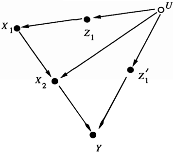
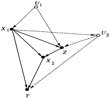
To motivate the discussion, consider an example dis­ cussed in Robins (1993, Appendix 2), as depicted in Figure 1. The variables X 1 and X 2 stand for treat­ ments that physicians prescribe to a patient at two dif­ ferent times, Z represents observations that the second physician consults to determine x2, andy represents the patient's survival. The hidden variables U1 and u2 represent, respectively, part of the patient history and the patient disposition to recover. A simple real­ ization of such structure could be found among AIDS patients, where Z represents episodes of PCP - a com­ mon opportunistic infection of AIDS patients which, as the diagram shows, does not have a direct effect on survival (Y) ( since it can be treated effectively) but is

James Robins

Departments of Epidemiology & Biostatistics School of Public Health Harvard University Boston, MA 02115 robins@hsph. harvard. edu

an indicator of the patient's underlying immune status (U2) which can cause death (Y). X1 and X2 stand for bactrim- a drug that prevents PCP (Z) and may also prevent death by other mechanisms. Doctors used the patient's earlier PCP history (UI) to prescribe X1, but its value was not recorded for data analysis.

The problem we face is as follows. Assume we have collected a large amount of data on the behavior of many patients and physicians, which is summarized in the form of ( an estimated ) joint distribution P of the observed four variables (X1, Z, X2, Y). A new pa­ tient comes in and we wish to determine the impact of the ( unconditional) plan (do(xt), do(x2)) on survival (Y), where x1 and x2 are two predetermined dosages of bactrim, to be administered at two prespecified times.

More generally, our problem amounts to that of evalu­ ating a new plan by watching the performance of other planners whose decision strategies are indiscernible. Physicians do not provide a description of all inputs which prompted them to prescribe a given treatment; all they communicate to us is that U1 was consulted in determining X 1 and that Z and X 1 were consulted in determining X2· But U1, unfortunately, was not

recorded.

The problem of learning from the performance of other planners is that one is never sure whether an observed response is due to the planner's action or due to the event which triggered that action and simultaneously caused the response. Such events are called "con­ founders". The standard techniques of dealing with potential confounders is to adjust for possible varia­ tions of confounders by stratification. This amounts to conditioning the distribution on the various states of the confounding variables, evaluating the effect of the plan in each state separately, then taking the (weighted ) average over those states. However, in planning prob­ lems like the one above stratification is exacerbated by two problems. First, some of the potential confounders are unobservable (e.g., U1), so they cannot be condi­ tioned on. Second, some of the confounders (e.g., Z) are affected by the control variables and, one of the deadliest sins in the design of statistical experiments [Cox 1958, page 48] is to stratify on such variables. The sin being that stratification simulates holding a variable constant, but holding constant a variable that stands between an action and its consequence prevents us from obtaining an accurate reading on the unmedi­ ated effect of that action.

The techniques developed in this paper will enable us to recognize in general, by graphical means, whether a proposed plan can be evaluated from the joint distri­ bution on the observables and, if the answer is positive, which covariates should be adjusted for, and how.

Our starting point is a knowledge specification scheme in the form of a causal diagram, like the one shown in Figure 1, which provides a qualitative summary of the analyst's understanding of the relevant data­ generating processes.1 The semantics behind causal diagrams and their relations to actions and be­ lief networks have been discussed in prior publica­ tions [Pearl & Verma 1991, Goldszmidt & Pearl 1992, Druzdzel & Simon 1993, Pearl 1993a, Spirtes et al. 1993, Pearl 1993b). In Spirtes et al. (1993) and later in Pearl (1993b), for example, it was shown how causal networks can be used to facilitate quantitative predictions of the effects of interventions, including interventions that were not contemplated during the network's construction. A more recent pa­ per [Pearl 1994) reviews this aspect of causal networks, and proposes a calculus for deriving probabilistic as­ sessments of the effects of actions in the presence of unmeasured variables. Using this calculus (reviewed in Appendix I) graphical criteria can be established for deciding whether the effect of one variable (X) on another (Y) is identifiable from sample data involving only observed variables, namely, whether it is possible

1 An alternative specification scheme using counterfac­ tual statements was developed earlier by Robins (1986, 1987), and was used to study the identification problem by non-graphical techniques. Robins' scheme extended Ru­ bin's (1978) counterfactual scheme for singleton actions to compound actions and plans.

to extract from such data a consistent estimate of the probability of Y under hypothetical interventions with variables X. In a related paper [Galles & Pearl 1995) it is shown that the identification of causal effect be­ tween two singleton variables (say X1 and YI) can be accomplished systematically, in time polynomial in the number of variables in the graph.

This paper extends certain results of [Galles & Pearl 1995) to the case where X stands for a compound action, consisting of several atomic in­ terventions which are implemented either concurrently or sequentially. We establish a graphical criterion for recognizing when the effect of X on Y is identifiable and, in case the diagram satisfies this criterion, we provide a closed-form expression for the distribution of an outcome variable Y under the plan defined by the compound action do(X = x ) . The derived expres­ sions invoke only measured probabilities as obtained, for example, by recording past performances of other planning agents or, in case the elements of X are not controlled by agents, by taking passive measurements from the environment. If Y stands for a goal variable, then the formula provides an expression for the proba­ bility that the plan X would lead to goal satisfaction.

2 PLAN IDENTIFICATION

Notation:

A control problem consists of a directed acyclic graph (DAG) G with vertex set V, partitioned into four dis­ joint sets V = {X, Z, U, Y}

• X -represents the set of control variables (exposures, interventions, etc.)
• Z -represents the set of observed variables, often called covariates .
• U -represents the set of unobserved (latent) van­ abies.
• Y - represents an outcome variable.

In this section, we let the control variables be tempo­ rally ordered X= X1, X2, . . . , Xn such that every Xk is an ancestor of Xk+i(j > 0) in G, and we let the outcome Y be a descendent of Xn. We relax these assumptions in Section 6. Let Nk stand for the set of observed nodes that are nondescendents of Xk. A plan is an ordered sequence (x1, x2, . .. , xn) of value­ assignments to the control variables, where Xk means "Xk is set to xk" . A conditional plan is an ordered sequence (g1(z), Y2(z), ... , Yn(z)) where each Yk is a function from Z to X k, and g k ( z) stands for the state­ ment "set Xk to Yk(z) whenever Z attains the value z". The support of each gk(z) function must not con­ tain any z variables which are descendants of xk in G.

Our problem is to evaluate an unconditional plan 2 , namely, to compute P(ylx1, x2, .. . , Xn) which represents the impact of the plan ( x1, . . . , Xn) on the outcome variable Y. The expression P(ylx1, x2, . . . , Xn) is said to be identifiable in G if, for every assign­ ment (.7:1, :1: 2 , ... , .Xn), the expression can be deter­ mined uniquely from the joint distribution of the ob­ servables {X, Y, Z}. A control problem is said to be identifiable whenever P(ylx1, x2, ... , xn) is identifi­ able.

Our main identifiability criteria are presented in Theo­ rems 1 and 3 below. These invoke d-separation tests on various subgraphs of G, defined as follows. Let X, Y, and Z be arbitrary disjoint sets of nodes in a DAG G. We use the expression (X II YIZ)a to denote that the set Z d-separates X from Y in G. We denote by G x the graph obtained by deleting from G all arrows pointing to nodes in X. Likewise, we denote by G x the graph obtained by deleting from G all arrows emerging from nodes in X. To represent the deletion of both incoming and outgoing arrows, we use the notation Gxz· Finally, the expression P(yix, z) � P(y-; zlx)f P(zix) stands for the probability of Y = y given that Z = z is observed and X is held constant at x.

3 ADMISSIBLE MEASUREMENTS

Theorem 1 P(ylx1, . .. , xn) is identifiable if for ev­ ery 1 :::; k :::; n there exists a set Zk of covariates sat­ isfying:

(i.e.' zk consists of non-descendants of xk) and

When the conditions above are satisfied, the plan eval­ uates to3

Before presenting its proof, let us demonstrate how Theorem 1 can be used to test the identifiability of the

2Identification of conditional plans has been con­ sidered in [Robins 1986, 1987] and certain extensions of our graphical results are presented in [Pearl 1994, Robins & Pearl 1995].

3The computation and estimation of sum-product ex­ pressions of the form given in Eq. (3), where Z" stand for any subset of Nk, were investigated by J. Robins under the rubric "G-computation algorithm formula" [Robins 1986], hereafter G-formula.

control problem shown in Figure 1. First, we will show that P(yix1, x2) cannot be identified without measur­ ing z, namely, the sequence z1 = {0}, z2 = {0} would not satisfy conditions (1)-(2). The two d-separation tests encoded in (2) are:

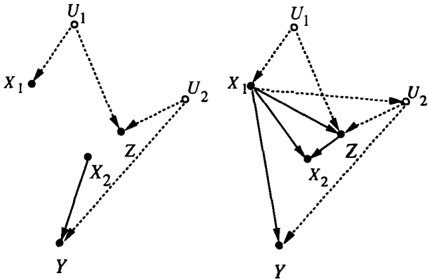
The two subgraphs associated with these tests are shown in Figure 2, (a) and (b), respectively. We see

that, while (Y II X1) holds in Gx x , (Y II X2IX!) --1' 2 -fails to hold in Gx . Thus, in order to pass the test, -2 we must have either Z 1 = {Z} or Z2 = {Z} but, since Z is a descendant of X 1, only the second alternative remains: Z2 = { Z}. The test applicable to the se­ quence zl = {0}, z2 = {Z} are: (Y II Xt)a --�l,X2 and (Y II X2IX1, Z)ax . Figure 2 shows that both --2 tests are now satisfied, because {X 1, Z} d-separates Y from X2 in Figure 2(b ). Having satisfied conditions (1)-(2), Eq. (3) provides a formula for the effect of plan (x1, x2) on Y:

The question naturally arises whether the sequence Z1 = {0} Z2 = {Z} can be identified without exhaus­ tive search. This will be answered in Corollary 2 and Theorem 3.

Proof of Theorem 1: The proof given here is based on the inference rules described in Appendix I which facilitate the reduction of causal-effect formulas to hat­ free expressions. An alternative proof is provided in Section 6. 1.

1. The condition Zk C Nk implies Zk � Ni for all j 2: k. Therefore, ;-e have

This is so because no node in {Z1, ... , Zk, X1, ... , Xkd can be a descendant of any node in {Xk, ... , Xn}, hence, Rule 3 al­ lows us to delete the hat variables from the ex­ presswn.

1. Condition (2) permits us to invoke Rule 2 and write:

Thus, we have

0

Definition 1 Any sequence Z1, ... , Zn of covariates satisfying conditions (1) and ( 2 ) will be called "admis­ sible" and any expression P(yl!i:1, !i:2, ... , !i:n) which is identifiable by the criterion of Theorem 1 will be called G-identifiable.

An immediate corollary of the definition above is

Corollary 1 A control problem is G-identifiable if it has an admissible sequence.

G-identifiability is sufficient but not necessary for plan identifiability as defined above ( see also Definition 3, Appendix I). The reasons are two fold. First, the com­ pleteness of the three inference rules used in the reduc­ tion of ( 3) is still a pending conjecture. Second, the kth step in the reduction of ( 3) refrains from condi­ tioning on variables Zk that are descendants of Xk; namely, variables that may be affected by the action d o (Xk = xk) · In certain causal structures, the identi­ fiability of causal effects requires that we condition on such variables [Pearl 1994].

Theorem 1 provides a declarative condition for plan identifiability. It can be used to ratify a proposed causal effect formula for a given plan, but does not provide an effective procedure for deriving such for­ mulas, because the choice of each Zk is not spelled out procedurally; the possibility exists that some choices of Zk, satisfying (1) and (2), might prevent us from continuing the reduction process even in cases where such reduction exists.

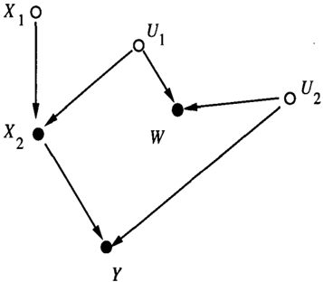
This is illustrated in Figure 3. Here W is an ad­ missible choice for zl' but if we make this choice we will not be able to complete the reduction, since no set Z2 can be found that satisfies condition (2): (Y II X2IX1 . W, Z2)G _ . In this case it would be -K2, xl wiser to choose zl = z2 = 0, which satisfies both: (Y II Xll0)ax , and (Y II X2 I X1,0)a -. --1 -_K2Xl

y

Figure 3: Illustrating an admissible choice Z1 that rules out any admissible choice for z2. w

4 EVALUATION BY G-FORMULA

Let Lk consist of all non descendants of Xk which are descendants of Xk-l, including both observed and un­ observed variables but exclusive of the controlled vari­ ables. Robins [1987] has shown, using counterfactual analysis, that

and named (5) the G-formula based on L1, ... , Ln. One way of verifying (5) is to write the post­ intervention distribution on all uncontrolled variables (using (18))

then take the marginal distribution on Y by summing on the lk 's. The identity of (6) and (5) follows from the independence

Upon explicating the lk 's in (5), we may find that some factors contain latent variables. When this happens we may try to use the conditional independencies encoded in the graph to eliminate those latent variables and, if we succeed, the plan would be identifiable and the resulting formula would give the desired causal effect.

Let us demonstrate this method on the example of Figure 1. The Lk sequence is given by L1 = {UI} and L 2 = {Z, U2}. Substituting in the G-formula yields.

Using the graph independencies (Y II {Z,UI}I{X1,X2,U2})a and (U2 _ II U1IXI)a, we g cl

which agrees with ( 4) under the admissible sequence Z1 = 0 Z2 = Z. Thus, by succeeding to eliminate the U variable from the G-formula, we obtain a confir­ mation of plan identifiability together with the correct causal effect estimands.

The elimination method above still requires some search and algebraic skill. In addition, when the num­ ber of latent variables increases, the expressions tend to become rather involved. We now return to the prob­ lem of finding an admissible sequence, if one exists, thus eliminating the search altogether.

5 FINDING AN ADMISSIBLE SEQUENCE

The obvious way to avoid bad choices of covariates, like the one illustrated in Figure 3, is to insist on always choosing a "minimal" Zk, namely, a set of covariates

satisfying (2) having no proper subset which satisfies (2). However, since there are usually a large number of such minimal sets ( see Figure 4), the question re­ mains whether every choice of a minimal Zk is "safe", namely whether we can be sure that no choice of a minimal subsequence zl' ... ' zk will ever prevent us from finding an admissible zk+l' in case some admis­ sible sequence Zi, ... , Z� exists.

The next result guarantees the "safety" of every min­ imal subsequence zl' ... ' zk and, hence, provides an effective test for G-identifiability.

Theorem 2 If there exists an admissible sequence Zi, ... , Z�, then for every minimally admissible subse­ quence Z1, ... , Zk-l of covariates, there is an admis­ sible set Z k.

Proof: The proof will be based on Lemmas 1 and 2 which are proved separately in Appendix II.

Lemma 1 For any DAG G and any two disjoint sub­ sets of nodes X and Y , let the ancestor-set of (X, Y), denoted A ( X, Y), be the set of nodes which have a de­ scendant in either X or Y .

The following two separation conditions hold for any sets of nodes W and Z:

Eq. ( 8) asserts that conditioning on nodes from an ancestral set can only create, never destroy indepen­ dencies. Eq. (9) asserts that conditioning on all the nodes outside the ancestral set can only destroy, never create independencies.

Lemma 2 Denote by Gk the subgraph G 14, xk + 1 , · . . , Xn ofG, and let Ak be the ancestral set of(Xk, Y) in Gk. For any j > 0, Ak is a subset of the ancestral set of (Xk. Y) in Gk+i.

We now prove Theorem 2 by contradiction. Suppose that Z1, ... , Zk_1 is minimally admissible sequence, and that no admissible set Zk exists. This means, in particular, that the set Zk = Ak n Nk is inadmissible, I. e.,

Now observe that no node in the sequence Z1, ... ,Zk-1 can reside outside Ak nNk. This is so because admissibility dictates Z; E N; and

so, the lowest i for which Z; contains a nonmember of Ak will violate minimality (by (9)). Indeed, Lemma 2 insures that the violating Z; must also contain non­ members of A; (in G;) , and (9) implies that if we re­ move all non-A; from a conditioning set, we do not de­ stroy any separation. Moreover, since such a removal from {X1, ... , X; _1, Z1, ... , Z;} will only affect Z;, we can substitute A; for Z; in Eq. (11). This implies that A satisfies (2) and Z; is non-minimal, which is a con­ tradiction. We are now assured that Z1, ... , Zk-1 are in Ak n Nk. Likewise, since {X1, .. . , Xk-d is also in Ak n Nk. (10) can be rewritten as

To prove that (10) is false, contrast (12) with the assumption that there exists an admissible sequence zr, ... ,z�. Let Z* = zzu :,:} (Zi U {X;}). Admis­ sibility states that (2) is satisfied by zk = z;' hence, (Y II Xk IZ*)ak. By (9), we can intersect the conditioning set Z* with Ak, yielding (Y II xk IZ* n Ak)· Finally, since Z* � Nk, we have -

But (12) and (13) together contradicts (8), because (8) asserts that whenever we add to the conditioning set members of Ak, we preserve independencies. QED

Theorem 2 now provides an effective decision proce­ dure for testing G-identifiability:

Corollary 2 A control problem is G-identifiable if and only if the following algorithm exits with success:

1. Set k = 1
2. 2 . Choose any minimal Zk E Nk satisfying {2 ),
3. If no such Zk exists, exit with failure. Else set k = k + 1,
4. If k = n + 1, exit with success, else go to step 2 .

From the proof of Theorem 2, it is obvious that we need not insist on choosing minimal Zk. That re­ quirement only insures that we do not step outside Ak and spoil the selection of future subsets. In fact, Lemma 1 guarantees that if an admissible sequence exists, then W1, W2, ... , Wn is such a sequence, where Wk = Ak n Nk. Accordingly, we can now rewrite The­ orem 1 in terms of an explicit sequence of covariates.

Theorem 3 P(yl:h, ... , Xn) is G-identifiable if and only if the following condition holds for every 1 ::; k ::; n

where Wk = Ak n Nk , namely, Wk is the set of all covariates in G that are both non-descendants of Xk and have either Y or Xk as descendant. Moreover, when the condition above is satisfied the plan evaluates to

6 GENERALIZATIONS

6.1 Y AND Z NON-DISJOINT

In practice, we will often be interested in a vector out­ come Y with components of Y being ancestors of con­ trol variables Xk for some k. For instance, in our AIDS example, we may be interested in survival Y not only at a time after subjects have received treatment x2 but also at a time after receiving treatment x1 but before receiving X 2. If a component of Y is both an ancestor of a control variable Xk and of a later component of Y, it is necessary to regard the former component as a confounding variable that must be adjusted for to esti­ mate the effect of the plan on Y. To do so, we no longer impose the assumption that Y is a descendent of Xn and that Y and Z are disjoint. Rather, we shall only require that Y C Z where, henceforth, Z represents all observed non-control variables. With this redefinition of Y, with the understanding that (Y II XIX)a VX, we prove below that -

Theorem 4 Given Y C Z, Theorem 1 remains true .

Further, under the above redefinitions of Y and Z, we also obtain a natural generalization of Theorem 3. Let Y; be the subset of Y that is not in Nk and let Yk be the subset of Y that is in Nk. Redefine Ak to be the ancestral set of (Xk, Yn in graph Gk. Robins and Pearl (1995) prove

Theorem 5 : Given Y C Z, Theorem 3 remains true with Wk redefined to be (AknNk ) UYk.

A key step in the proof of Theorem 5 is the following Lemma proved in [Robins & Pearl 1995).

Lemma 3 If a sequence Zk is G-admissible, then the sequence Zk u Y k is also G-admissible .

We shall also need this Lemma 3 in Section 6.3 below.

Proof of Theorem 4: Given a plan x = (x1, ... , xn), define

To prove Theorem 4, we shall use the following Lemma which is an easy consequence of the corollary to The­ orem ( AD.1) in Robins (1987).

Lemma 4 If, for each k, Zk c Nk and the expression

does not depend on xk then Eq. {3) is true.

One can also prove Lemma ( 4) directly by using induc­ tion on n to show that the right hand side of Eq. (5) plus the premise of the lemma imply the right hand side of Eq. (3).

To complete the proof of Theorem 4, we shall show that (i) the premise of Lemma (4) is equivalent to the statement that

when probabilities are computed under a particular joint distribution Pkx for the variables V in G and (ii) Pkx is represented by the DAG G k = G�,xk+1, ... ,Xn [i.e. ' by definition, Pkx ( v) = n j Pkx ( Vj I paj k) where Pajk are the parents of Vj on Gk and pajk is the value of Pajk when V = v]. It then follows that Eqs. (1) and (2) imply the premise of Lemma ( 4), proving Theorem 4.

Let P denote the distribution of variables V on G. Now, given a plan x = (x1 ... xn), define Pkx (v) = Tij Pkx(Vj IPajk) where (i) if Vj = Xm for some m, m = k + 1, ... , n, then Pkx(Vj IPajk) = 1 if Vj = Xm, and (ii) if Vj =/= Xm for m = k + 1, . . . , n, Pkx(Vj IPajk) = P(vj IPajk) when xk is not a parent of Vj on G, and Pkx (vj I pajk) = P(vj I xk = Xk,pajk) when xk is a parent of Vj on G. By construction, Pkx is represented by the DAG G k and, therefore, xk l1 y I £1, 0 0 0' Lk, xl, 0 0 0 ' Xk-1 un­ der the distribution Pkx · Further, it is straightforward to calculate that (i) for any xk, h(y I x, £1, ... , fk) = Pkx(Y I xl = Xl, ... ,Xk-1 = Xk-1, xk = xk, £1 = £1, ... ,Lk = fk), and (ii) the conditional dis­ tributions of £1, ... , Lk given (Z1, ... , Zk, X1, ... , Xk) are the same under P and Pkx· Hence, the premise of Lemma ( 4) is equivalent to the conditional indepen­ dence under the distribution Pkx of Y and Xk given (Zl, ... ,Zk,Xl = Xl, ... ,Xk-1 = Xk-1)·

We note that the premise of Lemma (4) is a non­ graphical condition that is weaker than the graphical premise of Theorem 4 and yet implies identifiability by the G-formula based on Z1, ... , Zn. However, as a non-graphical condition, the premise of Lemma ( 4) is much more difficult to check that the graphical premise of Theorem 4.

6.2 Xk+j NEED NOT BE A DESCENDENT OF Xk

In this subsection, we relax the assumption that Xk+j is a descendent of Xk for all k,j > 0 . As in Sec. 6.1, Z remains the set of all observed non-control vari­ ables. Given X C V, we say X = (X1, ... , Xn) is consistent ordering of X in G if, for each k, Xk is a non-descendent of {Xk+1, ... ,Xn}· Hence­ forth, given a consistent ordering of X, we redefine Nk to be the set of observed non-control variables that are non-descendents of any element in the set {Xb Xk+1, ... , Xn}· Robins and Pearl (1995) proved

Theorem 6 Given a consistent ordering (X1, ... , Xn) of X with Xk not necessarily an ancestor of Xk+i, Theorems 4 and 5 remain true.

Theorem 6 is an immediate corollary of Theorems 4 and 5, and the following Theorem proved in Robins and Pearl (1995) characterizing arrows that can be added into and out of the xk without destroying Eqs. (1) and (2). Given a graph G, a consistent order­ ing (X1, ... ,Xn) of X, and sets Z1, ... ,Zn,Zk C Nh let graph G* be the graph in which, for each k, all ar­ rows are included (i) from Xk both to each member of the set {X k+l, ... , Xn} and to each variable (observed or unobserved) that is a descendent of some member of { Xk+l, ... , Xn} and (ii) from each member of the set zl u 0 0 .uzk to xk.

Theorem 7 Eqs . {1}-{2} hold for graph G if and only if Eqs . {1}-{2} hold for graph G*.

Robins and Pearl (1995) show that the choice of con­ sistent ordering for X does matter. Specifically, they provide an example with X = (X a, X b ) bivariate in which both the ordering (X1,X2) = ( Xa,Xb ) and the ordering (X 1, X 2) = (X b, X a ) are consistent orderings of X. However, p (y I x) is only G-identifiable based on the ordering X = ( Xb, Xa ) ·

6.3 VARIABLES THAT CAN BE DISCARDED

Eqs. (1)-(2) provide sufficient conditions for a­ identification solely in terms of associations between observed variables. In the epidemiologic literature, sufficient conditions for G-identification are often ex­ pressed in terms of associations between unobserved and observed variables. For example, for the ef­ fect of a singleton action X on Y, it is a stan­ dard result that an unobserved non-descendent of X, say U, is a "non-confounder given data on a non­ descendent zl of X" [i. e. , p (y I x) is G-identifiable based on Z1] if either U and X are conditionally in­ dependent given zl or if u and y are conditionally independent given (Z1, X) [Miettinen & Cook 1981, Robins & Morgenstern 1987,

Greenland & Robins 1986]. Extensions to compound actions are discussed in Robins (1986, Sec. 8 and Ap­ pendix F; 1989) and Robins et al. (1992, Sec. A2. 13). The following theorem recasts Theorem 4 into this more familiar epidemiologic form. Given Z1, ... , Zn with Zk c Nk, let u; be all non-descendents of {Xk, . . . , Xn} (observed and unobserved) that are both non-control variables and are disjoint from Z1, ... , Zk. Robins and Pearl (1995) prove

Theorem 8 Suppose that, for each k, Yk c Zk · Then Eqs. {1}-{2} hold if and only if, for each k, u; = (U;k , u; k ) for (possibly empty ) disjoint sets u:k, u;k satisfying

• (i) and

(ii) (U;kUYk' IXl, ... , xk ,zl, ... ,zk,u; k )a_ _ . Xk+l, ... ,Xn Note that, in view of Lemma 3, the assumption Yk C Zk is completely non-restrictive since we can always replace zk by zk UYk without destroying Eq. (1) or Eq. (2).

An important issue not treated in this paper is to derive sufficient conditions for the identification of p (y I x) when p (y I x) is not G-identifiable. Robins and Pearl (1995) provides sufficient conditions for identification of nan-G-identifiable effects p (y I x). When these criteria are satisfied, they provide a closed­ form expression, called the composite-G-formula, for P(y 1 x).

Acknowledgment

Professor Pearl's research was partially supported by Air Force grant # AFOSR/F496209410173, NSF grant #IRI-9420306, and Rockwell/Northrop Micro grant #94-100 and Professor Robins' research was supported by NIH grant # R01-AI32475.

References

• [Cox 1958] Cox, D.R. (1958) The Planning of Exper­ iments . New York: John Wiley and Sons.

[Druzdzel & Simon 1993] Druzdzel, M.J . , and H.A. Simon (1993) Causality in Bayesian Be­ lief. In Proceedings of the Ninth Confer­ ence on Uncertainty in Artificial Intelli­ gence (eds. D. Heckerman and A. Mam­ dani), CA, 3-11.

[Galles & Pearl 1995] Galles, D. and J. Pearl (1995) Testing identifiability of causal effects. Technical Report R-226, UCLA Cogni­ tive Systems Laboratory. To appear m UAI-95.

[Goldszmidt & Pearl 1992] Goldszmidt, M., and J. Pearl (1992) Default Ranking: A Practi­ cal Framework for Evidential Reasoning, Belief Revision and Update. In Proceed­ ings of the Third International Confer­ ence on Know/edge Representation and Reasoning, 661-672.

• [Greenland & Robins 1986] Greenland, S., and J . M . Robins (1986) Identifiability, Ex­ changeability and Epidemiologic Con­ founding. International Journal of Epi­ demiology, 15, 413-419.

[ Miettinen & Cook 1981] Miettinen, O.S., and E.F. Cook (1981) Confounding essence and detection. American Journal of Epi­ demiology, 114, 593-603.

[Pearl 1993a] Pearl, J. (1993a) From Conditional Oughts to Qualitative Decision Theory. In Proceedings of the Ninth Conference on Uncertainty in Artificial Intelligence (eds. D. Heckerman and A. Mamdani), 12-20.

• [Pearl 1993b] Pearl, J. (1993b) Graphical Models, Causality, and Intervention. Statistical Science, 8(3), 266-273.

[Pearl 1994] Pearl, J. (1994) A Probabilistic Calculus of Actions. In Proceedings of the Tenth Conference on Uncertainty in Artificial Intelligence ( eds. R. Lopez de Mantaras and D. Poole), 454-462.

• [Pearl 1995] Pearl, J. (1995) Causal Diagrams for Ex­ perimental Research. Technical Report R-218-B, UCLA Cognitive Systems Lab­ oratory. To appear in Biometrika .

[Pearl & Verma 1991] Pearl, J., and T. Verma (1991) A Theory of Inferred Causation. In Prin­ ciples of Know/edge Representation and Reasoning: Proceedings of the Second In­ ternational Conference ( eds. J .A. Allen, R. Fikes, and E. Sandewall), 441-452.

[Robins 1986) Robins, J.M. (1986) A new approach to causal inference in mortality studies

with a sustained exposure period - appli­ cations to control of the healthy workers survivor effect. Mathematical Mode/ling, 7, 1393-1512.

• [Robins 1987] Robins, J.M. (1987) Addendum to "A new approach to causal inference in mor­ tality studies with a sustained exposure period applications to control of the healthy workers survivor effect". Com­ puters and Mathematics with Applica­ tions, 14, 923-945.
• [Robins 1989] Robins J.M. (1989) The control of confounding by intermediate variables. Statistics in M edicine,8 , 679-701.
• [Robins 1993] Robins J.M. (1993) Analytic methods for estimating HIV treatment and co­ factor effects. In: Methodological Issues of A IDS Mental Health Research (eds. D.G. Ostrow, R. Kessler) New York: Plenum Publishing, 213-290.
• [Robins & Morgenstern 1987] Robins J.M., and H. Morgenstern (1987) The Foundations of Confounding in Epidemiology. Com­ puters and Mathematics with Applica­ tions, 14, 869-916.
• [Robins & Pearl 1995] Robins, J., and J. Pearl (1995) Causal Effects of Dynamic Policies. In preparation.
• [Robins et al. 1992] Robins, J .M., D. Blevins, G. Ritter, and M. Wulfsohn (1992) G­ estimation of the effect of prophylaxis therapy for pneumocystis carinii pneu­ monia on the survival of AIDS patients. Epidemiology, 3, 319-336.
• [Rubin 1978] Rubin, D.B. (1978) Bayesian Inference for Causal Effects: The Role of Random­ ization. The Annals of Statistics, 6, 3458.
• [Spirtes et al. 1993] Spirtes, P., C. Glymour, and R. Schienes (1993) Causation, Predic­ tion, and Search. New York: Springer­ Verlag.

APPENDIX I

This appendix summarizes the basic definitions, no­ tations and inference rules used in the body of the paper. Details and proofs can be found in [Pearl 1994, Pearl 1995].

Let V = { V1 , V2, ... , Vn} be the set of all variable in a directed acyclic graph ( dag) G.

Definition 2 (causal effect) Given two disjoint sets of variables, X and Y, the causal effect of X on Y, denoted P(ylx), is a function from X to the space of probability distributions on Y. For each realization x of X, P(ylx) gives the probability of Y = y induced by the action do( X = x ) .

If causal knowledge is organized as a set T of structural equations

where pa; are the parents of X; in G, f; are ( un­ specified) deterministic functions and f; are mutually independent disturbances [Pearl & Verma 1991], then the joint distribution of the observed variables has the product from

independent of the f; 's in T. In such a process-based theory, the effect of the action do(Vj = vj) amounts to overruling the process governed by f; and substituting the process Vj = v� instead. Consequently, the induced distribution in the mutilated theory Tv ' would be J

independent ofT. The partial product reflects the re­ moval the factor P(vJIPa;) from the product of (16). Multiple actions result in the removal of the corre­ sponding factors from (16).

Definition 3 (identifiability) The causal effect of X on Y is said to be identifiable if the quantity P(ylx) can be computed uniquely from any positive distri­ bution of the observed variables. In other words PT,(Yix) = PT2(ylx) whenever PT,(v) = PT2(v) > 0.

Identifiability means that P(ylx) can be estimated consistently from an arbitrarily large sample randomly drawn from the distribution of the observed variables.

The following theorem states the three basic inference rules used in the text.

Theorem 9 Let G be the directed acyclic graph asso­ ciated with a causal model, and let P( · ) stand for the probability distribution induced by that model. For any disjoint subsets of variables X, Y , Z, and W we have:

Rule 1 Insertion/ deletion of observations

Rule 2 Action/ observation exchange

一

Rule 3 Insertion/ deletion of actions

ancestors of any W-node in Gx·

Each of the inference rules above follows from the ba­ sic interpretation of the " x" operator as a replacement of the causal mechanism that connects X to its pre­ action parents by a new mechanism X = x introduced by the intervening force. The result is a submodel characterized by the subgraph Gy (named "manipu­ lated graph" in Spirtes et al. (1993)) which supports all three rules.

Rule 1 reaffirms d-separation as a valid test for condi­ tional independence in the distribution resulting from the intervention se t (X = x ) , hence the graph Gx· This rule follows from the fact that deleting equations from the system does not introduce any new depen­ dencies among the remaining variables.

Rule 2 provides a condition for an external interven­ tion do( Z = z ) to have the same effect on Y as the passive observation Z = z. The condition amounts to {X U W} blocking all back-door (i.e., spurious) paths from Z to Y (in Gx ) , since Gyz retains all (and only) such paths. -

Rule 3 provides conditions for introducing (or delet­ ing) an external intervention do( Z = z ) without af­ fecting the probability of Y = y. The validity of this rule stems, again, from simulating the intervention do( Z = z ) by pruning all links entering the variables in Z (hence the graph Gxz ) ·

Corollary 3 A causal effect q: P(yl,···,Ykl xl, ... , xm) is identifiable in a model characterized by a graph G if there exists a fi­ nite sequence of transformations, each conforming to one of the inference rules in Theorem 9, which reduces q into a standard (i.e., hat-free) probability expression involving observed quantities. 0

APPENDIX II

Proof of Lemma 1

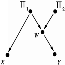
We will prove (8) by showing that if (Y II XIZ)a holds, then augmenting Z by any additional node w E A(X, Y) preserves the separation between X and Y. Assume w is an ancestor of Y. If (Y II XIZ)a is true and (Y II XIZ, w )a is false, then there must be a path between a node in X and Y that is blocked by Z and become unblocked by Z U { w }. Let 1r1 and 1r2 be two parents of w which became dependent by conditioning on w and assume 1r1 d-connects to X.

X

Figure 5:

Since all paths were blocked prior to conditioning on w, it must be that all paths from w to Y are blocked as well. But, since w is an ancestor of Y, this means that some member of Z resides on a directed path from w to Y. This, however, means that 1r1 and 1r2 were not d-separated prior to conditioning on w; thus contradicting our basic assumption that conditioning on w opened a new pathway between X and Y. A symmetrical argument applies if w is an ancestor of X (or of both). Repeating the proof for each w E A(X, Y) completes the proof of (8).

To prove (9), we show that any path p between X and Y that is blocked by W will remain blocked when we remove from W all nodes that are descendant of either X or Y. Indeed, in order to unblock a path p by re­ moving nodes from W some of the removed nodes must be non-colliders on p. Now, if p is totally in A( X, Y) no node on p will be removed. On the other hand, if p has some nodes outside A(X, Y), it must have at least one collider c, such that c and all its descendants are outside A(X, Y). Therefore, when we remove from W all non-ancestral nodes, we must leave c and all its descendant unconditioned, hence p must remain un­ blocked. QED

Proof of Lemma 2

We shall first prove that any ancestor of (Y , X;) in G; is also an ancestor of (Y , X;) in Gi+j. 1ft is an ancestor of X; in G; then clearly it must be an ancestor of X; in G;+i; going from G;+i to G; does not affect any path incoming to X;. Now assume that tis an ancestor of Y in G; but not in Gi+j. This can only happen if all paths (in G ) from t to Y go through Xi+i and get blocked in G; by removing the outgoing arrows from X;+i. But any such path will be blocked in G; as well, because all incoming arrows to Xi+i are removed in G;, hence, t cannot be an ancestor of Y in G;, which is a contradiction. We conclude that any ancestor of Y in G; must also be an ancestor of Y in Gi+l· Combining the two cases, completes the proof of Lemma 2.

(Remark: This proof relies on the assumption that each Xk+i is an ancestor of X k . )