Probabilistic Inference in Influence Diagrams

Nevin Lianwen Zhang

Department of Computer Science, Hong Kong University of Science & Technology lzhang�cs.ust.hk

Abstract

This paper is about reducing influence dia­ gram (ID) evaluation into Bayesian network (BN) inference problems. Such reduction is interesting because it enables one to read­ ily use one's favorite BN inference algorithm to efficiently evaluate IDs. Two such reduc­ tion methods have been proposed previously (Cooper 1988, Shachter and Peot 1992). This paper proposes a new method. The BN in­ ference problems induced by the mew method are much easier to solve than those induced by the two previous methods.

Keywords: Decision analysis, influence diagrams, Bayesian networks, inference.

1 Introduction

Influence diagrams (IDs) (Howard and Matheson 1984) are a popular framework for decision analysis. An ID is an acyclic graph with three types of nodes: random nodes, decision nodes, and a single value node. Each random node is associated with a conditional probability table (CPT) and the value node is associ­ ated with a utility function. Evaluating an ID means finding an optimal decision rule for each of its decision nodes.

IDs without decision and value nodes are called Bayesian networks1 (BNs) (Pearl 1988). They are widely used by AI researchers as a knowledge repre­ sentation framework for reasoning under uncertainty. There is a rich collection of exact and approximate al­ gorithms for inference in BNs. This paper is about how to reduce ID evaluation into BN inference prob­ lems that are as easy to solve as possible. Such re­ duction is interesting because it enables one to readily

1 Also known as belief networks and probabilistic influ­ ence diagrams.

use one's favorite BN inference algorithm to efficiently evaluate IDs.

Cooper (1988) initiated research in this direction. He proposed a transformation of an ID into a BN and showed that optimal decision rules can be found by posing an appropriate sequence of queries to the BN. Several improvements were later introduced by Shachter and Peot (1992). This paper proposes a new method. The BN inference problems induced by the new method are much easier to solve than those in­ duced by the two previous methods.

There are several algorithms that evaluate IDs di­ rectly without the reduction into BN inference prob­ lems (Shachter 1986, Shenoy 1992, Ndilikilikesha 1994, and Jensen et al 1994). We call them direct evalua­ tion algorithms. An method that reduces ID evalua­ tion into BN inference problems would be unattractive if, no matter what BN inference algorithms are used, it is less efficient than the best direct evaluation al­ gorithm. We show that the performance of our new method, when coupled with a BN inference algorithm called VE (Zhang and Poole 1996), is always within a constant factor of the performance of the best direct evaluation method and argue that it is usually more efficient.

The fact that arbitrary BN inference algorithms can used for probabilistic calculations makes our method very attractive as compared to direct evaluation algo­ rithms. From a system development point of view, the method enables one to easily add ID evaluation capa­ bilities to any BN inference packages. From the effi­ ciency point of view, speeding up inference in BNs has been and still is an active research area. There are al­ gorithms that exploit independence of causal influence (e.g. Zhang and Poole 1996) and that exploit special structures in the conditional probability tables. The new method facilitates ready incorporation of those al­ gorithms, as well as future advances in BN inference, in ID evaluation. We are not aware of any approximate algorithms for IDs, while there is a rich collection of

approximate and simulation algorithms for BNs. The new method also opens up the possibility of approxi­ mate algorithms for ID, which might be necessary in order to solve large decision problems.

We will begin with definitions related to influence diagrams and a brief review of Shachter and Peot's method (Section 2). Foundations for our new method will be laid in Section 3 and details will be worked out in Section 4. The new method will be illustrated through an example in Section 5 and compared with Shachter and Peot's method and direct evaluation al­ gorithms in Section 6. Conclusions will be drawn in Section 7.

2 Influence diagrams

In the original definition of IDs (Howard and Math­ eson 1984), there is only one value node. We allow multiple value nodes here so that separability in the utility function can be represented. See Tatman and Shachter (1990) for discussions on separability of util­ ity functions.

IDs are required to satisfy several constraints. First, value nodes cannot have children. Second, IDs must be regular in the sense that there must be a directed path that contains all the decision nodes. The last decision node on the path will be referred to as the tail decision node. Third, they must be no-forgetting in the sense that a decision node and its parents be parents to all subsequent decision nodes. The rationale behind the no-forgetting constraint is that information available now should also be available later if the decision-maker does not forget.

Value networks refer to IDs that do not contain de­ cision nodes. Bayesian networks (BNs) (Pearl 1988) are IDs that consists of only random nodes. In the following, the terms "nodes" and "variables" will be used interchangeably.

We shall use Ox to denote the frame of variable x, i.e. the set of possible values of x. For a set X of variables, Ox stands for the Cartesian product I1xEX n,.

Let d1, .. . , dk be all the decision nodes in an ID N. A decision rule for a decision node di is a mapping 8i : Dnd· --+ n d i . A policy is a list of decision rules � = ( 81: . . . , 8k) consisting of one rule for each decision node. To evaluate an ID is to find an optimal policy that maximizes the expected utility and to compute the optimal expected utility.

ID evaluation requires a lot of probabilistic calcula­ tions. This paper is concerned with identifying a set of probabilistic inference problems such that optimal decision rules can be readily obtained from their so- lutions. The problems should be as easy to solve as possible.

Cooper (1988) initiated research in this direction. Sev­ eral improvements to Cooper's method were proposed by Shachter and Peot (1992). This section briefly re­ views the method by Shachter and Peot.

The method applies only in the case when there is one value node. Let N be an ID with one value node. Denote the value node by v. For simplicity, assume that the utility function fv(7rv) of v is non-negative2· The node is converted into a binary random node with the following conditional probability:

where Mv = maxnvfv(7rv). This transformation will be referred to as Cooper's transformation.

Each decision node d is also converted into a random node with the following conditional probability:

for each possible value a of d, where IDdl is the number of possible values of d. After the transformations, N becomes a BN. Denote the BN by N'.

According to the regularity constraint, there exists a directed path that contains all decision nodes. Let d1, .. . , dk an enumeration of the decision nodes in the order they appear in the path. It is shown that an optimal decision rule t5k, for dk can be obtained by

After the rule has been computed, the conditional probability of dk is changed to Po ;. ( dk j1r dk). An op­ timal decision rule for dk-l is then computed using the same formula except with k replaced by k-1. Op­ timal decision rules for dk-2, . .. , d1 are computed recursively in the same fashion.

Shachter and Peot's method reduces the evaluation of N into the following BN inference problems:

We will show that an ID can be evaluated by solving BN inference problems that are much easier than those listed above.

2If the utility function takes negative values, a constant can be added to it so that it takes only non-negative val­ ues. Addition of a constant to the utility function does not change the optimal policies. Moreover, the optimal ex­ pected value of an ID equals to its optimal expected value after the addition of the constant minus the constant.

3 Decomposition theorem

Suppose N is an ID and d is the tail decision node. This section shows that N can be decomposed into two components, called tail and body respectively, such that an optimal decision rule for d can be found in the tail and optimal decision rules for all other decision nodes can be found in the body. The body is again an ID and hence the decomposition can be repeated in the body.

3.1 Downstream and upstream sets

We begin by partitioning the set of nodes in N into several subsets w.r.t to the tail decision node d. The moral graph of an ID is obtained by first adding undi­ rected edges between pairs of parents of each node so that they are pairwise connected and then dropping directions of all the directed edges. Let x and y be two nodes and S be a set of nodes that does not con­ tain x or y. We say that S m-separates x and y if, in the moral graph, every path connecting them contains at least one node in S.

Let X be the set of all nodes in an ID N. The up­ stream set of N w.r.t to d, denoted by X1, is the set of nodes in X\7rd that are m-separated from d by 1l"d· The downstream set of N w.r.t d, denoted by Xz, is the set of nodes in X\7rd that are not m-separated from d by 1rd· Note that dEXz and that the three sets X1, 7rd and X2 constitute a partition of the set X.

Define 1r d 2 be the set of nodes in 1r d that have at least one pare � t in X2 and set 7rd ,l =7rd\7rd,2· The four sets X1, X2, 1l"d,b and 7rd,z constitute another partition of X.

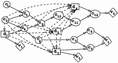
Consider the ID in Figure 1. The set of parents of dz is 7rd2 ={dbc3,c4} and the downstream set Xz w.r.t d2 is X2={d2,c6,vz}. Since c4 the only parent of d2 that has a parent in the downstream set, 7rd2,z={c4}· Hence 7rd2,1 = {d1,c3}.

A node x is an ancestor to another node y if there is a directed path from x to y. A ancestral set an( A ) of a

set of nodes A consists of nodes in A and their ances­ tors. The following proposition summarizes properties of the aforementioned sets.

Proposition 1 Suppose d is the tail decision node in an ID. Then {1) the node d is the only decision node in the downstream set Xz;{2) all nodes in 7rd,2 are random nodes; {3) all nodes in an(7rd,z)nXz are random nodes; and (4) all other decision nodes are in 7rd, l·

3.2 Bodies and tails

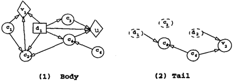
The body of N w. r. t d is an ID given by:

Procedure body(N, d):

1. Prune from N all the nodes in Xz \an(7r d,2)·
2. Return the resulting ID.

We use B to denote the body. According to Proposi­ tion 1 (4), for any decision node d1-:j:.d, d1 is in B and it has the same parents in B as in N.

Define the tail of N w.r.t d by the following procedure:

Procedure tail(N, d):

1. Prune from N all nodes in X 1·
2. Prune arcs into d and nodes in 1r d, l ·
3. Prune conditional probabilities of ran­ dom nodes in 1r d,l·
4. For each node xE{d}U7rd,l, set P.r(x)=l/lf!xl, where lf!xl is the num­ ber of possible values of x.
5. Convert all the value nodes in Xz into random nodes by Cooper's transforma­ tion.
6. Return the resulting BN.

We use T to denote the tail. It is a BN for the fol­ lowing reasons. It consists the decision node d, nodes in 7rd,1, nodes in 1rd,2UX2\{d}. The node d and nodes in 1r d 1 are associated with uniform distributions. Ac­ cordi � g to Proposition 1, nodes in 1rd,2UX2\{d} are either random nodes or value nodes. Random nodes in the set inherit their conditional probabilities from N, while conditional probabilities for value nodes in the set are obtained from their utility functions via Cooper's transformation. So all nodes in T are asso­ ciated with probabilities and hence T is a BN.

Let V2 be the set of all value nodes in the tail. Define the evaluation functional er(7rd, d) of the tail T by

3.3 Decomposition theorem

Define the augmented body of N w. r. t d by the follow­ ing procedure:

Procedure augBody(N, d, er(7rd, d)):

1. B=body(N, d).
2. Introduce a new value node u to B. Make it a child of each node in 1r d and set its utility function as follows:

1. Return the resulting ID.

We use B to denote the augmented body from now on.

Theorem 1 (D ecomposition Theorem )

1. An optimal decision rule c)* f or the tail decision node d is given by

1. A policy 6.1 for the augmented body B of N w.r.t d is optimal if and only if the policy (6.1, c5*) is optimal for N.
2. The optimal expected value of B is the same as that of N.

4 Evaluating IDs

The decomposition theorem gives us the following pro­ cedure for evaluating an ID: (1) decompose it to two components- tail and body- w.r.t the tail decision node, (2) find an optimal decision rule for the tail de­ cision node in the tail, and (3) repeat the process in the body. This section looks at the necessary com­ putations in more detail and identifies the BN infer­ ence problems that one needs to solve. We also intro­ duce several optimizations that make the BN inference problems easier to solve.

4.1 Simplifying computations in the tail

To obtain the evaluation functional er(7rd, d) of the tail T, we need to compute the marginal probability Pr(7rd, d) and the marginal probability Pr(v=1, 7rd, d) for each value node vEV2. This subsection shows that some of the nodes that appear in the marginal proba­ bilities can be deleted and that some of the nodes in T can be pruned when computing each of the marginal probabilities.

4.1.1 Irrelevant parents of decision nodes

Let 7rd,i be the set of nodes in 7rd,l that, inN, are not parents to nodes in 1rd, 2UX2 \ { d}. Each xE7rd,i is an isolated node in T for the following reasons. First, x has no parents in T since arcs into nodes in 7rd,l have been removed by tail. Second, x has no children in T. This is because T consists of the node d, nodes in 1r d,l , and nodes in 7rd,2UX1 \{d}. The node d and nodes in 7rd, l cannot be children of x since all arcs into them have been removed by tail and nodes 1rd,2UX1 \{d} are not children of x by the definition of 1rd,i· Define the reduced tail of N w .r. t d by the following procedure:

Procedure redTail(N, d):

1. T = tail ( N ,d) .
2. Prune from T nodes in 7rd ,i ·
3. Return the resulting BN.

We use Tr to denote the reduced tail. It consists of nodes in 1rd,rUX2, where 1rd,r = 7rd\7rd,i· Because each member of 1r d,i is an isolated node in T and its prob­ ability is the uniform distribution, the joint probabili­ ties of T and Tr are related by

where lOx I is the number of possible values of x. Therefore

Hence the evaluation functional can be computed from the marginal probability P7;. ( 1r d,r, d) and the marginal probability P7r (v=l, 1rd,r, d) for each value node vEV2. Those marginal probabilities involve less nodes than Pr(7rd,d) and Pr(v=1,1rd,d).

Equation ( 4) also implies that the evaluation func­ tional does not depend on nodes in 7ri and can be rewritten as eT(7rd,nd). This fact in turn has two im­ plications. First, the optimal decision rule for d given by equation (3) does not depend on nodes in 7rd,i· For this reason, nodes in 1r d, i will be called irrelevant par­ ents of d (Tatman and Shachter 1990) and the nodes in 7rd,r will be called relevant parents of d.

Second, the utility function of the new value node u in the augmented body B does not depend on the ir­ relevant parents of d. Consequently there is no need to make u a child to those nodes. From now on we assume that, in B, u is a child of only relevant parents of d and its utility function of u is given by

We will use T to denote the reduced body from now on.

4.1.2 Pruning irrelevant nodes

For any vEV2, consider PT(v=l, 7rd , r, d). It is well known that nodes outside an(7rd,rU{d, v}) are irrele­ vant to the marginal probability (e.g. Shachter 1988). Let Tv be the BN obtained from T by pruning nodes outside an(7rd , rU{d, v}). Then PT(v=l,7rd,r, d) = PT, ( v=l, 7r d,r, d).

Similarly, let T' be the BN obtained from T by prun­ ing nodes outside an(7rd,rU{d} ). Then PT(7rd,n d) = PT' ( 1r d,r, d). Consider the node d. It has no parents in T and hence has no parents in T'. Children of d in T cannot be in the ancestral set an(7rd,rU{d}, for otherwise there would directed loops in the original ID. Hence children of d are not in T'. Therefore d is an iso­ lated node in T'. Let Tc be obtained from T' by prun­ ing the isolated node d. Since the probability of d is the uniform distribution, PT' (7rd,r. d) = Prc (7rd,r ) /lf! dl·

For any BN M and any subset A of nodes in M, let BNinf(A, M ) be a procedure that computes the marginal probability PM (A). Arbitrary BN inference algorithms can be used in the procedure. According to the foregoing discussions, the evaluation functional eT(7rd,r, d) can be obtained by using the following pro­ cedure:

Procedure evalFun(T, d)

1. Obtain Tc from T by pruning nodes out­ side an(7rd,r)· Compute Prc(7rd,r) by calling BN inf ( 1r d, r, Tc).
2. For each vEV2, obtain Tv by pruning nodes outside an( 1r d,rU{ d, v}). Compute PT,(v=l, 7rd,nd) by calling BNinf((v=l, 7rd,r), Tv)

3. Set

Note that the following BN inference problems are solved:

Also note that in addition to the evaluation functional, evalFun also returns the marginal potential P7;, ( 1r d,r). It will be used in the next subsection.

4.2 Simplifying computations in the body

The augmented body B contains nodes in the set an(1rd,2)nX2. The set is empty when no nodes in 7rd have parents in X2, i.e. when 7rd,2=0. This subsection is concerned with the case when the set is not empty and shows that nodes in the set can be pruned from B. Pruning nodes from B simplifies computations in the body.

Pruning nodes in an(1rd,2)nX2 from B requires con­ ditional probabilities of some of the remaining nodes be changed. The changes can be made with little nu­ merical computation by using the marginal probabil­ ity P7;, ( 1r d,r). Since the marginal probability must be computed in order to obtain the evaluation functional of the reduced tail, the cost of node pruning is small.

The resulting ID after pruning an(1rd,2)nX2 from B will be called the reduced body of N w.r.t d. Formally, it is obtained from the augmented body B, the reduced tail T, and the marginal probability P7;, ( 1r d,r) via the following procedure:

Procedure r e d B ody ( B, Prc ( 1r d,r), T):

1. Prune from B all nodes in an(1rd,2)nX2.
2. Prune arcs into and conditional proba­ bilities of nodes in 1r d,2.
3. ( Enumerate all nodes in 1r d,2 as c1, ... , ck such that, in N, ci is not an ances­ tor of Cj if i > j. Let zi be the set of nodes in Z=7rd,rn7rd,l that, in T, are ancestors to c1, or c2, . . . , or Ci.) For each i, make Ci a child of each node in {c1, . .. , ci_l}UZi and define

1. Return the resulting ID.

It is proved in the longer version of the paper that the reduced body is indeed an ID and it has the same op­ timal policies and optimal expected value as the body.

4.3 Expected values of value networks

The expected value of a value network is the sum of the expectations of all its utility functions. If one eval­ uates an ID using the scheme outlined at the beginning of this section, one will be left with a value network after finding optimal decision rules for all the decision nodes. The expected value of this network is the opti­ mal expected value of the original ID.

Let N be a value network. If all value nodes are converted into random nodes via Cooper's transfor­ mation, then N becomes a BN. Denote the BN also by N. The expected value of the value network is Z::: v EV PN(v=l)Mv, where V is the set of value nodes. For any value node v, let Nv be obtained from the BN N by pruning nodes outside an( { v}). Then PN(v=l)=PNv(v=l). Thus, the expected value can be obtained using the following procedure.

Procedure expVal(N)

1. For each vEV, obtain Nv from N by pruning nodes outside an( { v}). Compute PNvCv = 1) by calling BNinf(v, Nv)·
2. Return Z::v EV PNv (v=l)Mv.

Note that the following BN inference problems are solved:

4.4 An algorithm

The foregoing discussions lead to the following algo­ rithm for evaluating IDs.

Procedure evaliD(N):

1. While there are decision nodes in N
2. ( a ) Find the tail decision node d.
3. ( c ) Call evalFun(l, d) to compute er(1fd,r, d) and Pr.,(1fd,r)·
4. ( b ) l=redTail(N, d).
5. ( d ) Find an optimal decision rule for d via

o* ( 7f d,r) = arg maxdeT( 7f d,r, d).

• ( e ) B = augBody(N, d, er(1fd,r, d)).
• ( f ) If some nodes in 7f d have parents in the downstream set X2 of N w.r.t d,

After the while-loop, N becomes a value network.

• ( g ) N=B. ( )
• Return the optimal decision rules and expVal(N).

The procedure evaliD identifies a list BN inference problems and specifies how optimal decision rules can be obtained from the solutions of those problems. It leaves it to the user to choose an algorithm for solving the BN inference problems. As such, it is really an algorithm for reducing ID evaluation into BN inference problems.

5 An example

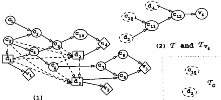
This section illustrates evaliD by using the ID in Fig­ ure 3, which is borrowed from Jensen et al (1994). Arcs into decision nodes are dashed for readability.

Denote the ID by N. Since it contains decision node, evaliD enters the while-loop. In the while-loop, Step l(a) finds that d4 is the tail decision node and Step l ( b ) constructs that reduced tail l=redTail(N, d4). To get a clear picture of I, note that the down­ stream set X 2 is { d4, cu, c12, v 4 } . Since no parents of d2 have parents in X2, 7fd4,2=0. Among the par­ ents of d4, only c10 and d4 are parents to nodes in 1fd4,2UX2\{d4}=X2\{d4}, hence c10 and d2 are the all the relevant parents of d4· In other words, 1fd4,r={cw, d2}. Consequently, I consists of nodes c10, d2, d4, cu, c12, and V4 and is as shown in Figure 4 (2), where v4 have been converted into a random node by Cooper's transformation.

Step l ( c ) calculates the evaluation functional e,-(1fd4,r, d4)· ·In the process, the BNs lc and /v4 are obtained from I by pruning nodes outside an(1fd4,r) and an(1fd4,rU{d4, v4}) respectively. Since an(1fd4,r )=1fd4,r={ c1o, d2}, lc consists of two nodes c1o and d2. They are isolated from each other and both have uniform distributions. Since an(7rd4,rU{v4}) con­ tains all nodes in the tail, fv4 is the same as T The

d4.

subroutine BNinf is called to compute the following probabilities:

Thereafter, the evaluation functional is obtained by

Step 1 ( d ) finds an optimal decision rule for d4 via 84(cw,d2) = arg maxd4eT(cw,d2,d4).

Step 1 (e ) calls augBody to construct the augmented body of N w.r.t d4, which is shown in Figure 4 (1). The utility function of the new value node U4 is given by fu4 (cw, d2) = maxd4eT(cw, d2, d4). Since no nodes in 1fd4,r have parents in X2, Step 1(f) is skipped.

We stop here due to space limit. Interested readers are referred to a longer version of the paper for the remaining steps.

6 Comparisons with previous methods

Both evaliD and the Shachter-Peot algorithm reduce ID evaluation into BN inference problems, which can be solved using arbitrary BN inference algorithms. This section shows that the probabilistic inference problems induced by evaliD are easier to solve than those induced by the Shachter-Peot algorithm.

Among all previous algorithms, Shenoy's fusion algo­ rithm ( Shenoy 1992) and the algorithms by Ndiliki­ likesha (1994) and Jensen et al (1994) are the most efficient. Those three algorithms are basically equiva­ lent in the sense that they all carry out essentially the same numerical computations. They are direct eval­ uation algorithms in the sense that they evaluate IDs directly without the reduction to BN inference prob­ lems. An method that reduces ID evaluation into BN inference problems would be unattractive if it is less ef­ ficient than those direct evaluation algorithms no mat­ ter what BN inference algorithm is used. We will show that this is not the case for evaliD by comparing it with Shenoy's fusion algorithm.

Non-numerical computations in evaliD include the identification of tail decision nodes, the construction of reduced tails and bodies, and pruning of nodes in a reduced tail that are irrelevant to particular BN in­ ference problems . They are negligible compared to numerical computations. We will hence focus the com­ parisons on numerical computations.

6.1 Comparisons with Shachter and Peot's algorithm

The Shachter-Peot algorithm applies only when there is one value node. Let N be an ID with one value node. Assume that there are no barren random nodes, i.e. random nodes that have no children3.

Let N' be the BN defined in Section 2. In the Shachter-Peot algorithm, the BN inference problem pN,(1fd,dlv=1) needs to be solved in order to obtain an optimal decision rule for the tail decision node d. Let T be the reduced tail of N w.r.t d. In evaliD, we need to solve two BN inference problems, namely PT(1fd,r) and PT(1fd,r,d,v=1).

The inference problem PN' (1fd, dlv=1) is more difficult to solve than PT(1fd,r) and PT(1fd,n d, v=1) than for two reasons. First, it involves more variables. Due to the no-forgetting constraint, all other decision nodes and their parents must be parents of d, i.e. in 1fd· However, as we have seen in the example of the pre­ vious section, many of the parents of d are irrelevant to d. The set 1r d,r usually contains much less variables than 1fd· Second, N' usually consists of many more nodes than the reduced tail T. Moreover, since N has no barren random nodes, no nodes in N' can be pruned when computing PN' (1fd, dlv=1), while T can be further reduced to Tc when computing PT(1fd,r) and Tv when computing PT(1fd,r, d, v=1).

In evaliD, nodes in the downstream set X2 are pruned after an optimal decision rule for d has been ob­ tained. In other words, those nodes do no participate in the computations for other decision nodes. How­ ever, no nodes are pruned in the Shachter-Peot algo­ rithm. Computations for each decision node involve all nodes inN.

6.2 Comparisons with Shenoy's fusion algorithm

This subsection first introduces a variation of evaliD, called evaliD1, that performs essentially the same

3 Barren random nodes, if exist, can be pruned at a pre­ processing step (Shachter 1986).

numerical computations as Shenoy's fusion algorithm and then compares evaliD with eval!D1.

6.2.1 A variation of evaliD

We will refer to non-negative functions of a set of vari­ ables simply as factors. Conditional probabilities and utility functions are all factors. Let p be an order­ ing of the nodes in X2\V2U{d}. In stead of evalFun, evaliD1 uses the following procedure to compute the evaluation functional of the reduced tail T and the marginal probability Pr( 1r d,r).

Procedure evalFun1(T, d)

1. Let F be the list of utility functions of value nodes in V2 and let P be the list of conditional probabilities of nodes in Xz\VzU{d}.
2. While p=/:-0, remove the first node x from p and call fuse(P,F,x).
3. Multiply all factor in P (the product is Pr(7rd,n d).)
4. Sum all factors in F (the result is er(7rd,n d)).
5. Return er(7rd,r,d) and 'L.d Pr(7rd,r,d).

The subroutine fuse is given as follows:

Procedure fuse(P,F,x)

1. Remove from P all the factors P1, ... , Pk that involve x. If such factors exist, add the new factor p = 'L- x TI � =l Pi to P.
2. Remove from F all the factors h, . . . , ft that involve x. If such factors exist, add the new factor 'L.x [ 'L. � =l fi](IJ� =l Pi]/p to F.

Let N be a value network and p be an ordering of the random nodes. Instead of expVal, eval!D1 uses the following procedure to compute the expected value of N.

Procedure expVal1(N):

1. Let F be the list of utility functions of value nodes in N and let P be the list of conditional probabilities of random nodes inN.
2. While p=/:-0, remove the first node x from p and call fuse(P,F,x).
3. Return the sum all factors in F (which is the expected value of N).

Shenoy's fusion algorithm requires an ordering, say p8, of all the random and decision nodes. If the or­ derings in evalFun1 and expVal1 conforms to Ps in the sense that relative orders of nodes are the same, than evaliD1 carries out essentially the same numer­ ical computations as Shenoy's fusion algorithm (see Shenoy 1992).

6.2.2 Comparisons

We now set out to compare evaliD1 and eval!D. Sup­ pose evaliD employs the VE (variable elimination) al­ gorithm 4 for probabilistic inference. Let A be a sub­ set of nodes in a BN M and let p be an ordering of nodes outside A. VE computes the marginal probabil­ ity PM(A) as follows:

Procedure BNinf-VE(M, A):

1. Let P be the list of conditional probabil­ ities in M .
2. While p=/:-0, remove the first node x from p and remove from P all the factors h, ... , fk that involve x. If such factors exist, add the new factor 'L- x TI � =l fi to the list P.
3. Multiply all factors in P and return the result (which is PM(A)).

Consider computing P�c (7rd,r) and P7, (1rd,r, d, v=1 ) using BNinf-VE. If the ordering in BNinf-VE conforms to the ordering in evalFun1, BNinf performs no more numerical computations than evalFun1(T, d). There­ fore, the amount of numerical computations carried out by evalFun(T, d) is at most 1 +m times that car­ ried by evalFun1(T, d), where m is the number of value nodes in T. Similarly, for any value network N, the amount of numerical computations carried out by expVal(N) is at most m times that carried by expVal1(N), where m is the number of value nodes inN.

We argue that evalFun(T, d) is usually more efficient that evalFun1(T, d), especially when T is large. De­ fine the size of a factor to be the number of vari­ ables involved in the factor. It is well understood in the BN literature that the complexities of BNinf and evalFun1 is largely determined by the sizes of the largest factors encountered; they are exponential in the largest factors sizes. The BNs Tc and each Tv are subnetworks ofT. When T is large, the differences between T and Tc or Tv are usually also large. In

4The idea behind VE is implicit in many papers (e.g. Shenoy 1992). It was first made explicit in Zhang and Poole (1994) and extended to exploit independence of causal in­ fluence by Zhang and Poole (1996).

such a case, the maximum factor sizes encountered by BNinf are smaller than those encountered by evalFun1 and hence the amount of time BNinf-VE spends in computing Pr;, (1T'd,r) or Pr;,(7rd , nd,v=1) is much less than that evalFun1(T, d) takes. Consequently, evalFun(T, d) takes less time than evalFun1(T, d).

A second reason for evalFun(T, d) being more efficient than evalFun1(T, d) is the fact that the former does not perform numerical divisions until the last step, while the latter might divide factors when fusing each node.

Similarly, expVal is usually more efficient than expVal. Hence evaliD is usually more efficient than evaliD1 and therefore more efficient than Shenoy's fu­ sion algorithm.

We would like to emphasize that arbitrary BN infer­ ence algorithms can be used in evaliD, while this is not the case in Shenoy's fusion algorithm and all the direct evaluation algorithms for that matter. This is a big advantage (see discussions in the next section).

7 Conclusions

This paper is about reducing ID evaluation into BN inference problems. Such an exercise is interesting be­ cause it allows the use of arbitrary BN inference algo­ rithms in evaluating IDs. Two reduction methods have been proposed previously (Cooper 1988 and Shachter and Peot 1994). A new method is presented in this paper. The BN inference problems induced by the new method are easier to solve than those induced by earlier methods.

When coupled with the VE algorithm, the perfor­ mance of the new method is, in the worst case, within a small constant factor of that of the most efficient pre­ vious algorithms, which evaluate ID directly without the reduction into BN inference problems. We have argued that the combination of the new method and VE is usually more efficient in large IDs.

The fact that it allows arbitrary BN inference algo­ rithms is big advantage of the new method. From a system development point of view, the method enables one to easily add ID evaluation capabilities to any BN inference packages. From the efficiency point of view, speeding up inference in BNs has been and still is an active research area. There are algorithms that ex­ ploit independence of causal influence (e.g. Zhang and Poole 1996) and that exploit special structures in the conditional probability tables. The new method facil­ itates ready incorporation of those algorithms, as well as future advances in BN inference, in ID evaluation. We are not aware of any approximate algorithms for IDs, while there is a rich collection of approximate and simulation algorithms for BNs. The new method also opens up the possibility of approximate algorithms for ID, which might be necessary in order to solve large decision problems.

References

• [I) G. F. Cooper (1988), A method for using belief networks as influence diagrams, in Proceedings of the Fourth Workshop on Uncertainty in Artificial Intelligence, pp. 55-63.
• [2) R. A. Howard, and J. E. Matheson (1984), In­ fluence Diagrams, in The Principles and Applica­ tions of Decision Analysis, Vol. II, R. A. Howard and J. E. Matheson (eds.). Strategic Decisions Group, Menlo Park, California, USA.
• [3) F. Jensen, F. V. Jensen, and S. L. Dittmer (1994), From influence diagrams to junction trees, Pro­ ceedings of the Tenth Conference on Uncertainty in Artificial Intelligence, pp. 367-373.
• P. Ndilikilikesha (1994), Potential influence di­ agrams, International Journal of Approximate Reasoning, 11, pp. 251-285.
• [5) J. Pearl (1988), Probabilistic Reasoning in Intel­ ligence Systems: Networks of Plausible Inference, Morgan Kaufmann Publishers, Los Altos, CA.
• R. Shachter (1986), Evaluating Influence Dia­ grams, Operations Research, 34, pp. 871-882.
• [7) R. Shachter (1988), Probabilistic Inference and Influence Diagrams, Operations Research, 36, pp. 589-605.
• [8) Shachter and Peot (1992), Decision making us­ ing probabilistic inference methods, in Proc. of 8th Conference on Uncertainty in Artificial Intel­ ligence, pp. 276-283.
• [9) P. P. Shenoy (1992), Valuation-based systems for Bayesian decision analysis, Operations Research, 40(3), pp. 463-484.
• [10) J. A. Tatman and R. Shachter (1990), Dynamic programming and influence diagrams, IEEE Transactions on Systems, Man, and Cybernetics, Vol. 20, pp. 265-279.
• [11) N. L. Zhang and D. Poole (1996), Exploiting causal independence in Bayesian network infer­ ence, Journal of Artificial Intelligence Research, 5, pp. 301-328.