Probabilistic Models for Agents' Beliefs and Decisions

Brian Milch

Computer Science Department Stanford University Stanford, CA 94305-9010 [email protected]. edu

Abstract

Many applications of intelligent systems require reasoning about the mental states of agents in the domain. We may want to reason about an agent's beliefs, including beliefs about other agents; we may also want to reason about an agent's preferences, and how his beliefs and pref­ erences relate to his behavior. We define a prob­ abilistic epistemic logic (PEL) in which belief statements are given a formal semantics, and provide an algorithm for asserting and query­ ing PEL formulas in Bayesian networks. We then show how to reason about an agent's be­ havior by modeling his decision process as an in­ fluence diagram and assuming that he behaves rationally. PEL can then be used for reasoning from an agent's observed actions to conclusions about other aspects of the domain, including un­ observed domain variables and the agent's men­ tal states.

1 Introduction

When an intelligent system interacts with other agents, it frequently needs to reason about these agents' beliefs and decision-making processes. Exam­ ples of systems that must perform this kind of reason­ ing ( at least implicitly ) include automated e-commerce agents, natural language dialogue systems, intelligent user interfaces, and expert systems for such domains as international relations. A central problem in many domains is predicting what other agents will do in the future. Since an agent's decisions are based on its be­ liefs and preferences, reasoning about mental states is essential to making such predictions. An equally important task is making inferences about the state of the world based on another agent's beliefs ( possibly re­ vealed through communication ) and decisions. Since other agents often observe variables that are hidden from our intelligent system, their beliefs and decisions may provide information about the world that the sys­ tem cannot obtain by other means.

Daphne Koller

Computer Science Department Stanford University Stanford, CA 94305-9010 koller@cs. stanford. edu

Suppose, for example, that we are developing a sys­ tem to help analysts and policymakers reason about international crises. In one example, based loosely on a scenario presented in [3], Iraq purchases weapons­ grade anthrax ( a deadly bacterium ) and begins to de­ velop a missile capable of delivering anthrax to targets in the Middle East. There is a vaccine against anthrax which the United States is currently administering to its troops, but for ethical reasons the U.S. has not done controlled studies of the vaccine's effectiveness. Iraq, on the other hand, may have performed such tests. Iraq's purpose in attempting to develop an anthrax­ equipped missile is to strike U.S. Air Force personnel in Turkey or Saudi Arabia, inflicting as many casual­ ties as possible. However, if Iraq works on developing the missile, it must use an old weapons plant that is prone to fire; a fire at the plant would be visible to U.S. satellites. We would like our intelligent system to be able to answer questions like, "If we observe that Iraq has purchased anthrax, what is the probability that the vaccine is effective?", and "Does Iraq believe ( e.g., with probability at least 0.3) that if they begin developing an anthrax-carrying missile, the U.S. will realize ( e.g., believe with probability at least 0.9) that they have acquired anthrax?".

Efforts to formalize reasoning about beliefs date back to Hintikka's work on epistemic logic [6]. The classical form of epistemic logic does not allow us to quantify an agent's uncertainty about a formula; we can only say that an agent knows <p or does not know <p. Prob­ abilistic logics of knowledge and belief [4, 16] remove this limitation. However, evaluating the probability that an agent a assigns to a formula <p in a model of one of these logics requires evaluating <p at every state that a considers possible. As the number of states is exponential in the number of domain variables, this process is computationally intractable.

One of the main contributions of this paper is the introduction of a probabilistic epistemic logic (PEL) that uses Bayesian networks ( BNs ) [12] as a compact

representation for the agents' beliefs. This framework allows us to perform probabilistic epistemic inference without enumerating an exponential number of states. Our approach is based on the common prior as­ sumption common in economics [1]. It states that the agents have a common prior probability distribu­ tion over outcomes and their beliefs differ only because they have different observations; this assumption al­ lows us to use a single BN for representing all the agents' beliefs. We describe an implemented algorithm for adding nodes to this BN so that it can be used to evaluate arbitrary PEL formulas.

In most domains, agents do not just passively observe the world and form beliefs; they also make decisions and act. In many existing probabilistic reasoning sys­ tems (e.g., [2, 13, 7]), a human expert defines the con­ ditional probability distributions (CPDs) that describe how likely an agent is to take each possible action, given an instantiation of the variables relevant to the agent's decision process. But this technique relies on a human's understanding of how agents make deci­ sions, and it may be difficult for a human to perform such analysis for a complex model. If we assume an agent acts rationally, the intelligent system can use de­ cision theory to derive the CPDs for the agent's actions automatically. This problem involves subtle strategic (game-theoretic) reasoning when multiple agents are acting and have uncertainty about each other's ac­ tions [5]. In this paper we restrict attention to the case where only one agent acts. We model the agent's decision process using an influence diagram (ID) [8], then convert this influence diagram into a Bayesian network. This extension allows us to use PEL in or­ der to reason about the decision-maker's likely course of action, and (more interestingly) to use his actions to reach conclusions about unobserved aspects of the world. We can also extend the framework to reach con­ clusions about the decision-maker's preferences, which may not be common knowledge.

2 A Probabilistic Epistemic Logic

Our probabilistic epistemic logic (PEL) is essentially a special case of the logic of knowledge and belief defined by Fagin and Halpern [4] (FH hereafter). In PEL, we assume that agents have a common prior probability distribution over states of the world, and an agent's local probability distribution at state s is equal to this global distribution conditioned on the set of states the agent considers possible at s. These assumptions are not uncontroversial, but we will defer a discussion of the alternatives until Section 6.

The language of PEL is parameterized by a set <I> of random variable symbols, each with an associated do- main; a set A of agents; and a number Na of observa­ tion stages for each agent a E A. At each of an agent's observation stages, there is a certain set of variables whose values the agent has observed. In this paper, we will make the perfect recall assumption: agents do not forget observations they have made. The values of the variables themselves do not change from stage to stage (if we want to model an aspect of the world that changes over time, we must create separate variables for separate times).

Given these parameters, the language of PEL consists of the following:

• atomic formulas of the form X= v, where X E <I> and v E dom(X) (the domain of X). Note that dom(X) need not be {true , false}; it may be any non-empty finite set.
• formulas of the form ''P and cp V 'if;, where cp and 'if; are PEL formulas; we use cp/\'1/; as an abbreviation for · ( ''P V ·'1/J).
• formulas of the form BelCond�.: ( cp I 'if;), where a E A, i E { 1 , ... , Na}, cp and 'if; are PEL for­ mulas, and r is a probability in [0, 1].

Our atomic formulas play the same role as propositions in the FH logic. The modal formula BelCond�,: (cp I 'if;) should be read as, "according to agent a in stage i, the conditional probability of cp given 'if; is at least r". The unconditional belief operator Bel�,: (cp) is an abbreviation for BelCond�: (cp I true). We will provide formal semantics for the�e statements after defining a model theory for PEL. Note that the ability to express conditional belief statements is not included in the FH logic, although their belief statements are more expres­ sive than ours in allowing probabilities to be related by arbitrary linear inequalities.

Definition 1 A model M of the PEL language having random variables <I>, agents A and observation process lengths {Na}aEA is a tuple (S, 1r, K, P), where:

• S is a set of possible states of the world;
• 1r is a value function mapping each random vari­ able symbol X E <I> to a discrete random variable X M (a function from S to dom(X));
• K maps each pair in { ( a, i) E A x z+ : i � Na} to an accessibility relation Ka,i which is an equiv­ alence relation on S;
• P is a probability distribution over S.

Thus, a PEL model specifies a set of states and maps each random variable symbol to a random variable de­ fined on those states. In the rest of the paper, we will often refer to a random variable X M simply as X; it should be clear from context whether a random vari­ able or a random variable symbol is intended. The

accessibility relation Ka,i holds between worlds that are indistinguishable to agent a at stage i. In other words, at stage i, if s and s' are in the same accessibil­ ity equivalence class, agent a has no information that allows him to distinguish between world s and world s'. We will use the notation Ka,i(s) to refer to the set of states s' E S such that Ka,i(s, s'). With this semantics, the perfect recall assumption is formalized as a requirement that if -Ka,i(s, s'), then for all j > i, we also have that -.Ka,j(s, s').

Pis the agents' common prior probability distribution over the set of states S. For each agent a, stage i, and state s, we can derive a local distribution Pa , i,s over the states accessible from s. This local distribution is the subjective probability that the agent assigns to each accessible state.

Definition 2 Consider any a E A, i E {1, ... , Na}, and s E S. Then for each state s' E Ka,i ( s) , we define: Pa,i ,s (s ') = P( s' I Ka,i(s)).

Note that an agent a's subjective probability distri­ bution varies from state to state. Thus, other agents' uncertainty about the state of the world can lead to uncertainty about a's beliefs. For example, in some states Iraq believes the anthrax vaccine to be effec­ tive, and in other states it does not; the U.S. may not be able to distinguish these two kinds of states.

The semantics of PEL will be familiar to readers with background in modal logic. We introduce a satisfac­ tion relation F=, such that ( M, s) F= r.p means the for­ mula r.p is satisfied at world s in model M. We also define an inverse relation [ r.p ] M = { s E S : s F= r.p}.

Definition 3 ( M, s) F= r.p if one of the following holds:

• r.p is an atomic formula X = v and X ( s) = v.
• r.p = -.'lj; and ( M, s) .lt 1/J.
• r.p = 'ljJ V x, and ( M , s) F= 'ljJ or ( M, s) F= X·
• r.p = BelCond�,: ( 1/J I x)' Pa,i,s ([x]M) =10, and Pa,i, s ( ['lf;]M I [X]M) � r.

Note that if there are no states accessible from s that satisfy x, then BelConda,i is defined to be false.

This definition of satisfaction allows us to evaluate a PEL formula at any states in a given model M. We can then use the prior probability distribution P to find the total probability of states that satisfy a for­ mula r.p. If we do this evaluation directly in the PEL model, we need to evaluate r.p at each of lSI states, and the size of the state space can be quite large - typ­ ically exponential in the number of variables. In the next section, we present a representation for PEL mod­ els based on Bayesian networks, and an algorithm that uses the independence assumptions encoded in the BN

to find the probabilities of PEL formulas efficiently.

Thus, we are proposing an efficient model-checking procedure for PEL formulas. We could also provide a proof system for PEL; in fact, Fagin and Halpern pro­ vide a complete axiomatization for their logic. How­ ever, it is reasonable to assume that an intelligent agent will have a complete model representing its own belief state, and it is often more efficient to assert and query formulas in a model than to attempt to derive formulas from a knowledge base (which would need to be quite large to completely define the agent's beliefs).

3 Representing a PEL model as a BN

Bayesian networks provide a compact representation of a complex probability space. We can augment Bayesian networks to provide a compact representa­ tion of a certain class of PEL models. The basic idea is as follows. We define a PEL model M over the set of random variables <I> using a BN B that has a node for each X E 1r(<I>). We define S to be the set of all possible assignments x to the variables in 1r( <I>). The distribution defined by B specifies the distribution P over S.

To define the accessibility relation Ka,i in this frame­ work, we place the restriction that an agent's obser­ vations always correspond to some set of random vari­ ables:

Observation Set Assumption: For every a E A and i E {1, ... , Na}, there is an observation set Oa,i C 1r( <I>) such that:

Given this assumption, the perfect recall assumption is equivalent to the requirement that if j > i, then Oa,i � Oa,j·

Definition 4 Let M = (S, 1r, K, P) be a PEL model; let B be a EN defining a joint distribution Pr and let Oa,i be observation sets consisting of random variables appearing in B. We say that M and ( B, {Oa,i}) are equivalent if:

• for every X E <I>, X is in B;
• for any instantiation x of 1r(<I>), P(x) = Pr ( x ) ;
• for each agent a and stage i, Ka,i is related to Oa,i according to the Observation Set assumption.

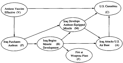
We can now use this framework to model the sce­ nario described in the introduction. The equiva­ lent Bayesian network is shown in Figure 1. Let i stand for Iraq and u stand for the United States. We assume that Iraq has a six-stage observation pro­ cess: Oi,l = {V}; Oi,2 = {V, P}; Oi,3 = {V, P, B};

Before it decides whether to attack the U.S. air base, is Iraq quite sure that U.S. casualties will be either high or medium? We can answer this question by evaluat­ ing the formula B el ( � · 8 ((C =high) V (C =medium)). A more complex q�ery is "Does Iraq believe with probability at least 0.3 that if they begin devel­ oping an anthrax-carrying missile, the U.S. will believe with probability at least 0.9 that they have acquired anthrax?". If we fill in the stages of the observation processes that are im­ plicit in this question, we get the PEL formula BelCond f g·3 ( Bel�.�·9 (P = true) I B = true ) .

The Observation Set Assumption implies that it is common knowledge what variables agent a has ob­ served at stage i. In many cases, this assumption is unrealistic; in our example, the U.S. might be un­ certain whether Iraq observed the effectiveness of the anthrax vaccine at stage 1. As we show, we can han­ dle such situations without modifying PEL. We simply add a new node Observes;,1 (V) to the BN of Figure 1. This node is true if Iraq has observed V at stage 1, and false otherwise; it can have as parents any nodes that are not descendents of V. We also add a node ObservedValue;,1 (V) that has V and Observes;,1 (V) as parents. Its domain is dom( V) U {unknown}. It takes the value unknown if Observes;,1 (V) is false, but has the same value as V if Observes;,1 (V) is true. We let 0;,1 contain Observes;,1 (V) and ObservedValue;,1 (V), but not V itself.

Under this construction, it is common knowledge that Iraq knows at stage 1 whether it has observed V at stage 1, and knows what value it has observed. However, since the value of Observes;,1 (V) is not common knowledge, the U.S. may not know whether ObservedValue;,1 (V) has the uninformative unknown value, or is a copy of V. We have defined this con- struction process with an example, but it is clearly general enough to model uncertainty about whether any variable X is in any observation set Oa,i· The modified BN and observation sets now define a PEL model over a richer set of states than simply the pos­ sible instantiations of 1r( <fl).

4 Evaluating PEL Formulas in a BN

This framework allows us to represent a PEL model compactly, but how do we answer queries such as the ones shown above? We can use an equivalent BN B to find the probability P(X = v) of any atomic formula, simply by finding Pr(X = v). We want to extend B so that it allows us to compute the probability of an arbitrary PEL formula cp. To this end, we first define an indicator variable 'TJ [cp] which is true if M, s F= cp and false otherwise. We then extend the BN to include not only the random variables 1r( <fl), but also indicator variables for some set � of formulas that we may assert or query. Since both 1r( <fl) and all such indicator variables are defined on S, the distribution P over S defines a joint distribution for 1r(<fl)Ury [�]. Our goal in constructing the augmented BN is to ensure that it defines the same joint distribution.

Definition 5 Let M = (S, 1r, K, P) be a PEL model; let B be an augmented BN defining a joint distribution Pr and let Oa,i be observation sets. Let � be a set of PEL formulas. Then M and (B, {Oa,i}) are �­ equivalent if M and B are equivalent and:

• for every cp E �' TJ [cp] is in B;
• for any instantiation x of (1r(<fl) U TJ [�]), P(x) = Pr(x).

We now present an algorithm that, given a BN that is equivalent to a PEL model M, adds indicator vari­ ables to create an augmented BN that is �-equivalent to M, for an arbitrary set of formulas �. The cen­ tral function of our algorithm is CreateNode(B, cp), which takes as arguments a BN l3 and a PEL formula cp. Its purpose is to create an indicator node for cp, store it in a global table, and give it the proper condi­ tional distribution given the other variables in B.

If there is already a node 'TJ (cp] in the table, CreateN ode returns immediately. If cp is an atomic formula X = v, then the function creates a node 1J (cp] whose sole parent is X. It defines the CPD of TJ [cp] such that 1J (cp] = true (with probability 1) if X = v, and TJ (cp] =false otherwise.

If cp = -.'lj.J, the function calls CreateNode(B, 'lj.J). Then it creates a node 'TJ (cp] with one parent, TJ ('lj.J]. It defines the CPD of 1J (cp] like a NOT gate: TJ (cp] = true iff TJ ('lj.J] = false. If cp = 'ljJ V x, the function calls

CreateNode(B,1P) and CreateNode(B,x). Then it creates a node TJ [<p] with two parents, TJ [1P] and TJ [x]. In this case, the CPD for TJ (<p] is like an OR gate: TJ (<p] = true iff TJ [1P] = true or TJ [x] = true.

The interesting case is where <p = BelCond�: (1P I x). As usual, the function begins by' calling CreateNode(B, 1P) and CreateNode(B, x). Now, recall that Oa,i is the set of variables whose values agent a has observed at stage i. Clearly, whether the agent assigns probability at least r to 1P given x depends on what the agent has observed. However, it may be that not all the observations are relevant; some of the variables in Oa,i may be d-separated from TJ [1P] given the other observations and TJ [x]. Using an algorithm such as that of (14], CreateNode determines the minimal subset Rei C Oa,i of relevant observations such that Oa,i -Rei is d-separated from TJ [1P] given Rei U {TJ [x]}. It then creates a node TJ (<p] with the elements of Rei as parents. Next, CreateN ode sets TJ [x] = true as evidence, and uses a BN inference algorithm (e.g., (10]) to obtain a joint distribution over TJ [1P] and Rei. For each instantiation rei of Rei, the function uses the joint distribution to calculate Pr(ry [1P] I (rei; TJ [x] = true)). We then set the CPD P(ry (<p] I rei) to give probability 1 to true if Pr( 1P I (rei; TJ [x] = true)) � r and probability 1 to false otherwise.

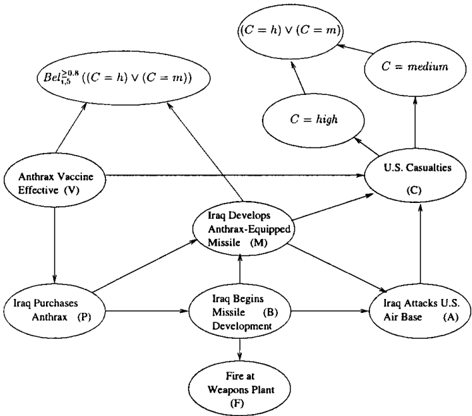
As an example of how this algorithm works, consider the formula we discussed earlier involving Iraq's beliefs about U.S. casualties:

Calling CreateNode on this formula results in a re­ cursive call to create a node for ((C = h) V (C = m ) , which in turn calls CreateNode for (C = h) and (C = m ) . There are five random variables in Iraq's observation set at stage 4, but it turns out that only two, V (vaccine effective) and M (missile developed), are relevant to ((C = h) V (C = m )) . To obtain the CPD for TJ [ <p ] , we perform BN inference to calculate Pr(ry [(C =h) V (C = m ) ] l rei) for each of the four in­ stantiations rei of { V , M}. In our parameterization of the model, it turns out that this probability is � 0.8 only when rei assigns false to V and true toM. So the CPD for TJ (<p] specifies true with probability 1 in this case, and false with probability 1 in the other three cases. The resulting BN is illustrated in Figure 2.

In proving the correctness of this algorithm, we will use the following lemma:

Lemma 1 Let M be a PEL model, a E A, i E {1, . . . , Na}, and s E S. Let Oa,i ,s be the instantia­ tion of Oa,i that s satisfies. Then for any formulas <p and 1P:

This lemma puts the criterion for satisfaction of BelCond�: (<p 11P) in a more convenient form. The proof, which we do not give here, uses the definition of Pa,i,s and the Observation Set assumption.

Proposition 1 (Correctness of CreateNode) Suppose an augmented BN B is D.-equivalent to a PEL model M. Then when CreateNode(B, <p) terminates, B is (6. U {<p})-equivalent toM.

Proof: We use structural induction on <p; the induc­ tive hypothesis is that Proposition 1 holds for all sub­ formulas of 1PThus, the recursive calls at the begin­ ning of CreateNode make it so B is f-equivalent to M, where r is 6. plus all the subformulas of <p. Then CreateNode(B, <p) adds TJ ( <p ] to B. Let Pr be the dis­ tribution defined by B before this addition, and Pr' be the distribution afterwards.

By the definition of f-equivalence, we know that for every instantiation x oh(<J>)Ury (f], P(x) = Pr(x). We must show that for every instantiation (x; (TJ [<p] = t)) of 1r(<J>) U TJ ( 6.] U {TJ ( <p ] } :

Let pa be the instantiation x limited to the par­ ents of the newly created node TJ [ <p ] . Then by the definition of conditional probability and the chain

rule for Bayes nets, equation (1) is equivalent to: P(ry [cp) = t I x) · P(x) = Pr'(ry [cp) = t I pa) · Pr'(x). CreateN ode only adds nodes as children of existing nodes, so the marginal distribution over existing nodes is not changed. Thus Pr' (x) = Pr(x). Along with the fact that P(x) = Pr(x), this allows us to reduce equa­ tion (1) to:

So what we must show is that the CPDs defined by CreateN ode are the correct CPDs for the indicator variables. The cases where cp is an atomic or Boolean formula are straightforward, so we move directly to the interesting case where cp = BelCond�,: ('lj; I x) .

In this case, CreateNode adds a node 'fJ [cp) with the relevant members of Oa,i as parents (to simplify the presentation, we will assume that all members of Oa,i are relevant). Suppose x assigns values Oa,i to Oa,i · Then what we have to prove is:

Consider any state s in which x holds. By Lemma 1 and the definition of satisfaction, 'fJ [cp) (s) = true if and only if: P (ry ['l/;) = true I Oa,i,s, 'f] [x] =true) 2': r. But 'ljJ and x are subformulas of cp, and Oa,i C II>, so by the assumption that B is r-equivalent toM:

This last probability value is exactly what CreateNode compares to r in constructing the CPD for 'fJ [cp). So the CPD is correct. ·

Once we have a BN that is Ll-equivalent to M we can assert any formula cp E Ll by setting 'f] [ cp ) = true as ev­ idence. To find the probability of any formula cp E � ' we simply query 'f] [cp) = true. For example, the for­ mula cp = Bel��-8 ((C =h) V (C = m )) that we dis­ cussed earlier has probability 0.16 in our model. How­ ever, if we assert V =false (i.e., the vaccine is ineffec­ tive), then Pr(cp) goes up to 0.8.

The number of BN queries required to make a BN �­ equivalent toM is linear in the number of BelCond for­ mulas, since CreateN ode is only called once for each subformula. The CreateNode function takes time exponential in the maximal number of relevant obser­ vations for the BelGond subformulas, as we need to compute the probability Pr(ry ['1/J) I (rei; 'f] [x] = true)) for every instantiation rei of Rei. Most naively, we simply run BN inference for each rei separately. In cer­ tain cases, we can get improved performance by run­ ning a single query Pr(ry ['l/;), Rei I 'f] [X] = true) and then renormalizing appropriately; this approach can

allow us to exploit the dynamic programming of BN inference algorithms. We note that the newly added nodes also add complexity to the BN, and can make the inference cost grow in later parts of the computa­ tion (e.g., by increasing the size of cliques).

5 Reasoning about Decisions

So far, we have assumed that we have a probability distribution over all variables in the system. In prac­ tice, however, we have agents who make decisions in accordance with their beliefs and preferences. In our example, P, B and A are actually decisions made by Iraq. Our construction took these to be random vari­ ables, each with a CPD representing a distribution over Iraq's decision. If these CPDs are reasonable, then our system will give reasonable answers; e.g., we will obtain a lower probability that the anthrax vac­ cine is effective if we observe that Iraq has purchased anthrax, since it would not be rational for Iraq to pur­ chase a bacterium for which the U.S. has an effective vaccine. We would like to extend our framework to in­ duce automatically the actions that agents will take at various decision points. As discussed in the introduc­ tion, this problem is quite complex when there are mul­ tiple decision makers with conflicting goals. We there­ fore focus on the case of a single decision maker. We note, however, that we can still have multiple agents reasoning about the decision maker and about each other's state of knowledge.

Assuming that agents act rationally, we can automate the construction of CPDs for decision nodes by mod­ eling the decision maker's decision process with an in­ fluence diagram, and solving the influence diagram to obtain CPDs for the decision nodes. Somewhat sur­ prisingly, the possibility of modeling other agents with influence diagrams has not been explored deeply in the

existing literature, although Nilsson and Jensen men­ tion it in passing [11 ] . Suryadi and Gmytrasiewicz [15] take an approach similar to ours in that they use an ID to model another agent's decision process. However, they discuss learning the structure and parameters of the ID from observations collected over a large set of similar decision situations. We assume that the ID is given, and concentrate on the inferences that can be made only from a few observations about the current situation.

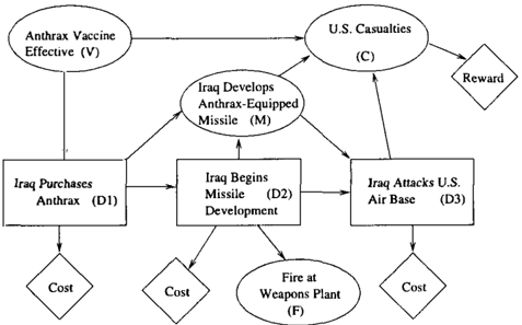
Figure 3 depicts an influence diagram for the scenario described in the introduction. An influence diagram is a directed acyclic graph with three kinds of nodes. Chance nodes, like nodes in a BN, correspond to ran­ dom variables; they are represented by ovals. Decision nodes, drawn as rectangles, correspond to variables that the decision-maker can control. Utility nodes, drawn as diamonds, correspond to components of the decision-maker's utility function.

The decision nodes of an ID are ordered D1, ... , Dn according to the order in which the decisions are made. The parents of D;, denoted Pa(D;), are those variables whose value the decision-maker knows when decision D; is made. Thus, when we are creating a PEL model and an ID for the same scenario, the decision-maker's observation stages correspond to his decision nodes, with Oa,i equal to Pa(Di). A utility node U; repre­ sents a deterministic function fi from instantiations of Pa( U;) to real numbers. The utility of an outcome is the sum of the individual utility functions k

Solving an influence diagram means deriving an opti­ mal policy, consisting of a decision rule for each deci­ sion node. A decision rule 6; for a node D; is a function from dom(Pa(D;)) to dom(D;). For each instantiation of Pa(D;), the decision rule gives the action that max­ imizes the decision-maker's expected utility, assuming it will act rationally in all future decisions. The stan­ dard algorithms for solving IDs utilize backwards in­ duction: the decision rules for the decision nodes are calculated in the reverse of their temporal order [9].

After we have the decision rules, we can easily trans­ form an influence diagram V into a Bayesian network B(V). We remove the utility nodes, and change the de­ cision nodes into chance nodes (ordinary BN nodes). If D; is a decision node, then for each instantiation pa of Pa(D;), we create a probability distribution that gives probability 1 to J;(pa), and probability 0 to all other elements of dom(D;). This distribution becomes the CPD for D; given pa.

We can use this system to make inferences about un­ observed world variables based on evidence of agents' actions. Suppose the parameters of the model V de­ picted in Figure 3 are such that the prior probability of the vaccine being effective is 0.8, but it is irrational for Iraq to purchase anthrax unless it has observed the vaccine to be ineffective. As above, we may need to add some additional nodes to V, such as Observed and ObservedValue nodes to model the U.S.'s uncertainty about whether Iraq observes V at stage 1. We then use the method described in this section to derive CPDs for Iraq's decision nodes, creating a BN B(V). The in­ fluence diagram defines the observation sets for Iraq; we will use the U.S. observation sets described in Sec­ tion 2. We can then use the algorithm of Section 4 to find the probabilities of arbitrary PEL formulas in the PEL model corresponding to B(V).

At stage 1, the U.S. assigns probability 0.8 to the vaccine being effective: all states satisfy Bel�,�-8 (V =true). At stage 2, however, the situation changes. It turns out that Bel�,�-8 (V = true) is true if and only if there is not a fire at the Iraqi bi­ ological weapons plant. A fire provides the U.S. with strong evidence that Iraq has begun developing an anthrax-carrying missile, which would not be ratio­ nal unless Iraq had purchased anthrax, which implies that Iraq has observed the anthrax vaccine to be in­ effective. So in this model, Pr(Bel��-8 (V =true)) = Pr(F = false). In a more comple� query, we could compute Pr(Bel��-8 (V = true) I V =false), i.e., the probability that the U.S. will believe the vaccine to be effective despite the fact that it is not. The answer to this query would depend on the prior probability about the vaccine's effectiveness, Iraq's decisions, and the chances of observing a fire.

The CPDs for decision nodes derived by solving an influence diagram become part of the common prior distribution in the resulting BN. However, these CPDs are derived using the decision-maker's utility function. Thus, in assuming that the decision-maker's decision rules are part of the common prior, we are implicitly assuming that the decision-maker's utility function is common knowledge. Like the assumption that obser­ vations are common knowledge, this is an assumption we would like to relax.

Just as we introduced Observes nodes to model un­ certainty about an agent's observations, we can in­ troduce preference nodes to model uncertainty about an agent's utility function. These preference nodes are parents of particular utility nodes, and modify the way the utility depends on other variables. They are also in all the decision-maker's observation sets, as­ suming he knows his own preferences. One might pro­ pose to use continuous-valued preference nodes that define a distribution over the decision-maker's util­ ity value. The problem with this approach is that these continuous-valued preference nodes must be par­ ents of every decision node, and standard ID solution

algorithms cannot handle continuous values in such a context. We therefore use discrete-valued prefer­ ence nodes, with the resulting coarse-grained prefer­ ence models. For example, we can introduce a node A representing Iraq's aversion to doing business with criminal biological weapons dealers, which is a parent of the cost node associated with D1. If A = high, then the cost is greater in magnitude than it would be if A = low. The preference node A is in the parent sets of all Iraq's decision nodes, but the U.S. will not be able to observe it directly.

6 Discussion and Future Work

This paper combines epistemic logic with Bayesian networks to create an integrated system for probabilis­ tic reasoning about agents' beliefs and decisions. Al­ though PEL is essentially a restricted version of the logic presented by Fagin and Halpern, we believe it is flexible enough to be useful in many practical applica­ tions. Furthermore, the simplicity of PEL allows us to define an algorithm for finding the probability of a for­ mula in a PEL model using a Bayesian network, rather than constructing the PEL model explicitly. We also show how to construct this Bayesian network from an influence diagram, rather than having a human fill in the CPDs for nodes that represent an agent's decisions.

Our approach is limited by the common prior assump­ tion, which implies that all differences between agent's beliefs are due to their having different observations. This assumption is common in economics, and has important ramifications [1]. It allows agents' beliefs to be arl;>itrarily diffenmt, as long as they have re­ ceived sufficiently different observations. But it may be impractical to represent in a BN all the different observations that have caused agents' beliefs to di­ verge. An alternative is to explicitly represent un­ certainty about each agent's probability distribution. However, this approach introduces substantial com­ plications: Do we also model one agent's distribution about another agent's distribution? If so, do we model the infinite belief hierarchy? Therefore, the extension to this case is far from obvious. Another assumption that we would like to relax is that agents are perfect probabilistic reasoners and decision makers.

The other obvious limitation of the system described in this paper is that although it can reason about the beliefs of an arbitrary number of agents, it can only reason explicitly about one agent's decisions. If we wish to have the system automatically derive the CPDs for decisions made by multiple agents, the max­ imum expected utility solution concept is no longer appropriate, since the agents do not have probability distributions over each other's actions. We could uti- lize game-theoretic solution concepts [5] to find ratio­ nal strategies for the agents, and then substitute these strategies for the agents' CPDs as we did in Section 5; the rest of our results would still be applicable. How­ ever, the framework of multi-agent rationality is sub­ stantially more ambiguous than the single agent case, so that this approach does not define a unique answer. We hope to investigate this issue in future work.

Acknowledgments. We thank Yoav Shoham for use­ ful discussions and Uri Lerner and Lise Getoor for their work on the PHROG system. This work was supported by ONR contract N66001-97-C-8554 under DARPA's HPKB program.

References

1. R. J. Aumann. Agreeing to disagree. Annals of Statis­ tics, 4(6):1236-1239, 1976.
2. E. Charniak and R. P. Goldman. A Bayesian model of plan recognition. Artificial Intelligence, 64(1) :53-79, 1993.
3. P. Cohen, R. Schrag, E. Jones, A. Pease, A. Lin, B. Starr, D. Gunning, and M. Burke. The DARPA High Performance Knowledge Bases project. AI Mag­ azine, 19(4):25-49, 1998.
4. R. Fagin and J. Y. Halpern. Reasoning about knowl­ edge and probability. J. ACM, 41(2):340-367, 1994.
5. D. Fudenberg and J. Tirole. Game Theory. MIT Press, 1991.
6. J. Hintikka. Knowledge and Belief. Cornell University Press, Ithaca, New York, 1962.
7. E. Horvitz, J. Breese, D. Heckerman, D. Hovel, and K. Rommelse. The Lumiere project: Bayesian user modeling for inferring the goals and needs of software users. In Proc. UAI, pages 256-265, 1998.
8. R. A. Howard and J. E. Matheson. Influence dia­ grams. In Readings on the Principles and Applica­ tions of Decision Analysis, pages 721-762. Strategic Decisions Group, 1984.
9. F. Jensen, F. V. Jensen, and S. L. Dittmer. From influence diagrams to junction trees. In Proc. UAI, pages 367-373, 1994.
10. S. L. Lauritzen and D. J. Spiegelhalter. Local compu­ tations with probabilities on graphical structures and their application to expert systems. J. Royal Stat. Soc. B, 50(2):157-224, 1988.
11. D. Nilsson and F. V. Jensen. Probabilities of future decisions. In Proc. IPMU, 1998.
12. J. Pearl. Probabilistic Reasoning in Intelligent Sys­ tems: Networks of Plausible Inference. Morgan Kauf­ mann, San Mateo, California, 1988.
13. D. V. Pynadath and M. P. Wellman. Accounting for context in plan recognition, with application to traffic monitoring. In Proc. UAI, pages 472-481, 1995.
14. R. D. Shachter. Bayes-ball: The rational pastime. In Proc. UAI, pages 480-487, 1998.
15. D. Suryadi and P. J. Gmytrasiewicz. Learning models of other agents using influence diagrams. In J. Kay, editor, Proc. 7th Int'l Conf. on User Modeling, pages 223-232, 1999.
16. W. van der Hoek. Some considerations on the logic PFD: A logic combining modality and probability. J. Applied Non-Classical Logics, 7(3):287-307, 1997.