Properties of Bayesian Belief Network Learning Algorithms

Remco R. Bouckaert -PhD student Utrecht University Department of Computer Science P.O.Box 80.089 3508 TB Utrecht, The Netherlands remco@cs .ruu.nl

Abstract

In this paper the behavior of various be­ lief network learning algorithms is stud­ ied. Selecting belief networks with cer­ tain minimallity properties turns out to be NP-hard, which justifies the use of search heuristics. Search heuristics based on the Bayesian measure of Cooper and Her­ skovits and a minimum description length (MDL) measure are compared with re­ spect to their properties for both limit­ ing and finite database sizes. It is shown that the MDL measure has more desir­ able properties than the Bayesian mea­ sure. Experimental results suggest that for learning probabilities of belief net­ works smoothing is helpful.

Keywords: Bayesian belief networks, learning, Bayesian approach, minimum description length principle, K2.

1 Introduction

The framework of Bayesian belief networks offers a mathematically sound formalism for representing uncertainty in knowledge-based systems. Efficient algorithms are associated with the formalism for making inferences with knowledge represented in be­ lief networks, [Henrion, 1990; Lauritzen and Spiegel­ halter, 1988; Pearl, 1988]. In addition, the frame­ work has proved its practical worth over the last few years. However, constructing belief networks with the help of human experts is a time-consuming task. Since more and more large databases become available, automated learning algorithms can help shorten the build and test cycle of a belief network by suggesting an initial set-up. Therefore, learning belief networks from data is an important research issue.

In various fields of science, a lot of research ef­ fort has been spent on the design of methods for learning Bayesian belief networks from different per- spectives such as computer science, statistics, and philosophy. One of the most promising to date is a Bayesian method proposed by Cooper and Her­ skovits, [Cooper and Herskovits, 1992]. However, methods based on the minimum description length principle are rapidly gaining popularity, [Bouck­ aert, 1993; Lam and Bacchus, 1994; Suzuki, 1993; Wedelin, 1993]. In this paper, the properties of sev­ eral learning algorithms are investigated.

All these methods incorporate three elements; a quality measure for deciding which of a set of net­ work structures is best, a search heuristic for sug­ gesting a set of network structures to compare, and an estimation method for learning the probabilities in the network.

In the next section, we give a short introduction to terms and notations used in the remainder of this pa­ per. Section 3 is devoted to the properties of quality measures. In Section 4, we consider search heuris­ tics. In Section 5, we investigate learning proba­ bilities for a Bayesian belief network. To compare various learning algorithms, we performed some ex­ periments, the results of which are discussed in Sec­ tion 6. We conclude with some final considerations and directions for further research.

2 Preliminaries

A Bayesian belief network B over a set of variables U is a pair ( B s, B p). B s is called the network structure of B and takes the form of a directed acyclic graph with one node for each variable in U. For simplicity, we assume that the variables in U are discrete. B p is a set of conditional probability tables; for every vari­ able x; E U, Bp contains a conditional probability table with parameters P( x; l1ri) that enumerates the probabilities of all values of x; given all combinations of values of the variables in its parent-set 1r; in the network structure Bs. The distribution represented by such a network B is P(U) = l1x;EU P(x;l7r;), [Pearl, 1988].

In a network structure Bs, a trail is a path that does

not consider the direction of the arcs. A head-to­ head node in a trail is a node e such that the sequence x --1e +y is part of the trail. A trail between two nodes x and y is blocked by a set of nodes Z if at least one of the following two conditions hold:

• the trail contains a head-to-head node e such that e !f. Z and every descendant of e is not in Z;
• the trail contains a node e such that e E Z and e is not a head-to-head node in the trail.

In a network structure Bs, let X, Y and Z be sets of nodes. We say that X is d-separated from Y given Z if every trail between any node x E X and any node y E Y is blocked by Z.

For a joint probability distribution P over a set of variables U, we call X and Y conditionally inde­ pendent given Z, written I(X, Z, Y), if P(XY!Z) = P(X!Z)P(Y!Z) for all values of the variables in XYZ. I(X, Z, Y) is called an independency state­ ment.

A network structure Bs is an independency map or !-map of a distribution P if X and Y being d-separated by Z in Bs implies that I(X, Z, Y) holds in P; Bs is a minimal !-map of P if no arc can be removed from Bs without destroying its I­ mappedness. Bs is a perfect map or P-map of P if it is an I-map and I(X, Z, Y) holding in P implies that X andY are d-separated by Z in Bs.

In discussing the various algorithms, we assume that cases in the database occur independently and, there are no cases that have variables with missing values.

3 Quality Measures

The task of learning Bayesian belief networks is twofold; learning the network structure Bs and learning the set of probability tables Bp. The latter task will be addressed in a later section. Here, we investigate learning network structures.

For learning network structures, we use a quality measure. With such a measure a network struc­ ture that has a higher quality is preferred above a network structure with a lower quality. A heuris­ tic search procedure is performed to select a net­ work structure that has the highest quality among the considered network structures.

Cooper and Herskovits [Cooper and Herskovits, 1 992] have proposed a quality measure based on a Bayesian approach in which they assume that no probability table Bp is preferred for a given network structure before the database has been inspected.

Let U be a set of n discrete variables x;, where each x; can take one of r; different values V i 1 , ... , Vir;, i = {1, . .. ,n } r; 2:2. Let D be a database of N cases where each case specifies a value for each variable in U. Let Bs denote a network structure over the variables in U. For each Xi, let 1ri be the parent set of x; in Bs; let Wij denote the jth instantiation of 1ri relative to D, j == 1, ... q,, q; :2:1. Now let Nijk be the number of cases in D in which variable x; has the value Vik and 1r, is instantiated as w;i, and let N;j = 2:: � � 1 Nijk· Let P(Bs) be the probability of Bs prior to observation of the database. Then, the probability of Bs and the database D is,

For a proof, we refer to [Cooper and Herskovits, 1992]. In practical implementations, generally the logarithm1 of Equation (1) is taken; the result will be referred to as the Bayesian measure of the quality of a network structure.

Another measure for networks is the description length,

fi d L n L q· L r N ·· · N · · ne as . ' ' -�log � and k as t=l J=l k=l N N;1 L�=l ( r; -1) ITx;E,., Tj. It has been shown [Bouck­ aert, 1993] that (2) is approximately equal to the Bayesian measure except for error terms that are less than 0(1) with respect to N. Compared to the Bayesian measure, this measure has a more intuitive interpretation. When Formula (2) is interpreted as approximation of the Bayesian measure, the term log P(Bs) may seem superfluous since it is of the same order as the approximation errors. Still the term remains useful for incorporating prior informa­ tion. For example, prior information on the exis­ tence and direction of arcs can be incorporated in this term. The term -N · H(Bs,D) is -N times the entropy of a network structure Bs and database D. Generally, this term increases as arcs are added to a network structure. In the last term, k equals the number of independent probabilities that are needed to define all probability tables in Bp for Bs. The term -! k ·log N thus models the cost of estimating these k probabilities. Contrary to the entropy term, this term decreases when arcs are added to a network structure. When no prior information is available so P(Bs) is equal for all network structures Bs, this measure assigns high quality to network structures that fit the database with as few arcs as possible. Therefore, Equation (2) will be referred to as the minimum description length (MDL) measure for the quality of a network structure.

3.1 Properties of Quality Measures

This section will be devoted to the investigation of the behavior of the Bayesian and MDL measures.

1 All logarithms are to the base two.

We say that a network structure Bs obeys a total ordering < u on the variables U if for every arc Xi --+ X j in Bs xi <u xJ.

Theorem 3.1 Let Pn be a positive distribution over a set of variables U. Let D be a database with N cases generated by Pn where N approximates in­ finity. Let <u be a total ordering on U. Let Bs be the minimal !-map of Pn that obeys <u. Then, for any network structure Bs' Bs' i= Bs that obeys <u,

where M is either the Bayesian or the MDL mea­ sure.

A proof of this theorem can be found in [ Bouckaert, 1994]. The theorem states that for databases large enough, networks that are minimal Imaps that obey a particular ordering <u are overwhelmingly pre­ ferred over networks that are non-minimal I-maps. As a consequence, we have that if a P-map exists that obeys <u then this P-map will be overwhelm­ ingly preferred.

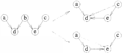
It is interesting to investigate the properties of the quality measures when no ordering on the vari­ ables is provided. However, minimal I-maps are not unique when no ordering needs to be obeyed. Uniqueness of optimal structures is a desirable prop­ erty since it helps deriving theoretical results and is important for deriving causal structure. Mini­ mal I-maps need not even be equivalent, that is, represent the same set of independency statements. Consider for example Figure 1; if the structure on the left is a P-map of a distribution P, then both other structures on the right are minimal I-maps of P marginalised over b. However, the upper struc­ ture represents I( a, 0, e) while the lower structure does not.

Also, the number of probabilities that need to be es­ timated for minimal I-maps need not be the same. This gives reason to distinguish between minimum and non-minimum structures. A minimum !-map Bs of a distribution Pis a minimal I-map of P such that in the belief network B = (Bs, Bp) the least number of probabilities need to be specified in order to define all probability tables Bp. Consider once more Figure 1 and let all variables be binary; then, for both I-maps twelve probabilities need to be spec­ ified, one for a one f o r c and eight and two ford and e (e and d) in the upper ( lower ) network structure. We have the following theorem for minimum I-maps.

Theorem 3.2 Let Pn be a distribution over a set of variables U. Let the prior distribution over all network structures over U be positive. Let D be a database with N cases generated by Pn where N ap­ proximates infinity. Let Bs be a minimum !-map of Pn. Then, for any non-minimal !-map Bs, of Pn we have that,

where M is either the Bayesian or the MDL mea­ sure.

The theorem suggests that for databases large enough, network structures that are minimum I­ maps are preferred over network structures that are non-minimum I-maps. Note that contrary to The­ orem 3.1 no positive distribution Pn is demanded. The theorem also suggests that if a P-map exists for a distribution then a P-map is preferred over non P-maps for large databases; this follows from the property that all P�maps require the same number of probabilities and every I-map that is not a P-map requires more probabilities. A proof of this property can be found in [ Bouckaert, 1994]. Note that also P-maps need not be unique; if a --+ b is a P-map then a+--b is also a P -ma p .

We are interested in properties of network structures that are selected when a quality measure is used. The following theorem gives some insight.

Theorem 3.3 Let D be a database with N cases over U, N :::: 10. Let Bs be a network structure over U, with at least one parent-set containing log N variables or more. If no prior information is avail­ able then, a network structure Bs' exists such that L(B5,,D) > L(B5,D).

Again a proof can be found in [ Bouckaert, 1994]. The theorem implies that search algorithms that use the MDL measure will not select network structures that contain parent-sets with more than log N par­ ents. A similar result would be expected for the Bayesian measure. However, consider a database Di recursively defined by

where the rows represent the individual cases and the columns the values of the variables; Dn is con­ structed from Dn-l by adding a column for an ex­ tra variable Xn filled with 1s. Further, two identical cases are added where xi = 0 (1 :s:; i :s:; n) and y = ( n+l ) mod 2. For example, Figure 2 shows how D1 is build from D1 up to D6.

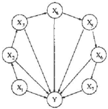
Figure 3 shows the network structure that scores highest with the Bayesian measure; all nodes Xi have

X 6

Figure 2: Example of databases D; up to D7.

X7	6	xs	X4	X3	x2	x,	y
0	0	0	0	0	0	0	0
0	0	0	0	0	0	0	0	Dr
1	0	0	0	0	0	0	1
1	0	0	0	0	0	0	1	DB
1	1	0	0	0	0	0	0
1	1	0	0	0	0	0	0	Ds
1	1	1	0	0	0	0	1
1	1	1	0	0	0	0	1	D4
1	1	1	1	0	0	0	0
1	1	1	1	0	0	0	0	D3
1	1	1	1	1	0	0	1
1	1	1	1	1	0	0	1	D2
1	1	1	1	1	1	0	0
1	1	1	1	1	1	1	1	D,

a node x,_1 in their parent-set while y has all nodes x,, ... , x7 in its parent-set. This network was found by brute force; the Bayesian measure was calculated for all 1.138.779.265 possible networks. Obviously, the parent-set of node y contains more than log(14) parents.

The same behavior arises for larger databases D1 j > 7. The Bayesian measure will prefer parent-sets 71'; of x; if knowledge of the values of 71'; gives information of the distribution of x; while the number of states of the parent-set q; is not too large.

Let us consider the parent-sets of the best structure for Dj according to the Bayesian measure. In D1, nodes x; (1 < i < j) will have x;-1 in their parent­ set because when x;_1 is 1, we find in the database that x; is 1. Furthermore, Xi+l may be in 71'; be­ cause when x;+1 is 0, we find in the database that Xi is 0. The only variable that gives more informa­ tion is y; Xi is a function of X;-1, XiH and y in the database. However, adding y to the parent-set of x; would increase qi relatively much while the in­ formation obtained only applies to four cases in the database. For Xj (x1) a similar argument holds, ex­ cept that x J+ 1 (x0) is non-existant and need not be considered.

What remains to be considered is node y. By an inductive argument, it can be shown that if 1l'y is x�.;, . . . ,xj 1 < k $ j then taking Xk-!, ... ,Xj for

7r y results in a better score. Further, any parent­ set of size s gives exact information for at most as much cases for y as Xj-s+l, . . . , Xj so these sets score worse. Therefore, the best scoring parent-set for y is x1, ... , x j in D j. So, we have that in a database with N cases, a network with parent-sets with N /2 variables can be assigned quality by the Bayesian measure.

So, while the asymptotic behavior of the Bayesian and MDL measure is the same, this is not the true for the practical case for which a finite database is available.

4 Search Algorithms

Recall that the purpose of an algorithm for learn­ ing network structure from data is to select a net­ work structure with highest quality according to a given quality measure. The number of different net­ work structures is more than exponential in the num­ ber of variables; for example, there are more than 4.2 x 101 8 network structures for 10 variables. The search space of possible structures for a learning al­ gorithm is very large. We will show that the problem of finding a structure with minimality properties are NP-hard.

Theorem 4.1 Let P be a given probability distribu­ tion over a set of variables U and let an oracle be available that reveals wether an independency state­ ment holds in P or not. Then, the problem of finding an !-map of P with a minimum number of arcs is NP-hard.

A proof can be found in [Bouckaert, 1994]. From the theorem we have that no efficient algorithm exists for constructing a network structure with a minimal number of arcs, not even when we know the distri­ bution that is to be represented. As a consequence we have that no minimum I-map can be found under the same conditions.

In [Cooper and Herskovits, 1992], Cooper and Her­ skovits proposed an algorithm, called K2. This al­ gorithm departs from a given ordering on the vari­ ables. For simplicity, it is assumed that no prior information on the network is available, so the prior probability distribution over the network structure is uniform and can be ignored in comparing network structures. The algorithm is a greedy heuristic. For each variable x;, the algorithm starts with an empty parent-set and tries to add variables to this set; a variable that is lower numbered than x; and maxi­ mally increases the quality is added to the parent-set 7!'; of x;. This process is repeated until adding such variables does not increase the quality anymore or the parent-set consists of all lower numbered vari­ ables.

In the algorithm, mi(7r;) represents the the con­ tribution of variable x; with parent-set 71'; to the

Algorithm K2 Let the variables be ordered XI, ... , Xn fori E {1, ... ,n} do {initialize} 7r; +- 0 foriE{2, ... ,n}do {main loop} repeat select y E {xi ... x;-d\7r; that maximizes g = m;(1r; U {y}) .6. +- gm;(7r;) if .6. > 0 then 7r; +7r; u {y} until .6. s; 0 or 7r; = {XI, .. . , Xi-1 }

measure used; we implicitly assume that we work with a database D, so D is omitted in the no­ tation. When the Bayesian measure is used, we h ( ) - l (IJq; (r;-1)! IJr' N ' ) d ave m; 7r; -og j=l (N,,+r,-11, k=I i j k · an when the MDL measure is used we have m;(7r;) = 2::]�1 E��� Nijk log �;, " -�q;(r; -1) log N. Note that in theory, the change of the measure given the complete network need be computed. However, all terms other than the ones mentioned cancel out.

The main drawback of K2 is that it makes use of an ordering of the variables. If no reasonable ordering is available, a random ordering may be chosen which may be optimized in a post-processing step.

A learning algorithm that does not require an order­ ing of variables was suggested by [Buntine, 1991a]. This algorithm also uses a greedy heuristic. As K2, it starts with empty parent-sets for each node. In each step, an arc is added that does not introduce a cycle in the network abd maximally increases the quality of the network. Arcs are added until further addition does not increase the quality of the network or no candidate arcs are left.

An efficient implementation called algorithm B is shown below; Pred; is the set of indices of the pre­ decessors of x; and Desc; is the set of indices of descendants of x; including i.

As the output of algorithm B need not be a minimal I-map, it is wise to have a post-processing step that optimizes the ordering of the variables as implied by the structure generated by algorithm B.

To conclude, we consider the complexity of algo­ rithms K2 and B in terms of computations of m;(7r;). Both algorithms will calculate m; ( 7r; ) at most O(n2 · u) times where u is an upper limit to the number of parents of a variable. Calculation of m;(7r;) takes at most O(N ·r) calculations where r = maxiE{t...n} r;.

Algorithm B fori E {1, ... ,n} do 1r; +0 {initialize} for i E { 1, ... , n}, j E { 1, . . . , n} do if i # j then A[i,j] +-m;({xj})- m;(0) else A[i, j] +- -oo {obstruct x; -t xi} repeat {main loop} select i, j, that maximize A[i, j] if A[i, j] > 0 then 1r; +1r; U { xj } for a E Pred;, bE Desc; do A[a, b] +- -oo {obstruct loops} for k +- 1 to n do if A[i, k] > -oo then A[i,k] +- m;(7r; U { x k } ) -m;(7r;) until A[i,j] s; 0 or 'v';,j A[i ,j] = -oo

5 Learning Distributions

The aim of learning Bayesian belief networks may be to obtain an approximation of a joint probabil­ ity distribution over a set of variables for reasoning purposes. In the previous section, learning network structures was addressed. In this section, we will in­ vestigate the construction of the probability tables Bp for a given network structure Bs.

The most obvious method to estimate the probabili­ ties in Bp is to use their expected value [Cooper and Herskovits, 1992],

where Bij k is the estimate for P(x; = V;kl7r; = W;j)­ We will consider another method of learning proba­ bilities in Bp, known as smoothing [Buntine, 199lb].

Suppose that for learning network structures the Bayesian measure is used. In the previous section, we considered selecting a single network structure with highest quality P(Bs, D). Since P(Bs, D) is fairly small, one could also consider selecting m (m > 1) network structures ranking highest [Cooper and Herskovits, 1992]. The sum over P ( B s , D) may be considerable larger. For the assessment of a prob­ ability P(XIY), this quantity may then be calcu­ lated in all m Bayesian belief networks and their re­ sults can be weighted by the quality of the network structure. Since the MDL measure can be consid­ ered an approximation of the Bayesian measure, this procedure applies as well when using the MDL mea­ sure. However, it is computationally attractive to have only one network instead of m.

Fortunately, in special cases one single network can be used as the representation of m different net-

works. For a given ordering <u, assume that for ev­ ery variable x; a collection of parent-sets II; of high quality is known and that all parent-sets obey < u. One may expect that the set of Bayesian belief net­ works S with structures { Bsli E { 1 , ... , n }, 1r; E II;} will represent a large part of the quality. In [Bun­ tine, 1991 b], it was suggested that the set S can be represented by one single Bayesian belief network B' with network structure Bs' with,

for all variables x;; Bp specifies for P(x, = v;k l 1r ; = w;1) the weighted sum,

where cr; is a normalizing constant equal to 1/L: 7r;E II ; 2mi(1ri); {lij'k is the estimated probability for the network where x; has parent-set 11"; as in (3).

The problem in applying this approach is to select collections of parent-sets of high quality. We observe that for efficient propagation of evidence in Bayesian belief networks, it is desired that the parent-sets are as small as possible. Therefore, the parent-sets need preferably have a large overlap. Taking a network structure generated by either algorithm K2 or B as final structures and letting II; consist of the set of subsets of 1r; seems a reasonable procedure; it is ex­ pected that II; contains high quality parent-sets and that 7r; is not very large, at least when the MDL measure is used. Subsets need to be determined and qualities of the parent-sets need to be calculated.

A more efficient solution is to incorporate the esti­ mation of the probabilities into the search algorithm for learning network structure. The basic idea is that every time an arc x 1 -+ x; is added to the network structure to update the probability table of x;. So, the set II; consists of the subsets of the final parent­ set of x; that once were parent-sets at some stage in the search algorithm. Note that the quality of these parent-sets need not be recalculated because they are directly available in the algorithm. The only ex­ tra administration needed is maintaining the sum of weights of parent-sets so far. Details can be found in the algorithm, called weighted K2, shown below. Of course, a similar approach can be· applied to al­ gorithm B and we will call this algorithm weighted B.

6 Experimental Results

To gain some insight in the performance of the differ­ ent learning methods discussed in the previous sec­ tions, some experiments were performed. We have generated ten Bayesian belief networks with ran­ domly chosen connected structures comprising ten binary variables; these networks were used as gold standard for comparing the networks yielded by the

Algorithm weighted K2 Let the variables be ordered x1, . . . , Xn for i E {1, ... , n} do {initialize} 11"; +-0 w[i] +-exp(m;(7r;)) for k +-1 to r; do P;lk +-�!;.t, 1 for i E { 2 , ... ,n}do {main loop} repeat select y E { x1, ... , X;d \7r; that maximizes g = m;(7r; U {y}) 6. +-g-m;(7r; ) if 6. > 0 then fork E {1, ... ,ri}, j E {1, . .. ,mi } do P ['] ( · · k) g N;1·+1 ijk f- W � .p �,J, + e N +r· w[i] +-w[i] + eg '' ' 7r; +-11"; u {y} until6. � 0 or 11"; = { x1, ... , x;d normalize Pijk

various learning algorithms with. From the gener­ ated belief networks, databases of 100, 200, 300, 400, and 500 cases were constructed using stochastic simulatoin. These databases were used as input to the algorithms K2 and B; using the network struc­ tures yielded by the algorithms, a direct estimate of the required probabilities was made by applying Formula (3). Likewise, the databases were used as input to the algorithms weighted K2 and weighted B. The four algorithms were executed both with the Bayesian and with the MDL measure. For the or­ dering on the variables required by K2 and weighted K2, the ordering that was used to construct the orig­ inal network was provided.

To analyze the performances of the different algo­ rithms, we used the divergence or cross entropy mea­ sure defined by,

where Lu denotes the summation over all combi­ nations of values of the variables in U, P ( U) is the probability of an instantiation of U in the original network, and F(U) is the same probability in the estimated network. The divergence is a measure for how well the learning algorithms can capture the probability distribution that generated the database. If one is interested in learning the causal structure instead of the probability distribution, the number of erroneously placed arcs and edges in the embedded undirected graph would be a better measure. Ex­ periments have shown that the both the Bayesian measure and MDL measure perform about equally well with K2 when the number of erroneously placed arcs is considered [Bouckaert, 1993]. However, with the MDL measure more arcs are omitted than with the Bayesian measure.

Table 1: Test results.

Average divergence
	Bayes measure				MDL measure				aver.
	Direct		Weighted		Direct		Weigh-tea
N	K2	B	K2	B	K2	B	Y2	B
100	0.973	1.253	0.976	1.255	0.753	0.929	0.652	0.870	0.766
200	1.062	1.040	0.950	1.034	0.693	0.661	0.689	0.669	0.680
300	0.960	0.995	0.920	0.916	0.530	0.440	0.583	0.522	0.587
400	1.084	1.161	1.061	1.123	0.740	0.527	0.689	0.506	0.689
500	0.481	0.440	0.477	0.460	0.315	0.223	0.517	0.220	0.313
aver.	0.912	0.978	0.877	0.957	0.606	0.556	0.626	0.557
Variance of divergence
100	0.981	0.741	0.561	0.562	1.160	0.763	0.621	0.597	0.599
200	0.546	0.634	0.501	0.662	0.354	0.271	0.343	0.258	0.357
300	0.276	0.306	0.186	0.164	0.286	0.109	0.276	0.124	0.173
400	0.549	0.656	0.457	0.599	0.623	0.400	0.558	0.339	0.418
500	0.147	0.074	0.142	0.071	0.111	0.059	0.242	0.057	0.090
aver.	0.500	0.482	0.369	0.411	0.507	0.320	0.408	0.275

Table 1 shows the results of our experiments; each entry shows the divergence averaged over the ten databases of size specified in the first column. The last column specifies the averages over the various rows and the last row specifies the averages over the columns.

Surprisingly, networks reconstructed with the MDL measure on average have a considerably lower diver­ gence than those reconstructed with the Bayesian measure; this is independent of the search heuristic used and the method of probability estimation. The reason for this property is that with the Bayesian measure, networks with many extra arcs were found compared to the original networks, due to the prop­ erty described at the end of Section 3. It is evi­ dent that for variables with additional parents, more probabilities needed to be estimated. So, more er­ rors were introduced in the probability tables than for networks constructed with the MDL measure, re­ sulting in the higher divergence.

Weighted estimates resulted in better distributions for networks constructed with the Bayesian measure for a similar reason. When the MDL measure was used, however, the estimation method did not in­ fluence the average divergence. Yet, the variance of the divergence was reduced considerably. The test results suggest that it is useful to use a weighted es­ timate when only one network structure is required.

Larger databases resulted in lower average diver­ gence, as was expected.

The choice of the search heuristic did not seem to have a dramatic effect on the divergence; sometimes algorithm K2 resulted in a slightly better network, and other times algorithm B gave a better result. However, this is under the condition that K2 is pro­ vided with a good ordering on the variables. The original ordering is not necessarily the best ordering on the variables if the database is finite.

7 Conclusion

We have investigated the influence of quality mea­ sures, search heuristics, and estimation methods on learning Bayesian belief networks.

We have shown that the Bayesian measure and the minimum description length (MDL) have the same properties for infinite databases. However, these measures differ on finite databases; for the MDL measure the sizes of parent-sets in selected net­ work structures is smaller than the logarithm of the database size while for the Bayesian measure a parent-set may be as large as half the database size.

These experiments have indicated that the MDL measure seems to result in better network struc­ tures than the Bayesian measure. In my opinion this is due to the larger sensitivity of the Bayesian measure being more sensitive to coincidental corre­ lations implied by the data than the MDL measure. As a consequence, the Bayesian measure will prefer network structures with more arcs over simpler net­ work structures. The experiments suggest further that weighting methods for learning the probabili­ ties of a Bayesian belief network results in better distributions than when the probability tables are estimated directly. This is most apparent when the Bayesian approach is used to select a network struc­ ture.

In this paper, it is shown that it is NP-hard to select a network structure with a minimum number of arcs that is an I-map of a given distribution. Therefore, it may not be expected that efficient algorithms exist for learning network structures from data. Further research should aim at finding efficient heuristics for this task. We believe that it is necessary and use-

ful to develop a post-processing algorithm that opti­ mizes network structures yielded by currently known search heuristics.

Acknowledgements

I thank Linda van der Gaag, the anonymous referees and Marek Druzdzel for their helpful comments that improved the presentation of the paper considerably.

References

• [Bouckaert, 1993] R.R. Bouckaert. Belief network construction using the minimum description length principle. In Proceedings ECSQARU, pages 41-48, 1993.
• [Bouckaert, 1994] R.R. Bouckaert. Properties of learning algorithms for Bayesian belief networks. In preparation, Utrecht University, The Nether­ lands, 1994.
• [Buntine, 1991a] W.L. Buntine. Classifiers: A theo­ retical and empirical study. In Proceedings IJCAI, pages 638-644, Sydney, 1991. Morgan Kaufmann.
• [Buntine, 1991b] W.L. Buntine. Theory refinement on Baysian networks. In Proceedings Uncertainty in Artificial Intelligence 7, pages 52-60, 1991.
• [Cooper and Herskovits, 1992] G.F. Cooper and E. Herskovits. A Bayesian method for the induction of probabilistic networks from data. Machine Learning, pages 309-347, 1992.
• [Henrion, 1990] M. Henrion. An introduction to al­ gorithms for inference in belief nets. In Proceed­ ings Uncertainty in Artificial Intelligence 6, pages 129-138, 1990.
• [Lam and Bacchus, 1994] W. Lam and F. Bacchus. Learning Bayesian belief networks, an approach based on the MDL principle. Computational In­ telligence, 10(4), 1994.
• [Lauritzen and Spiegelhalter, 1988] S.L. Lauritzen and D.J. Spiegelhalter. Local computations with probabilities on graphical structures and their ap­ plications to expert systems (with discussion). Journal of the Royal Statistical Society B, 50:157224, 1988.
• [Pearl, 1 988] J. Pearl. Probabilistic Reasoning in Intelligent Systems: Networks of Plausible Infer­ ence. Morgan Kaufman, inc., San Mateo, CA, 1988.
• [Suzuki, 1993] J. Suzuki. A construction of Bayesian networks from databases based on the MDL prin­ ciple. In Proceedings Uncertainy in Artificial In­ telligence 9, 1993.
• [Wedelin, 1993] D. Wedelin. Efficient Algorithms for Probabilistic Inference, Combinatorial Opti­ mization and the Discovery of Causal Structure
• from Data. PhD thesis, Department of Com­ puter Sciences, Chalmers University of Technol­ ogy Gotenborg, Sweden, 1993.