PRUNNIG ALGORITHM OF GENERATION A MINIMAL SET OF RULE REDUCTS BASED ON ROUGH SET THEORY

Şahin Emrah AMRAHOV

Computer Engineering Department , Ankara University, Ankara, Turkey Fatih AYBAR

Computer Engineering Department, Ankara University, Ankara, Turkey Serhat DOĞAN

Economics Department, Bilkent University, Ankara, Turkey

In this paper it is considered rule reduct generation problem, based on Rough Set Theory. Rule Reduct Generation (RG) and Modified Rule Generation (MRG) algorithms are well-known. Alternative to these algorithms Pruning Algorithm of Generation A Minimal Set of Rule Reducts, or briefly Pruning Rule Generation (PRG) algorithm is developed. PRG algorithm uses tree structured data type. PRG algorithm is compared with RG and MRG algorithms.

Keywords: Rough sets; Decision rules; Rule induction; Classification

1. INTRODUCTION

Nowadays as working area and specialization increase, obtained amount of information also increases comparatively. Lately it becomes necessary to interpret information sets and getting results from them. In this topic Rough Sets Theory is used as an important tool for discovering information from large data sets. Rough Sets Theory is developed by Pawlak ( 1982) and it is applied in many areas. Some of these areas are medical diagnosis, (WakuliczDeja and Paszek 1997; Slowinski K. et. al. 2002), artificial intelligence (Lingras,1996), finance (Mrozek and Ekabek ,1998), conflict resolution (Pawlak ,1984), image analysis (Mrozek and Plonka ,1993), pattern recognition,(Manila et. al. 1984; Griffin and Chen,1998; Slowinski and Stefanowski ,1989), control theory (Pawlak and Munakata, 1996), feature extraction (Kusiak and Tseng 1999; Kusiak 2000), classification and rule reduction (Grzymala-Busse and Wang ,1996; Khoo et. al. 1999), machine learning ( Ziarko 1993; Yao et. al. ,1997) and expert systems ( Grzymala-Busse 1991; 1992). One of the areas in which Rough Sets Theory is used is classification and rule reduction. The first algorithm Rule Reduct Generation (RG) is proposed by Pawlak (1991) and modified by Kusiak and Tseng (1999). RG algorithm includes important deficiency. The algorithm examines all the situations and it considers all rules that it found as rule reduction. The second algorithm Modified Rule Generation (MRG) is developed by Guo and Chankong (2002) as modified of RG. This algorithm fills the deficiency of RG, but in order to achieve this, information system has to be reorganized before each examination. In this paper, study on Pruning Algorithm of Generation A Minimal Set of Rule Reducts, or briefly Pruning Rule Generation (PRG) algorithm aim of which is finding the minimum number of rule reduct situations is explained. Different from MRG, this algorithm uses tree structured data type. In the first two part of this study, in which rule reduct algorithms used in Rough Sets Theory are explained, RG and MRG algorithms are given. In the third part, PRG algorithm which is developed in this paper alternatively to these two methods is declared. There is a comparison between these algorithms that uses a sample decision table in the fourth part. In conclusion part, difference of PRG from two other methods and its benefits are explained.

2. AN OVERVIEW OF THE ROUGH SET THEORY

Rough Set Theory is based on an approach that is in order to define a set, unlike the classical set theory, in which set is defined by only its elements and no other information is given about the elements of set. In Rough Set Theory it is necessary to have some information about the elements of universe first. If objects are characterized with the same information, then they are same or indistinguishable. This relation of indistinguishability forms the base of Rough

Set Theory. The main problems that can be solved by Rough Set approach define the objects of the sets according to the property values, determining the dependence or partial dependence between properties, reducing properties, presenting the importance of properties and setting up the decision rules.,see Pawlak (1991). Moreover, Rough Set Theory can be used, for reducing data, discovering the dependencies, estimating the importance of data, setting up decision algorithms from data, classifying data, discovering patterns in data, finding similarity and difference between data and determining cause effect relations, see Pawlak and Slowinski (1994).

2.1 Information System

Data for Rough Set analysis is represented in a property-value table form in which each row shows an object or a sample and each column shows a property that qualifies an object. Property values belonging to objects are obtained by either measurement or human experiences. That kind of table is called Information System. An information system S is defined as S = (U, A) . U is non empty finite set of objects which is called S 's universal set. A , is non empty finite set of properties. Any A a  property is defined by a a V U f  : function. Set Va is called range set of a . The information systems that include decision information are called decision tables. Decision table is formed by adding decision information to existing information system. In this way, besides the properties of objects, the decisions belonging to these objects can be seen. In order to make this situation clearer, an example of information system and decision table can be examined. This example of decision table is formed by Komorowski and et. al (1998).

Table 2.1: An information system topic of which is people who applied jobs.

Person	Diploma	Experience	French	Reference	Decision
1 x	MBA	Medium	Yes	Excellent	Accept
2 x	MBA	Low	Yes	Neutral	Reject
3 x	MCE	Low	Yes	Good	Reject
4 x	MSC	High	Yes	Neutral	Accept
5 x	MSC	Medium	Yes	Neutral	Reject
6 x	MSC	High	Yes	Excellent	Accept
7 x	MBA	High	No	Good	Accept
8 x	MCE	Low	No	Excellent	Reject

Table 2.2: Numerical form of Table 2.1

Person	F1	F2	F3	F4	Decision
1 x	1	2	1	3	1
2 x	1	1	1	1	0
3 x	2	1	1	2	0
4 x	3	3	1	1	1
5 x	3	2	1	1	0
6 x	3	3	1	3	1
7 x	1	3	2	2	1
8 x	2	1	2	3	0

We can show the relation between U universe, A properties, d decision data and number values that belongs to objects as below.

  8 2 1 ,..., , x x x U  A = {F1, F2, F3, F4} = {Diploma, Experience, French, Reference} d = Decision Range set that belongs to properties: F1 = {1; 2; 3}; 1 = MBA, 2 = MCE, 3 = MSC F2 = {1, 2, 3}; 1 = Low, 2 = Medium, 3 = High F3 = {1, 2}; 1= Yes, 2 = No F4 = {1, 2, 3}; 1 = Neutral, 2 = Good, 3 = Excellent d = {0, 1}; 0 = Reject, 1 = Accept

2.2 Indiscernibility

A decision table clarifies all information about information system. This table may be very large. Same or indiscernible objects may be shown more than one or some properties may be redundant.

If S = ( U, A ) is an information system for any B  A, each subset of B properties defines an equivalence relation in U universe. The name of this relation is indiscernibility relation. For different two objects in U universe, the equivalence relation INDS(B) defined in below is called Bindiscernibility relation.

In indiscernebility relation S index is omitted when it is clear that which information system is referred. If (x,y)  IND A (B) , then x and y objects are indiscernible according to B. x and y objects are indiscernible because both of them have the same feature values and the decision can not be estimated. Before finding rule reducts in a decision table, it should be searched whether it has any indiscernible relations. Let Table 2.3 is handled after analyzing an information system. At first Table 2.3 is checked for indiscernible relations. It can be seen the objects 3 1 , x x and 5 4 , x x are indiscernible between each other. The reorganized decision table is shown in Table 2.4 below.

Table 2.3: A Sample Decision Table

Object	F1	F2	F3	F4	Decision
1 x	1	2	1	3	1
2 x	1	1	1	1	0
3 x	1	2	1	3	1
4 x	3	3	1	1	1
5 x	3	3	1	1	1

Table 2.4: The Reorganized Decision Table that has no indiscernible relation

Object	F1	F2	F3	F4	Decision
1 x , 3 x	1	2	1	3	1
2 x	1	1	1	1	0
4 x , 5 x	3	3	1	1	1

2.3 Rule Reduct Generation

One main concept in Rough Set Theory is rule reduct generation (RG). When there are a great variety of properties of objects, it is time consuming to control all properties. Especially when number of objects is high, solving the decision mechanism becomes very difficult. For example Table 2.2 shows the importance of rule reduction. When property F1 is equal to 2, then without looking the other properties, it is understood that the decision is equal to 0. Thus it can be said that if F1=2, then d=0. The case that F1=2, is rule reduct or r-reduct for the given information system. The other cases of the r-reduct are if F1=3 and F2=3, then d=1. Similarly, rule reduct can be looked for whole information system. There are many r-reducts in a decision table. When we consider that information systems in real life include much more data, importance of finding all rule reducts in short time can be understood clearly.

2.4 Rule Reduct Generation(RG) Algorithm

RG algorithm is proposed by Pawlak (1991) and modified by Kusiak and Tseng (1999). This algorithm tries to find all situations that consist of rule reduct. Steps of this algorithm are given below:

Step 0: Object number is defined 1  i and property number is defined 1  j .

Step 1: For i k  , m j 1 ,...  is chosen. If kj ij a a  and k i kj ij d d a a    , then ij a is declared to be r-reduct. If it is tried for all properties of object, then step 2 is applied.

Step 2: 1   i i is assigned. If it is tried for all objects, then step 3 is applied, if not step 1 is applied.

Step 3: Two properties are chosen and step 1 is applied. It works until m-1 property groups are tried and by this way all rule reducts are found.

2.5 Modified Rule Generation (MRG) Algorithm

Although RG algorithm detects all rule reducts, it cannot find minimal set of rule reducts. That is why redundant rule reducts may be found. Then work load increases and it causes to get the decision in a longer process. In r-reduct sample, in which the relation between the first property and decision is '2 x x x 0', when 2 1  F , d = 0. Nevertheless when we looked at two of the properties that hold '2 x x x 0' relation, it can be seen that if 2 1  F and 1 2  F , d = 0, then the pair (F1,F2) is assigned to be r-reduct. Since F1 property is a r-reduct and it exists in the pair (F1,F2), it can be seen that (F1,F2) is redundant. Modified Rule Generation (MRG) algorithm is proposed by Guo and Chankong ( 2002). Aim of MRG algorithm is to find the minimal set of rule reducts. By this way, unnecessary operations are avoided and time needed to achieve result becomes shorter than RG algorithm. Steps of MRG can be summarized as below:

Step 0: Information system is sorted according to decision values.

Step 1: Object number is assigned as 1  i and property number in rule reduct is assigned as 1  r .

Step 2: i th row is scanned from j=1. If "*"  ij a then step 3 is applied, if not then step 4 is applied.

Step 3: For all i k  , if kj ij a a  or k i kj ij d d a a    , then ij a is assigned to be r-reduct. If all columns are scanned for n j 1 ,...  , then step 4 is applied, if not j is assigned to be 1   j j and step 2 is applied.

Step 4: i is assigned to be 1   i i and step 2 is applied until the last object. When there is no object left, step 5 is applied.

Step 5: Decision table is revised according to objects which have same property value and properties involve " " x a ij  replace with '*' for 1-property reducts. Then step 6 is applied.

Step 6: In order to find higher degree rule reducts in revised T  table, r is assigned to be 1   r r . If m r  , process is stopped, else i is assigned to be 1  i and step 7 is applied.

Step 7: By scanning i th row ijr ij a a ,... 1 values, which belongs to jr j F F ,..., 1 properties, it is controlled whether they fit r-property reduction or not. If a rule reduct is detected step is applied, if not step 8 is applied.

Step 8: Either for all i k  , if r j j j ,... 1  or kj ij a a  or for kj ij a a  , if k i r d d j j j    ,... 1 , then { ijr ij a a ,... 1 } implies r-property rule reduct. { ijr ij a a ,... 1 } property group, is indicated with '*r' in order to prevent from reuse. Step 7 is applied again.

Step 9: i is assigned to be 1   i i . If i is greater than the object number in U, then step 6 is applied, else step 7 is applied.

3. PRUNING RULE REDUCT GENERATION (PRG) ALGORITHM

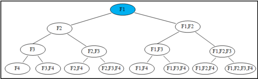
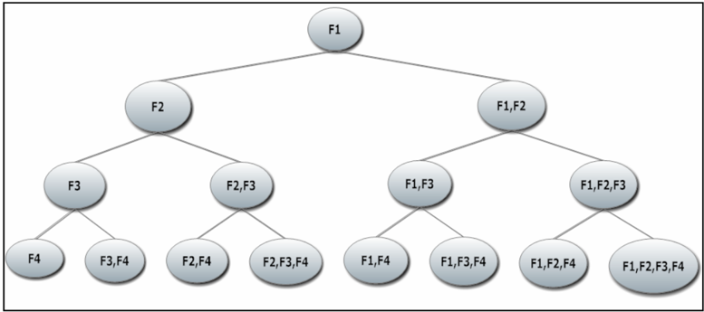
PRG algorithm is developed within context of this paper in order to find a solution to the problem of finding rule reduct in information systems. It is modified to find minimal set of rule reduction cases faster than the other algorithms. This algorithm uses tree structured data type. Before comparing objects properties with others, it uses a tree of features to map the search. The tree is developed according to the features and it shows all possible subsets of the features. When a rule reduct is detected, it prunes the next related branch of tree in specific system. Thus, not only finding redundant rule reducts is avoided, but also by decrease in work load fewer comparisons are needed to make. It is an effective way of finding minimal set of rule reducts. Tree diagram of an algorithm used in four-property information system is as below (Figure 3.1):

By looking Figure 3.1 it is seen that all subsets that belong to properties are located into tree. While examining rule reducts that belong to an object, in tree first of all, the way which will be followed starts from the root, and then goes to left child and finally the right child. Working principle of PRG algorithm can be told in detail as follows:

Step 0: Number of objects is assigned to be 1 i  .

Step 1: By building up the tree, all keys in nodes are assigned to be k=0.

Step 2: Node = Root.

Step 3: SEQUENCEOFACTION (Node)

Step 4: Set 1 i i   . If all objects are done, go to step 5, if not go to step 1.

Step 5: Finish.

SEQUENCEOFACTION (Node)

IF (RULEREDUCTION (Node))

Node is assigned to be Node.key = 1

The Rule Reduct in node is declared.

For all nodes connected to right child of the node and all nodes that are in same line with the mentioned node and includes all properties that the node has, assign Node.key = 1. This process makes redundant branches of tree pruned.

If Node.left  null

SEQUENCEOFACTION(Node.left)

If Node.right  null and Node.key = 0

SEQUENCEOFACTION(Node.right)

RULEREDUCTION (Node)

If Node.key = 1 return 'FALSE'

If for all j, i j  ; [( 1 1 , , i k j k a a  ) or ( 21 2 , , i k j k a a  ) or … t t i k j k a a , ,  )] then the case i ik kt ik k ik k d d a F a F a F t     , ,... , 2 1 2 1 is rule reduct. Return 'TRUE'

If for all j, i j  ; [( 1 1 , , i k j k a a  ) and ( 21 2 , , i k j k a a  ) and… t t i k j k a a , ,  )] and i j d d  then the case i ik kt ik k ik k d d a F a F a F t     , ,... , 2 1 2 1 is rule reduct. Return 'TRUE'

Else return 'FALSE'

4. COMPARISON PRG WITH RG AND MRG.

The Rule Reduct Generation (RG) and Modified Rule Generation (MRG) algorithms, that find rule reducts for an information system, are explained above. The Pruning Rule Generation (PRG) algorithm is developed as a more efficient and faster method to find minimal set of rule reducts. To compare the three methods, they are applied on Table 4.1 that is a decision table having four features, one decision value and five objects. This table and application of RG and MRG algorithms are taken from Guo and Chankong ( 2002)

Table 4.1: A Sample Decision Table

Object	F1	F2	F3	F4	Decision
1 x	0	0	1	3	0
2 x	0	1	1	1	1
3 x	1	2	2	0	1
4 x	0	1	0	2	2
5 x	0	0	0	1	2

At first RG algorithm is executed to find rule reducts. As known RG algorithm finds all possible rule reducts and this causes a lot of redundant rule reducts. The result of RG algorithm is shown in Table 4.2. There are 50 possible one-feature, two-feature and threefeature rule reducts.

Table 4.2: All possible rule reducts (RG)

	F1	F2	F3	F4	p	obj
One-featurer-reduct	NaN	NaN	NaN	3	0	1
	1	NaN	NaN	NaN	1	3
	NaN	2	NaN	NaN	1	3
	NaN	NaN	2	NaN	1	3
	NaN	NaN	NaN	0	1	3
	NaN	NaN	0	NaN	2	4
	NaN	NaN	NaN	2	2	4
	NaN	NaN	0	NaN	2	5
Two-featurer-reduct	0	NaN	NaN	3	0	1
	NaN	0	1	NaN	0	1
	NaN	0	NaN	3	0	1
	NaN	NaN	1	3	0	1
	NaN	1	1	NaN	1	2
	NaN	1	NaN	1	1	2
	NaN	NaN	1	1	1	2
	1	2	NaN	NaN	1	3
	1	NaN	2	NaN	1	3
	1	NaN	NaN	0	1	3
	NaN	2	2	NaN	1	3
	NaN	2	NaN	0	1	3
	NaN	NaN	2	0	1	3
	0	NaN	0	NaN	2	4
	0	NaN	NaN	2	2	4
	NaN	1	0	NaN	2	4
	NaN	1	NaN	2	2	4
	NaN	NaN	0	2	2	4
	0	NaN	0	NaN	2	5
	NaN	0	0	NaN	2	5
	NaN	0	NaN	1	2	5
Threefeaturer-reduct	NaN 0	NaN 0	0 1	1 NaN	2 0	5 1
	0	0	NaN	3	0	1
	0	NaN	1	3	0	1
	NaN	0	1	3	0	1
	0	1	1	NaN	1	2
	0	1	NaN	1	1	2
	0	NaN	1	1	1	2
	NaN	1	1	1	1	2
	1	2	2	NaN	1	3
	1	2	NaN	0	1	3
	1	NaN	2	0	1	3
	NaN	2	2	0	1	3
	0	1	0	NaN	2	4
	0	1	NaN	2	2	4
	0	NaN	0	2	2	4
	NaN	1	0	2	2	4
	0	0	0		2
	0			NaN		5
	0	0 NaN	NaN 0	1 1	2 2	5 5
	NaN	0	0	1	2	5

Unlike to RG, MRG algorithm can eliminate the redundant rule reducts. It is remembered that MRG begins to find one-feature rule reducts. In Table 4.3 all one-feature rule reducts are shown. Then MRG makes a revision on decision table and replace one-feature rule reducts with '*'. The Table 4.4 is handled as a revised decision table of Table 4.3.

F1	F2	F3	F4	P	obj
NaN	NaN	NaN	3	0	1
1	NaN	NaN	NaN	1
NaN	2	NaN	NaN	1
NaN	NaN	2	NaN	1	E
NaN	NaN	NaN	0	1	3
NaN	NaN	0	NaN	2	4
NaN	NaN	NaN			224

Table 4.3: One-feature rule reducts (MRG) Table 4.4: Revised decision table

Obj.no F1		F2	F3	F4d
一	0	0	1	串	0
2	0	1	1	1	1
3	*		*	*	1
4	0	1	*	*	2
5	0	0	*	1	2

After finding one-feature rule reducts, the decision table is revised then the revised table is used in MRG algorithm. Searching for two-feature rule reducts is executed and the twofeature rule reducts are shown in Table 4.5. As mentioned before, the decision table is revised again then Table 4.6 is reached.

Table 4.5: Two-feature rule reducts (MRG)

F1	F2	F3	F4	P	obj
NaN	0	1	NaN	0	1
NaN	1	1	NaN	1	2
NaN	1	NaN	1	1	2
NaN	NaN		1	1	2
NaN	0	NaN	1	2	5

Table 4.6: Revised decision table

Obj.no	F1	F2	F3	F4	d
1	0	0(*2)	1(*2)		0
2	0		1（*2,*2'）1（*2,*2"'）1	1(*2',*2")1
3	*	*	*	*	1
4	0	1	串	*	2
5l	0	0(*2)	*	1(*2)	2

The result of MRG algorithm is shown in Table 4.7. There are 12 possible one-feature and two-feature rule reducts. There is no three-feature rule reduct because all possible three- feature rule reducts are redundant. MRG algorithm eliminates all redundant rule reducts then it attains the minimal set of rule reducts as shown in Table 4.7.

Table 4.7: Minimal set of r-reducts (MRG)

	F1	F2	F3	F4	p	obj
Onefeaturer-reduct	NaN	NaN	NaN	3	0	1
	1	NaN	NaN	NaN	1	3
	NaN	2	NaN	NaN	1	3
	NaN	NaN	2	NaN	1	3
	NaN	NaN	NaN	0	1	3
	NaN	NaN	0	NaN	2	4
	NaN	NaN	NaN	2	2	4
Twofeaturer-reduct	NaN	0	1	NaN	0	1
	NaN	1	1	NaN	1	2
	NaN	1	NaN	1	1	2
	NaN	NaN	1	1	1	2
	NaN	0	NaN	1	2	5

Pruning Rule Reduction (PRG) algorithm also eliminates redundant rule reducts. It finds minimal rule reducts for an information system. The difference between MRG and PRG is the elimination method. MRG needs to revise the decision table but PRG uses a tree structured data type. This tree acts as a map for searching rule reducts. While processing the method, some branches of the tree is pruned, hence it means there is a redundant rule reduct. The branches that are declared as redundant, are not searched for rule reduction. Therefore, processing time is shortened. Finally, minimal set of rule reduction is reached by PRG in a less time than MRG.

The fourth object is marked in Table 4.8. The PRG algorithm is tried to find the rule reducts for that object. The searching methodology is indicated step by step.

Table 4.8: Searching the fourth object for rule reduction

Object	F1	F2	F3	F4	Decision
1 x	0	0	1	3	0
2 x	0	1	1	1	1
3 x	1	2	2	0	1
4 x	0	1	0	2	2
5 x	0	0	0	1	2

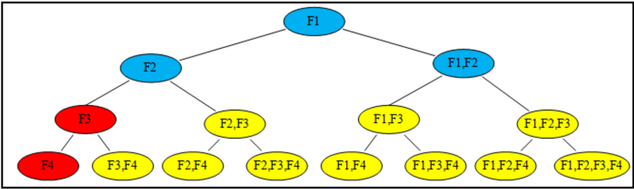
As it can be remembered PRG uses a tree structured data type. This tree that includes all subsets of the features is like a map for searching. In Figure 4.1 PRG tries to find a onefeature rule reduct for 4 x . The F1 value is 0 for 4 x and PRG decides there is no rule reduct for F1 feature.

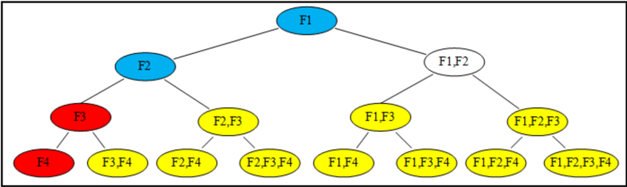
Searching the rule reducts traces an in-order path on the tree. The second step is done in Figure 4.2. The algorithm decides that F2 is not a rule reduct for 4 x .

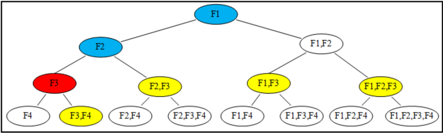
The third step is done for F3 . The value of F3 is 0 and PRG algorithm determines that F3 is a one-feature rule reduct for 4 x . After finding the rule reduction, the tree branches are pruned. Pruning process is useful to avoid from redundant rule reducts. When a rule reduct is detected, the tree node that shows the feature group is marked. The right child of the node and all brother nodes that include the feature group are pruned. This pruning process provides less searching processes, shorter time to terminate and minimal rule reducts. In Figure 4.3 the tree node F3 is declared as a one-feature rule reduct. After finding the rule reduction the tree nodes F3F4 , F2F3 , F1F3 , F1F2F3 are pruned, because they include F3 feature and cause redundant rule reducts.

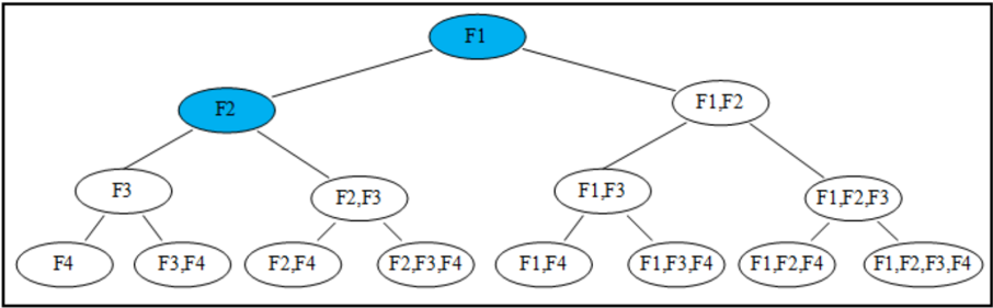
The next step is done for F4 feature. PRG algorithm determines that F4 is a one-feature rule reduct for 4 x . Then pruning process is begun and the tree nodes F2F4 , F2F3F4 , F1F4 , F1F3F4 , F1F2F4 , and F1F2F3F4 are pruned. Because these features include F4 feature and they are redundant rule reducts.

It is told above that the PRG traces the tree in-order direction. After finding rule reduct for F4 feature, it is expected that the algorithm will begin to search for F3F4 node. But since F3 is a one-feature rule reduct, the algorithm passes the right child. Then the right child of the F2 , F2F3 will be searched, but it is also pruned so this node and its right child F2F3F4 are passed. The next node is F2F4 , but by reason of one-feature rule reduct for F4 , it has been also pruned and it is passed. Finally in execution queue the node F1F2 is searched whether it is a rule reduct or not. It is not rule reduct, hence the algorithm does not make any process for this feature couple. The result of execution is shown in Figure 4.5. The other six nodes are not searched by PRG because they have been all pruned.

5. CONCLUSION

Rough Set Theory presents quite successful solutions for analysis and classifications of big data sets that consist of a large number of qualifications. By rule reduction technique; analyzing data becomes easier. However, detecting rule reduction cases in information system of big data sets is pretty complicated. In this paper, information about methods of rule reduction called RG and MRG is given. Beside their availability, the cases, in which these two methods are deficient, are explained. Methods for problems are as effective as their availability. And, approaches with huge costs are rarely preferred. PRG algorithm, which is developed in this paper for more efficient and useable approaches, fills the deficient part of the other two algorithms. By avoiding redundant rule reductions, PRG algorithm not only facilitates the analysis of information system, but also makes the problem solved in shorter time.

6. REFERENCES

Griffin, g and Chen,Z (1998) 'Rough set extension of Tcl for data mining', Knowledge-Based systems 11, 249-253

Grzymala-Busse,J. (1991) Managing Uncertainty in ExpertSystems Kluwer,Boston.

Grzymala-Busse, J(1992) 'LERS-a system for learning from examples based on Rough Sets', Intelligent Decision Support, Handbook of Applications and Advances of the Rough Sets Theory (Kluwer, Dordrecht) ,Vol. 3

Grzymala-Busse,J. and Wang,C.P. (1996) 'Classification and rule induction based on rough sets', IEEE Transaction on Knowledge and Data Engineering, 744-747

• Guo J.-Y. and Chankong V.(2002) 'Rough set-based approach to rule generation and rule induction', International Journal of General Systems, 31(6), 601-617
• Khoo, L.P, Tor, S.B. and Zhai, L.Y. (1999) 'Rough set-based approach to classification and rule induction', İnternational Journal of Advanced Manufacturing Technology 15 ,438-444
• Komorowski,J., Polkowski,L., Skowron,A. (1998) 'Rough Sets: A tutorial', In: RoughFuzzy Hybridization: A new method for decision making.,Springer-Verlag
• Kusiak,A (2000) Computational Intelligence in Design and Manufacturing (Wiley, New York), pp 498-527
• Kusiak, A and Tseng, T.L. (1999) 'Modeling approach to data mining', Proceeding of the Industrial Engineering and Production Management Conference,( Glasgow, Scotland), pp 113
• Lingras. P.J. (1996) ' Belief and probability based database mining', Proceeding of the Ninth Florida Artificial Intelligence Symposium, 316-320

Mrozek,A and Ekabek(1998) 'Rough sets in economic applications.' In: Polkowski and Skowron (Eds) 'Rough Sets in Knowledge Discovery 2: Applications, Case Studies and Software Systems,238-271(Verlag, Germany)

Mrozek,A and Plonka,L(1993)'Rough sets in image analysis', Foundations of Computing Decision Sciences, 18, (3-4 ), 259-273

Pawlak,Z (1982) 'Rough Sets', International Journal of Computer and Information Sciences 11 ,341-356

Pawlak,Z (1984)' On conflicts', International Journal of Man-Machine Studies, 21, 127-134

Pawlak, Z and Munakata ,T (1996) ' Rough Control, application of rough set theory to control': In::Zimmerman 'Proceedings of the Fourth European Congress on Intelligent Techniques and Soft Computing (EUFIT'96),209-218(verlag,Germany)

Polkowski,L.(2006) 'Rough Sets: mathematical foundations',Physica-Verlag

Slowinski,R and Stefanowski, J. (1989) 'Rough classification and incomplete information system', Mathematiical and Computer Modeling, 12, 1347-1357.

Slowinski, K.,Stefanowski, J, Swinski D (2002) 'Application of rule induction and rough sets to verification of magnetic resonance diagnosis', Fundamenta Informaticae , 53( 3-4),345-363

Wakulicz-Deja, A and Paszek,P. (1997) 'Diagnose progressive encephalopathy applying the rough set theory', International Journal of Medical Informatics 46 ,119-127

Yao, Y., Wong, .K.M. and Lin, T.Y.A. (1997) 'Review of Rough sets models', In: Lin, T.Y. and Cercone,N.,eds, Rough Sets and Data Mining-Analysis for Imprecise Data (Kluwe,Boston).

Ziarko,W (1993) 'Analysis of uncertain information in the framework of variable precision rough sets', Fund. Computing Decision Science 18 ,381-396