Qualitative Reasoning about Relative Direction on Adjustable Levels of Granularity

Till Mossakowski 1 and Reinhard Moratz 2

1

University of Bremen, Collaborative Research Center on Spatial Cognition (SFB/TR 8), Department of Mathematics and Computer Science, and DFKI GmbH, Enrique-Schmidt-Str. 5, 28359 Bremen, Germany.

[email protected]

2

University of Maine,

Department of Spatial Information Science and Engineering, 348 Boardman Hall, Orono, 04469 Maine, USA.

[email protected]

Abstract

Animportant issue in Qualitative Spatial Reasoning is the representation of relative direction. In this paper we present simple geometric rules that enable reasoning about relative direction between oriented points. This framework, the Oriented Point Algebra OPRA m , has a scalable granularity m . We develop a simple algorithm for computing the OPRA m composition tables and prove its correctness. Using a composition table, algebraic closure for a set of OPRA statements is sufficient to solve spatial navigation tasks. And it turns out that scalable granularity is useful in these navigation tasks.

Keywords:

Qualitative Spatial Reasoning, Constraint-based Reasoning, Qualitative Simulation

1 Introduction

The concept of qualitative space can be characterized by the following quotation from Galton [9]:

The divisions of qualitative space correspond to salient discontinuities in our apprehension of quantitative space.

If qualitative spatial divisions serve as knowledge representation in a reasoning system deductive inferences can be realized as constraint-based reasoning [24]. An important issue in such Qualitative Spatial Reasoning systems is the representation of relative direction[7], [1]. Qualitative spatial constraint calculi typically store their spatial knowledge in a composition table [24]. For a recent overview about Qualitative Spatial Reasoning (QSR) we refer to Renz and Nebel [24].

A new qualitative spatial reasoning calculus about relative direction, the Oriented Point Algebra OPRA m , which has a scalable granularity with parameter m ∈ N was presented in [15]. The motivation for this scalable granularity was that representing relatively fine distinctions was expected to be useful in more complex navigation tasks. It turned out to be difficult to analyze the reasoning rules for this calculus: The algorithm presented in the original paper [15] contained many gaps and errors. The algorithm presented in [8] is quite lengthy and cumbersome.

The paper is organized as follows: we will first give a short overview about OPRA m calculus. We start this with a definition for a coarse type ( m = 2 ), followed by the model for arbitrary m ∈ N . Then we will present a new compact algorithm which to performs OPRA m reasoning based on simple geometric rules, and prove its correctness. At the end we give an overview about several application that use the OPRA m calculus for spatial navigation simulations and discuss the adequateness of specific choices for the granularity parameter m .

2 The oriented point algebra

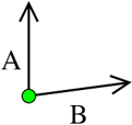
Objects and locations can be represented as simple, featureless points. In contrast, the OPRA m calculus uses more complex basic entities: It is based on objects which are represented as oriented points. It is related to a calculus which is based on straight line segments (dipoles) [21]. Conceptually, the oriented points can be viewed as a transition from oriented line segments with concrete length to line segments with infinitely small length [20]. In this conceptualization the length of the objects no longer has any importance. Thus, only the orientation of the objects is modeled. O-points , our term for oriented points, are specified as pair of a point and a orientation on the 2D-plane.

2.1 Qualitative O-Point Relations and Reasoning

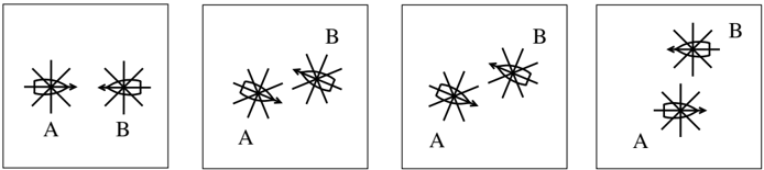
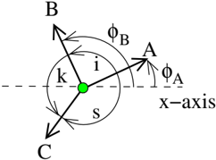
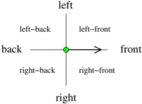
In a coarse representation a single o-point induces the sectors depicted in figure 1. 'front', 'back', 'left', and 'right' are linear sectors. 'left-front', 'right-front', 'leftback', and 'right-back' are quadrants. The position of the point itself is denoted as 'same'. This qualitative granularity corresponds to Freksa's double cross calculus [5, 25].

A qualitative spatial relative direction relation between two o-points is represented by two pieces of information:

• the sector (seen from the first o-point) in which the second o-point lies (this determines the lower part of the relation symbol), and
• the sector (seen from the second o-point) in which the first o-point lies (this determines the upper part of the relation symbol).

For the general case of the two points having different positions we use the following relation symbols:

front front , lf front , left front , lb front , back front , rb front , right front , rf front , front lf , lf lf , . . . , rf rf .

Altogether we obtain 8 × 8 base relations for the two points having different positions.

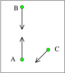
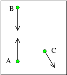
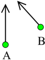
Then the configuration shown in figure 2 is expressed with the relation A lf rf B . If both points share the same position, the lower relation symbol part is the word 'same' and the upper part denotes the direction of the second o-point with respect to the first one as shown in figure 3.

Altogether we obtain 72 different atomic relations (eight times eight general relations plus eight with the o-points at the same position). These relations are jointly exhaustive and pairwise disjoint (JEPD). The relation front same is the identity relation.

In order to apply constraint-based reasoning to a set of qualitative spatial relations, the relations ideally should form a relation algebra [10] or a non-associative algebra [14, 11]. Such an algebra can be generated from a jointly exhaustive and pairwise disjoint set of base relations by forming the power set, giving the general relations, with bottom, top, intersection, union and complement of relations defined in the settheoretic way. Moreover, an identity base relation and a converse operation ( glyph[slurbelow] ) on base relations must be provided; the latter naturally extends to general relations. Finally,

if composition of base relations cannot be expressed using general relations (strong composition), this operation is approximated by a weak composition [22]:

glyph[negationslash]

where R b 1 ◦ R b 2 is the usual set theoretic composition

and R b is the set-theoretic relation corresponding to the abstract base relation b . For details we refer to [11].

The composition of relations must be computed based on the semantics of the relations. The compositions are usually computed only for the atomic relations; this information is stored in a composition table. The composition of compound relations can be obtained as the union of the compositions of the corresponding atomic relations. The compositions of the atomic relations can be deduced directly from the geometric semantics of the relations (see section 2.3).

O-point constraints are written as xRy where x, y are variables for o-points and R is a OPRA relation. Given a set Θ of o-point constraints, an important reasoning problem is deciding whether Θ is consistent , i.e., whether there is an assignment of all variables of Θ with dipoles such that all constraints are satisfied (a solution ). A partial method for determining inconsistency of a set of constraints Θ is the path-consistency method [13], which computes the algebraic closure on Θ . This method applies the following operation until a fixed point is reached:

where i, j, k are nodes and R ij is the relation between i and j . The resulting set of constraints is equivalent to the original set, i.e. it has the same set of solutions. If the empty relation occurs while performing this operation, Θ is inconsistent, otherwise the resulting set algebraically closed 1 [22]. Note that algebraic closure not always implies consistency, and indeed, [8] show that this implication does not hold for the OPRA calculus. Indeed, consistency in OPRA has been shown to be NP-hard even for scenarios in base relations [27], while algebraic closure is a polynomial approximation of consistency.

1 which means that it is path-consistent in the case that the algebra has a strong composition

2.2 Finer Grained O-Point Calculi

The design principle for the coarse OPRA calculus described above can be generalized to calculi OPRA m with arbitrary m ∈ N . Then an angular resolution of 2 π 2 m is used for the representation (a similar scheme for absolute direction instead of relative direction was designed by Renz and Mitra [23]). The granularity used for the introduction of the OPRA calculus in the previous section is m = 2 , the corresponding OPRA version is then called OPRA 2 .

To formally specify the o-point relations we use two-dimensional continuous space, in particular R 2 . Every o-point S on the plane is an ordered pair of a point p S represented by its Cartesian coordinates x and y , with x, y ∈ R and an orientation φ S .

glyph[negationslash]

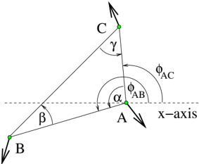
We distinguish the relative locations and directions of the two o-points A and B expressed by a calculus OPRA m according to the following scheme. For A , B with p A = p B , we define

where atan2 ( y, x ) is the angle between the positive x -axis and the point ( x, y ) , normalised to the interval ] -π, π ] . By the properties of atan2 , we get

modulo normalization to ] -π, π ] . In the sequel, we will normalize all angles to this interval, reflecting the cyclic order of the directions. Hence, e.g. -π stands for π . Moreover, in case that α > β , the open interval ] α, β [ will stand for ] α, π ] ∪ ] -π, β [ . For example, ] π 2 , -π 2 [ stands for ] π 2 , π ] ∪ ] -π, -π 2 [ .

Similarly, we enumerate directions by using the 4 m elements of the cyclic group Z 4 m . Each element of the cyclic group is interpreted as a range of angles as follows:

Conversely, for each angle α , there is a unique element i ∈ Z 4 m with α ∈ [ i ] m . If p A = p B , the relation A m ∠ j i B ( i, j ∈ Z 4 m ) reads like this: Given a granularity m , the relative position of B with respect to A is described by i and the relative position of A with respect to B is described by j . Formally, it represents the set of configurations satisfying glyph[negationslash]

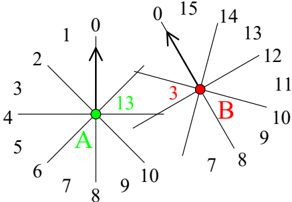
Figure 4 shows the resulting granularity for m = 4 . Using this notation, a simple manipulation of the parameters yields the converse operation ( m ∠ i j ) glyph[slurbelow] = m ∠ j i .

If p A = p B , the relation A m ∠ i B represents the set of configurations satisfying

8

Figure 4: Two o-points in relation A 4 ∠ 3 13 B

Hence the relation for two identical o-points A = B for arbitrary m ∈ N is A m ∠ 0 B . Using this notation a simple manipulation of the parameters yields the converse operation ( m ∠ i ) glyph[slurbelow] = m ∠ (4 m -i ) . The composition tables for the atomic relations of the OPRA m calculi can be computed using a small set of simple formulas detailed in the following subsection.

It should be mentioned that the passage from OPRA 1 to OPRA m ( m ≥ 2 ) is a qualitative jump: while OPRA 1 relations are preserved by all orientation-preserving affine bijections, for m ≥ 2 , OPRA m relations are only preserved by all anglepreserving affine bijections, see [20].

Proposition 1 Composition in OPRA is weak.

Proof. The configuration A 1 ∠ 0 0 B , B 1 ∠ 2 1 C and A 1 ∠ 3 3 C is realizable. However, given A and C as in Fig. 5, we have A 1 ∠ 3 3 C , but we cannot find B with A 1 ∠ 0 0 B and B 1 ∠ 2 1 C : by A 1 ∠ 0 0 B , B 's carrier line is the same as A 's, and the two o-points face each other. But then, B 1 ∠ 2 1 C is not possible, since B would have to be located in the back of C .

The argument easily generalizes to OPRA m by considering A m ∠ 0 0 B , B m ∠ 2 m 1 C and A m ∠ 4 m -1 4 m -1 C . ✷

2.3 Simple geometric rules for reasoning in OPRA m

The composition table can be viewed as a list (set) of all relation triples Ar ab B , Br bc C , Cr ca A for which r ab , r bc , and r ca are consistent ( A , B , and C being arbitrary o-points on the R 2 plane). In the literature, there are two algorithms for computing the composition table: [19] presents a fairly simple algorithm, which, however, is error-prone, and [8] provide a correct algorithm, which however is based on a complicated case distinction with dozens of cases (the paper is 29 pages long, 22 of which are devoted to the algorithm and its correctness!).

We give an algorithm that is both correct and simpler than the two existing algorithms.

The first ingredient of the algorithm is a detection of complete turns. We define

This definition determines complete turns in the following sense:

1. turn m ( i, j, k ) implies that for any choice of one of the three angles in its interval, a suitable choice for the other two exists such that all three add up to 0 .

Recall that angles are normalized into ] -π, π ] .

Proof. We prove the first statement by a case distinction. Case 1: both i and j are even. This means that [ i ] m = { 2 π i 4 m } and [ j ] m = { 2 π j 4 m } . Hence,

∃ α ∈ [ i ] m , β ∈ [ j ] m , γ ∈ [ k ] m . α + β + γ = 0 iff ∃ γ ∈ [ k ] m . 2 π i + j 4 m + γ = 0 iff i + j + k = 0 iff turn m ( i, j, k )

Case 2: i is odd and j is even. This means that [ i ] m =]2 π i -1 4 m , 2 π i +1 4 m [ and [ j ] m = { 2 π j 4 m } . Hence,

∃ α ∈ [ i ] m , β ∈ [ j ] m , γ ∈ [ k ] m . α + β + γ = 0 iff ∃ γ ∈ [ k ] m . -2 π j 4 m -γ ∈ ]2 π i -1 4 m , 2 π i +1 4 m [ iff ∃ γ ∈ [ k ] m . γ ∈ ]2 π -i -j -1 4 m , 2 π -i -j +1 4 m [ iff ∃ γ ∈ [ k ] m . γ ∈ [ -i -j ] m iff k = -i -j iff turn m ( i, j, k )

Case 3: i is even and j is odd: analogous to case 2.

Case 4: both i and j are odd. This means that [ i ] m =]2 π i -1 4 m , 2 π i +1 4 m [ and [ j ] m = ]2 π j -1 4 m , 2 π j +1 4 m [ . Hence, m

∃ α ∈ [ i ] m , β ∈ [ j ] m , γ ∈ [ k ] m . α + β + γ = 0 iff ∃ γ ∈ [ k ] m . γ ∈ ]2 π -i -j -2 4 m , 2 π -i -j +2 4 m [ iff ∃ γ ∈ [ k ] m . γ ∈ [ -i -j -1] m ∪ [ -i -j ] m ∪ [ -i -j +1] iff k ∈ {-i -j -1 , -i -j, -i -j +1 } iff turn m ( i, j, k )

The second statement is straightforward when inspecting the proof above. ✷

Next, we turn to triangles. In a triangle, the sum of angles is always π . Moreover, all angles have the same sign. We include the degenerate case where two angles are 0 and the remaining one is π (this corresponds to three points on a line), but we exclude the case of three angles being π (this is not geometrically realizable). This leads to the following definitions:

glyph[negationslash]

Here, the angle π also has sign 0 , which corresponds to the geometric intuition and to the fact that the choice between -π and π to represent this angle is rather arbitrary.

From the above discussion, it is then straightforward to see

Proposition 3

triangle m ( i, j, k ) iff ∃ α ∈ [ i ] m , β ∈ [ j ] m , γ ∈ [ k ] m . there exists a triangle with angles α, β, γ

Algorithm 1 now gives the complete algorithm for computing OPRA m compositions. Note that we have slightly rephrased the definition of turn m ( i, j, k ) , the new version already taking care of our convention regarding the cyclic group Z 4 m and thus being directly implementable as a computer program using the usual integers instead of Z 4 m .

Theorem 4 Algorithm 1 computes composition in OPRA m .

Proof.

Case opra ( m ∠ i, m ∠ k, m ∠ s ) . Since the points of all o-points are the same, their direction must add up to a complete turn. More precisely, the configuration m ∠ i, m ∠ k, m ∠ s is realizable iff there are o-points A , B and C with p A = p B = p C , φ B -φ A ∈ [ i ] m , φ C -φ B ∈ [ k ] m , and φ C -φ A ∈ [ s ] m . Since for such A , B and C , ( φ B -φ A ) + ( φ C -φ B ) -( φ C -φ A ) = 0 (i.e. we have a complete turn), by Proposition 2 this is in turn equivalent to turn m ( i, k, -s ) .

Cases opra ( m ∠ i, m ∠ k, m ∠ t s ) , opra ( m ∠ i, m ∠ l k , m ∠ s ) and opra ( m ∠ j i , m ∠ k, m ∠ s ) . Since sameness of points is transitive, these cases are not realizable.

Algorithm 1 Checking entries of the OPRA m composition table

triangle ( i, j, k ) iff

glyph[negationslash]

∃ 0 ≤ u, v, w < 4 m.turn m ( u, -i, s ) ∧ turn m ( v, -k, j ) ∧ turn m ( w, -t, l ) ∧ triangle m ( u, v, w )

Cases opra ( m ∠ i, m ∠ l k , m ∠ t s ) , opra ( m ∠ j i , m ∠ k, m ∠ t s ) and opra ( m ∠ j i , m ∠ l k , m ∠ s ) . We here only treat the case opra ( m ∠ i, m ∠ l k , m ∠ t s ) ; the other cases being analoguous. The configuration A m ∠ iB, B m ∠ l k C, A m ∠ t s C is realizable iff

We now show that ( ∗ ) is equivalent to

Assume ( ∗ ) . By p A = p B , we have φ BC = φ AC and φ CB = φ CA ; from the latter, we also get l = t . Moreover, ( φ B -φ A ) + ( φ BC -φ B ) -( φ AC -φ A ) = 0 is a

turn, and by Proposition 2, we get turn m ( i, k, -s ) . Conversely, assume l = t and turn m ( i, k, -s ) . By Proposition 2, there are angles α, β, γ with α ∈ [ i ] m , β ∈ [ k ] m and γ ∈ [ -s ] m . Choose A arbitrarily. Then define B by p B = p A and φ B = α -φ A . Then choose p C on the half-line starting from p A and having angle β to B and -γ to A . Finally, choose φ C such that φ CA -φ C = φ CB -φ C ∈ [ t ] m = [ l ] m . This ensures the conditions of ( ∗ ) .

glyph[negationslash]

Figure 7: p A = p B = p C

Case opra ( m ∠ j i , m ∠ l k , m ∠ t s ) . We need to show that the existence of a configuration A m ∠ j i B , B m ∠ l k C and A m ∠ t s C is equivalent to

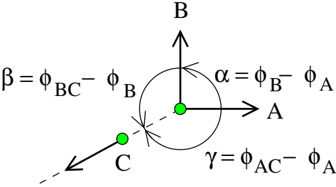
Given A m ∠ j i B , B m ∠ l k C and A m ∠ t s C , let α , β and γ be the angles of the triangle p A p B p C , that is,

Let u, v, w ∈ Z 4 m be such that α ∈ [ u ] m , β ∈ [ v ] m and γ ∈ [ w ] m . By Proposition 3, triangle m ( u, v, w ) . At the corners of the triangle p A p B p C , the following complete turns can be formed:

• ( φ AB -φ AC ) -( φ AB -φ A ) + ( φ AC -φ A ) , corresponding to turn m ( u, -i, s ) by Proposition 2,
• ( φ BC -φ BA ) -( φ BC -φ B )+( φ BA -φ B ) , corresponding to turn m ( v, -k, j ) ,
• ( φ CA -φ CB ) -( φ CA -φ C ) +( φ CB -φ C ) , corresponding to turn m ( w, -t, l ) .

This shows ( ∗∗ ) . Conversely, assume ( ∗∗ ) . By triangle m ( u, v, w ) and Proposition 3, we can choose p A , p B and p C such that

Since turn m ( u, -i, s ) , by Proposition 2, we can find α A , β A and γ A such that α A + β A + γ A = 0 and α A ∈ [ -i ] m , β A ∈ [ s ] m and γ A ∈ [ u ] m . From Proposition 2(2), we obtain that it is possible to choose γ A = φ AB -φ AC (note that the latter angle is also in [ u ] m ). Put φ A := φ AB + α A , then φ AB -φ A = -α A ∈ [ i ] m , and φ AC -φ A = ( φ AB -φ A ) -( φ AB -φ AC ) = -α A -γ A = β A ∈ [ s ] m . φ B and φ C can be chosen similarly, fulfilling the constraints given by j and k resp. l and t . ✷

Using Algorithm 1, a composition table for OPRA m can be computed by enumerating all possible triples and only keeping those for which the predicate opra holds. Moreover, given a pair of OPRA m relations, by enumerating all possible third OPRA m relations and testing with the predicate opra , also the composition of two relations can be computed.

The run time of the predicate opra is O ( m 3 ) , since the algorithm contains an existential quantification over the variables u , v , w ranging from 0 to 4 m -1 . However, the existential quantification can be replaced by a constant number of case distinctions: e.g. we look for u such that turn m ( u, -i, s ) . But since u -i + s must add up to -1 , 0 or 1 , it is clear that u must be taken from the set { i -s -1 , i -s, i -s +1 } . As a result, we get an improved run time that is constant. This holds only when assuming a register machine with arithmetic operations executed in constant time. For a Turing machine with binary representations of numbers, basic arithmetic operations take time log m . Then the run time is O (log m ) .

The computation of the composition of two relations needs to enumerate all possible third relations, and then check each triple in constant time. Since there are (4 m ) 2 +4 m relations, this takes O ( m 2 ) time, which is the same time as in [8]. Again, for Turing machines, this multiplies by a factor of log n , hence we get an overall running time of O ( m 2 log m ) . Of course, the same remark applies to the algorithm of [8].

AHaskell version of the opra algorithm (also implementing the above optimization of the existential quantification) can be downloaded at http://quail.rsise. anu.edu.au .

The OPRA calculus can be used to express many other qualitative position calculi [4].

3 Applications of the OPRA calculus

Spatial knowledge expressed in OPRA can be used for deductive reasoning based on constraint propagation (algebraic closure), resulting in the generation of useful indirect knowledge from partial observations in a spatial scenario. Several researchers developed applications using the OPRA calculus. We will give a short overview and then make some concluding comments about the first OPRA calculus applications in our conclusion section that follows.

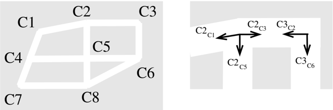
In a simple application by L¨ ucke et. al. [12] for benchmarking purposes between different spatial calculi, a spatial agent (a simulated robot, cognitive simulation of a biological system etc.) explores a spatial scenario. The agent collects local observations and wants to generate survey knowledge. Fig. 9 shows a spatial environment consisting of a street network. The notation C 2 C 1 refers to the o-point at position C 2 with an intrinsic orientation towards point C 1 . In this street network some streets continue straight after a crossing and some streets meet with orthogonal angles. These features are typical of real-world street networks and can be directly represented in OPRA 2 expressions about o-points that constitute relative directions of o-points located at crossings and pointing to neighboring (e.g. visible) crossings. For example two relations corresponding to local observations referring to the street network part depicted in Fig. 9 are: C 2 C 3 front front C 3 C 2 and C 2 C 3 right same C 2 C 5 . Spatial reasoning in this spatial agent simulation uses constraint propagation (e.g. algebraic closure computation) to derive indirect constraints between the relative location of streets which are further apart from local observations between neighboring streets. The resulting survey knowledge can be used for several tasks including navigation tasks. The details of this scenario can be found in L¨ ucke et. al. [12].

A related application developed by Wallgr¨ un [26] uses Qualitative Spatial Reasoning with OPRA to determine the correct graph structure from a sequence of local observations by a simulated robot collected while moving through an environment consisting of hallways. These hallway networks are analogous to the street networks of L¨ ucke et. al., but the local observation are modeled in a more complex but more

realistic way. The identity of a crossing revisited after a cyclic path is not given but has to be inferred which makes navigation much more challenging. Since there are many ambiguities left, the task is to track the multiple geometrically possible topologies of the network during an incremental observation. Thus, the goal of Wallgr¨ un's qualitative mapping algorithm is to process the history of observations and determine all route graph hypotheses which can be considered valid explanations so far. This consistency checking can be based on qualitative spatial reasoning about positions. The local relative observation are modeled based on OPRA 2 expressions about o-points in a similar way like in the street network described above.

A comprehensive simulation which uses the OPRA 4 calculus for an important subtask was built by Dylla et. al. [2]. Their system called SailAway simulates the behavior of different vessels following declarative (written) navigation rules for collision avoidance. This system can be used to verify whether a given set of rules leads to stable avoidance between potentially colliding vessels The different vessel categories that determine their right of way priorities are represented in an ontology. The movement of the vessels is described by a method called conceptual neighborhood-based reasoning (CNH reasoning). CNH reasoning describes whether two spatial configurations of objects can be transformed into each other by small changes [6], [9]. A CNH transformation can be a object movement in a short period of time. Fig. 10 shows a CNH transition diagram which represents relative trajectories of two rule following vessels. The depicted sequence between two vessels A and B is:

A 4 ∠ 0 0 B → A 4 ∠ 1 1 B → A 4 ∠ 2 2 B → A 4 ∠ 3 3 B . Based on this qualitative representation of trajectories, CNH reasoning is used as a simple, abstract model of the navigation of the potentially colliding vessels in the SailAway simulator [2]) 2 .

These three applications above make use of qualitative spatial reasoning with OPRA 2 or OPRA 4 in simulated spatial agent scenarios. The granularity m = 2 can model straight continuation and right angles which are important for representing idealized street networks. The granularities m = 2 and m = 4 also correspond to earlier work about computational models of linguistic projective expressions (left, right, in front, behind) by Moratz et. al. [16] [18]. The applications presented in this section could benefit from additional qualitative relative distance knowledge. The TPCC calculus presented by Moratz & Ragni [17] is a first step towards this direction. However,

2 An earlier version of qualitative navigation simulation by Dylla and Moratz can be found in [3]

in contrast to our new results for the OPRA m calculus the TPCC calculus only has a complex, manually derived and therefore unreliable composition table.

4 Summary and Conclusion

We presented a calculus for representing and reasoning about qualitative relative direction information. Oriented points serve as the basic entities since they are the simplest spatial entities that have an intrinsic orientation. Sets of base relations can have adjustable granularity levels in this calculus. We provided simple geometric rules for computing the calculi's composition based on triples of oriented points.

We gave a short overview about three first applications that are based on oriented points and their relative position represented as OPRA m relations with granularity m = 2 , or m = 4 which seem to be suited for linguistically inspired spatial expressions.

Acknowledgment

The authors would like to thank Lutz Frommberger, Frank Dylla, Jochen Renz, Diedrich Wolter, Dominik L¨ ucke, and Christian Freksa for interesting and helpful discussions related to the topic of the paper. The work was supported by the DFG Transregional Collaborative Research Center SFB/TR 8 'Spatial Cognition' and by the National Science Foundation under Grant No. CDI-1028895.

References

1. E. Clementini, P. Di Felice, and D. Hernandez. Qualitative Represenation of Positional Information. Artificial Intelligence , 95:317-356, 1997.
2. F. Dylla, L. Frommberger, J. O. Wallgr¨ un, D. Wolter, S. W¨ olfl, and B. Nebel. SailAway: Formalizing Navigation Rules. In Proc. of the AISB'07 Artificial and Ambient Intelligence Symposium on Spatial Reasoning and Communication , 2007.
3. F. Dylla and R. Moratz. Exploiting Qualitative Spatial Neighborhoods in the Situation Calculus. In C. Freksa, M. Knauff, B. Krieg-Br¨ uckner, B. Nebel, and T. Barkowsky, editors, Proc. of Spatial Cognition 2004 , pages 304-322, 2005.
4. Frank Dylla and Jan-Oliver Wallgr¨ un. On generalizing orientation information in OPRA m . In KI-2006: Proceedings of the 29th Annual German Conference on Artificial Intelligence , Lecture Notes in Artificial Intelligence. Springer, 2006.
5. C. Freksa. Using orientation information for qualitative spatial reasoning. In A. U. Frank, I. Campari, and U. Formentini, editors, Theories and methods of spatio-temporal reasoning in geographic space , volume 639 of Lecture Notes in Comput. Sci. , pages 162-178. Springer, 1992.

1. Christian Freksa. Conceptual neighborhood and its role in temporal and spatial reasoning. In Madan G. Singh and Luise Trav´ e-Massuy` es, editors, Proceedings of the IMACS Workshop on Decision Support Systems and Qualitative Reasoning , pages 181-187, North-Holland, Amsterdam, 1991. Elsevier.
2. Christian Freksa. Using orientation information for qualitative spatial reasoning. In A. U. Frank, I. Campari, and U. Formentini, editors, Theories and methods of spatio-temporal reasoning in geographic space , pages 162-178. Springer, Berlin, 1992.
3. Lutz Frommberger, Jae Hee Lee, Jan Oliver Wallgrn, and Frank Dylla. Composition in OPRA m . Technical report, SFB/TR 8, University of Bremen, 2007.
4. Antony Galton. Qualitative Spatial Change . Oxford University Press, 2000.
5. P. Ladkin and R. Maddux. On binary constraint problems. Journal of the Association for Computing Machinery , 41(3):435-469, 1994.
6. G. Ligozat and J. Renz. What Is a Qualitative Calculus? A General Framework. In C. Zhang, H. W. Guesgen, and W.-K. Yeap, editors, Proc. of PRICAI-04 , pages 53-64, 2004.
7. D. L¨ ucke, R. Moratz, and T. Mossakowski. A simulator for qualitative reasoning in street network. Technical report, SFB/TR 8, University of Bremen, 2010.
8. A. K Mackworth. Consistency in networks of relations. Artificial Intelligence , 8:99-118, 1977.
9. R. Maddux. Relation Algebras . Stud. Logic Found. Math. Elsevier Science, 2006.
10. R. Moratz. Representing Relative Direction as a Binary Relation of Oriented Points. In G. Brewka, S. Coradeschi, A. Perini, and P. Traverso, editors, Proc. of ECAI-06 , volume 141 of Frontiers in Artificial Intelligence and Applications , pages 407-411. IOS Press, 2006.
11. R. Moratz, K. Fischer, and T. Tenbrink. Cognitive Modeling of Spatial Reference for Human-Robot Interaction. International Journal on Artificial Intelligence Tools , 10(4):589-611, 2001.
12. R. Moratz and M. Ragni. Qualitative Spatial Reasoning about Relative Point Position. J. Vis. Lang. Comput. , 19(1):75-98, 2008.
13. R. Moratz and T. Tenbrink. Spatial reference in linguistic human-robot interaction: Iterative, empirically supported development of a model of projective relations. Spatial Cognition and Computation , 6(1):63-107, 2006.
14. Reinhard Moratz. Representing relative direction as a binary relation of oriented points. In Gerhard Brewka, Silvia Coradeschi, Anna Perini, and Paolo Traverso, editors, ECAI , volume 141 of Frontiers in Artificial Intelligence and Applications , pages 407-411. IOS Press, 2006.

1. Reinhard Moratz, Dominik L¨ ucke, and Till Mossakowski. Oriented straight line segment algebra: Qualitative spatial reasoning about oriented objects. CoRR , abs/0912.5533, 2010. Submitted 13 Mar 2010 to Artificial Intelligence Journal, 75 pages.
2. Reinhard Moratz, Jochen Renz, and Diedrich Wolter. Qualitative spatial reasoning about line segments. In Proceedings of ECAI 2000 , pages 234-238, 2000.
3. J. Renz and G. Ligozat. Weak composition for qualitative spatial and temporal reasoning. In CP 2005 , 2005.
4. J. Renz and D. Mitra. Qualitative direction calculi with arbitrary granularity. In Proceedings PRICAI 2004 (LNAI 3157) , September 2004.
5. J. Renz and B. Nebel. Qualitative Spatial Reasoning Using Constraint Calculi. In M. Aiello, I. Pratt-Hartmann, and J. van Benthem, editors, Handbook of Spatial Logics , pages 161-215. Springer, 2007.
6. A. Scivos and B. Nebel. The finest of its class: The natural point-based ternary calculus for qualitative spatial reasoning. In C. Freksa, M. Knauff, B. Krieg Br¨ uckner, B. Nebel, and T.Barkowski, editors, Spatial Cognition , volume 3343 of Lecture Notes in Comput. Sci. , pages 283-303. Springer, 2004.
7. Jan Oliver Wallgr¨ un. Qualitative spatial reasoning for topological map learning. Spatial Cognition and Computation .
8. D. Wolter and J. H. Lee. On Qualitative Reasoning about Relative Point Position. accepted for publication in Artif. Intell.