Quasi-Bayesian Strategies for Efficient Plan Generation: Application to the Planning to Observe Problem

Fabio Cozman Eric Krotkov Robotics Institute, School of Computer Science - Carnegie Mellon University Pittsburgh, PA 15213

Abstract

Quasi-Bayesian theory uses convex sets of probability distributions and expected loss to represent preferences about plans. The the­ ory focuses on decision robustness, i.e., the extent to which plans are affected by devi­ ations in subjective assessments of probabil­ ity. G en e r a ti n g a plan means enumerating the actions to be taken and providing infor­ mation about the robustness of the actions. The present work presents plan generation problems that can be solved faster in the Quasi-Bayesian framework than within usual Bayesian theory. We investigate this on the planning to observe problem, i.e., an agent must decide whether to take new observa­ tions or not. The fundamental question is: How, and how much, to search for a "best" plan, based on the precision of probability assessments? Plan generation algorithms are derived in the context of material classifica­ tion with an acoustic robotic probe. A pack­ age that constructs Quasi-Bayesian plans is available through anonymous ftp.

1 INTRODUCTION

Agents choose a plan of action by comparing its pos­ sible outcomes against the outcomes of other plans. Bayesian theory suggests that the basis for such com­ parisons is expected loss with a single probability dis­ tribution. Quasi-Bayesian theory, as axiomatized by Giron and Rios [Giron an d Rios, 1980], also relies on expected loss, but uses a convex set of pro ba b i lity dis­ tributions to represent the agent's beliefs. Many s chol ­ ars agree that assuming an agent uses a single proba­ bility distribution is too restrictive [Breese and Fertig, 1991; Levi, 1980; Shafer, 1987]. But there has been little agreement on how to make decisions with several distributions; many seem to think that theories with several d istr i b u t io n s will always lead to intractable de­ cision making problems.

Recently, great attention has been given to Robust Bayesian Statistics, which uses Quasi-Bayesian sets of distributions to represent imprecision of subjectivr probability assessments [Berger, 1985; Walley, 1991]. A robust decision is one that can be safely tahm dc�­ spite the imprecision in the probability a s ses sme nt s : a non-robust decision is one that may produce wildly dif­ ferent results depending on the adopted distribution.

In this paper, we explore a Quasi-Bayesian approach to plan generation. Generating a plan means enumerat­ ing the actions to be taken and providing information about the robustness of the actions. Our approac:h puts less emphasis on the search for unique "best" dc·'­ cisions than the usual Bayesian approach. Essentially, the agent is required to choose admissible decisions and to monitor and report robustness of these decisiot1s. We clarify the terms involved in this requirement in sections 2 and 3.

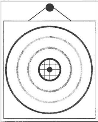
The central point of this work can be expressed hy a short fable. Suppose two archers try to h i t a target (Figure 1). The first archer, a Bayesian, considers that hitting the center of the target is the o n l y satisfactor.v result and orders a new, expensive bow. But the judgP only detects if an archer hits the hatched r e g i o n . If both archers hit the hatched region, the judge con�icl­ ers them tied and calls o t h e r procedures to solve' tlw dispute. That does not prevent the Ba y es i a n archer from trying to hit the center. The ser:oncl archer, a New Quasi-Bayesian archer, tries simply to n�ac:h tlw hatched circle with a cheap how. The 1'\<�w Qnasi­ Bayesian strategy seems wiser given the lack of pn·ti­ sion of the target.

Our main contribution is to show that the An:lwrs Fable can be formalized for the planning to observe problem. The analogy here is t ha t a point in the tar­ get corresponds t o a distribution: the Bayesian agc'ut has one, the Quasi-Bayesian agent has many. The·· Bayesian seeks an answer to the question, how to r:rc·­ ate an optimal sequence of actions'? Such a question is very demading computationally. The Quasi-Baycsimt is a t t en ti v e to the limitations of real probability as­ sessments and seeks an answer to the question, hem· t(l create a sequence of admissible actions and qnantii\

the robustness of such actions? The s ur pr is i ng result is that we can answer the latter question without ex­ amining the full solution for the former question. To illustrate the details of our solution, we apply it to the planning to observe p r o b l e m for material classification with a robotic probe.

2 THE QUASI-BAYESIAN FRAMEWORK

Consider this problem: an agent must choose a plan ai b e fo r e the state of the world is known; after the state is revealed to be 61, the agent pays a loss l;1. T h e losses indicate the preferences of the agent. How should the agent compare two plans, a1 and a2? Quasi-Bayesian theory asserts that there is a n o nempty convex set K of p r o ba b ility distributions which summarizes the ag e n t ' s beliefs. The set K is such that, for pl ans a1 a n d a2, a1 is at least as preferred as az iff E[llj] 2: E[lzj] for every p r o ba bi l i ty distribution K, where E[·] denotes expected loss. Giron and Rios pr e s en t a s e t of axioms that validate the preferences of a Q uas i -B a ye s i a n agent [Giron and Rios, 1980]. The set of probability distri­ butions K is called the credal s et [Levi, 1980]. The representation of preferences conditional on a state is characterized by a convex set of posterior distributions obtained through application of Bayes rule to each one of the distributions in the set of priors1.

There a r e other methods for creating sets of pro b a ­ bility distributions: inner and outer measures [Good, 1983; Halpern and Fagin, 1992; Ruspini, 1987; Su p ­ pes, 1974], i n te rv a l s of probability (commonly gener­ ated by lower probability) [Breese and Fertig, 1991; Chrisman, 1995; Fine, 1988; H. E. K y b urg Jr., 1987;

1 An introduction to technical aspects of Quasi-Bayesian theory, with a larger list of references, can be found at http:/ /www.cs.cmu.edu/-fgcozman/qBayes.html.

Halpern and Fagin, 1992; Smith, 1961], lower expec­ tations [ W alle y , 1991]. The belief functions used in Dempster-Shafer theory [Rus p i ni, 1987; Shafer, 1987] h a v e different interpretations but can be represented as sets of probabilities. Qu a s i -B ay e s i a n models gener­ a l i ze these i d e a s . Given a Quasi-Bayesian convex set of probability distributions, a probability interval can be created for every event A b y defining lower and upper b o u nds :

In a different d ir ect i o n , m o r e g en e r a l models than tlw Qu a s i -B a y e s i a n one can be created, for i n st an c e the­ ories of decision which use s im u l tan e ou s sets of losses and probabilities [Levi, 1980; Seidenfeld, 1993].

There are some basic reasons for adopting a Q u as i ­ B a ye s ian m o d e l [S e i de n feld and Wasserman, 1993]. First, Quasi-Bayesian theory builds a realistic account of the i m p e rf ect i on s in an a g e nt ' s beliefs. It can lw u s ed to r e p r e s e n t poor elicitation of preferences and situations of indifference among a c t io n s . Second, ro­ bustness studies can be f o r m a l i z ed through this model [Berger, 1985]. Third, the theory can re p rese nt tlw d i s p a r a te opinions of a group of agents [Levi, 1980].

3 BUILDING A NEW APPROACH TO DECISION-MAKING

A B a ye s i an agent can always say that a plan is better than, worse t h a n , or equal to another plan. A Quasi­ B a ye s i a n agent may b e in a d i ff e r ent situation. Con­ sider two p la n s , a1 and a2, and two di s tr ibu t io n s J>i and p2 in the c r eda l s e t . S u p p o s e p l an a1 has smaller expected loss than p l an a2 w i t h respect to a probabil­ ity d i s t r ib u t i o n p1, but a2 has smaller expected loss w i th respect to another p r o b a bilit y di st r i b u tion p2. In this ca s e , a1 and a2 ar e not comparable by expected loss; both are admissible. What should be done?

Reactions to this question vary. F e r t i g and Breese�, in their work with interval probabilities, simply w­ p o r t all admissible pl an s [ B r e es e and Fertig, 1991; Fertig and B r e ese , 1990]. This leaves the actual ac­ tions unspecified. Levi ar g u es t h a t p l a n s s hou l d not on l y be admissible, but also be op t i m a l with respect to some di s t r i b u t i on in the credal set. He calls such a plan E -ad m i ss i b l e [ Levi, 1980]. Since t h e r e may lw s e v e r a l E-admissible plans, Levi s u g g e s t s secowlary guidelines that enforce "security". Others have� sug-­ gested the agent should minimize the maximum possi­ ble value of expected loss, an approach common in Ro­ bust Bayesian Statistics under the name o ff -m in i max [Berger, 1985].

We s ugg e s t that Quasi-Bayesian strategies sh o u l d spcr:­ ify the admissible decisions and allow the agent to monitor the robustness of such decisions. Tlws<� an� t h e two requirements on a plan. There should be no ar­ tificially enforced preference among admissible plans:

any admissible plan provide useful guidance if an ac­ tion must be chosen. Robustness should always be monitored; what use is a "best" plan if it is based on a skewed set of assumptions? As long as a plan provides a method for the detection of non-robust situations, the agent can pick the first admissible decision that ad­ mits convenient manipulation in the time available for decision-making. We call this the New Quasi-Bayesian strategy.

The strategy above contains important elements of decision-making as it must be exercised by finite, bounded agents. The agent is required to produce an admissible answer as quickly as possible, and have that as a default solution, as usually required in any­ time planning. Further, the agent is required to detect the situations that require additional computation and refinement: those are the non-robust situations.

Compared to the Bayesian strategy, the New Quasi­ Bayesian strategy has some remarkable differences. The Bayesian strategy will always be appropriate if there is total confidence on the precision of probabil­ ity assessments. If that is not the case, the Bayesian strategy calls for a decision analysis of the value of further computation and/or introspection [Beckerman and Jimison, 1989; Horvitz, 1989; Matheson, 1968; Russell and Wefald, 1991]. Such meta-analysis re­ quires probabilities over probabilities, which may be harder to elicit than a simple set of bounds on distri­ butions.

So far we have specified the New Quasi-Bayesian strat­ egy, but it is still unclear how we can use this strategy in any decision problem. In order to do so, we must be able to quickly generate actions and monitor robust­ ness. Ideally, we must be able to do so faster than the usual Bayesian solution, which involves generating ac­ tions and either checking the sensitivity of such actions or checking the meta-analysis for those actions. In the remainder of the paper, we show that these goals are met for the planning to observe problem with Gaussian measurements. This is a classic Markov decision prob­ lem; although we describe the solution for univariate data, the ideas readily extend to multivariate data.

4 PLANNING TO OBSERVE WITH GAUSSIAN MEASUREMENTS

We now demonstrate our approach to decision-making on the planning to observe problem described as follows:

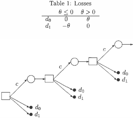
A series of independent r e a l -v al u e d observations Xi is available to an agent; each observation costs c units of loss and is normally distributed with known variance 1/r and unknown mean B. We indicate this by Xi ""' N(xi; B, 1/r). The agent wants to know whether B is larger or equal, or smaller than zero. At any point, the agent can take a new observation or stop and decide: Smaller ( d o ) and Larger (di). When a decision is made, the loss L(B, di) is defined by Table 1.

Figure 2 illustrates the dynamics of the problem. At any point, the agent is facing the same question as to whether a decision should be made or an observation should be taken. We want to find a sequence of actions for the agent.

4.1 THE CREDAL SET

Prior beliefs about B translate into a convex set of probability distributions, the credal set. A realistic model for prior beliefs would take a credal set large enough to represent the non-specificity of the agent's beliefs. Consider the convex set of distributions com­ posed of Gaussian distributions with mean between 1<1 and J-1 2 , and variance 1 j 1:

To create a convex set of distributions, it may be neces­ sary to use convex combinations of distributions". To build some intuition, consider the semi-plane (T,ft), J.l > 0 (inverse of variance x mean). A Gaussian dis­ tribution can be mapped to a point in th i s semi-plane. The Gaussian distributions in the credal set above can be mapped to a vertical segment of line at r. Call 6. = l.u2 - J.ltl the width of the credal set. After each measurement we use Bayes rule to update each distri­ bution in the credal set; after n measurements :r:; ( wit.h mean x), the posterior credal set is [Giron and Rios, 1980]:

2 A convex combination of a set of functions {!J }/= 1 i� given by 'L,:=I Oj fJ, where n.� are non-negative lllllllbt:rs that sum to unity.

A fundamental property is t h a t the width of t h e set shrinks to D..r/(r + nr) a ft e r n m e a su r e m e n t s .

4.2 E-ADMISSIBLE PLANS

The New Q u a s i -Ba y es i a n objective is to find an E­ admissible p l a n a n d m o n i t o r r o b u s t n e ss . E -a d m i ss i b l e p l a n s for "pure" G a u s sia ns in the cr e d al set will be convenient since the prior and the likelihood are then conjugate [ Berger, 1985]. For each Gaussian distribu­ tion in the credal set N0, an E-admissible pl a n can be g en er a t e d as follows:

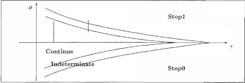
T ak e th e s e m ip l a n e (r, �J-), M > 0 ( i n ver s e of var i a n ce x m e a n ) . Divide the plane into three decision regions: a Continue re g i o n , a StopO r e g i o n and a Stopl re­ g i o n . The p o s t e r i o r d e n s it y a f t e r m eas u r e m en t Xn i s Nn, r e pre s e n t e d by a point in the s e m i -p la n e ( T, J.t). The plan i s : check whether the posterior Nn is in C o n ­ tinue, StopO or Stopl, and r e s pec ti v e l y take a new me a s ur e m e n t , stop a n d pick d0, st o p and pick d1. The p la n is d e t e r m i n e d by the d e ci s io n r e gi on s , which are created by d y n am i c p ro g r a m m i n g (value i t e r a t i o n al­ gorithm ) [ DeGroot, 1970], as explained in A p pe nd i x A.

4.3 PLANNING WHILE ACTING

The agent has a prior credal set defined by /J-l, �J-2 a n d z:; as measurements a re collected, the decision regions must be constructed for L. + nr, where n s ta r t s fr o m ze r o .

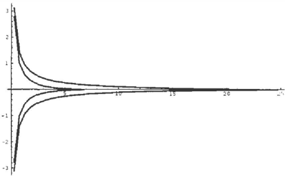
Th e wh o l e p l an is defined by the upper and lower boundaries of the Continue region. The value it­ er a ti o n algorithm essentially brackets this region and c o n v e r g e s to the correct boundary, but every it e rati o n r e q u i r e s m o r e e ff o r t t h a n t h e p r e v i o u s iteration. Given any finite amount o f c o m p u t a ti o n , t he a g ent , B a y e si a n or Quasi-Bayesian, has a c h ar t similar to F i g ur e 3 [ De­ Gr o o t , 1970]. Th ere is an Indeterminate r e g i on , yet to be e x p l o r e d . The agent can shrink the s i z e of t h e Indeterminate region at high computational cost, as discussed in Appendix A. A real agent has a region of computational indeterminacy: because a fi n i t e amount of effort is available, not all plans can be evaluated.

We have returned to the Archers Fable. We have the p l a n e ( T, M), and we must hi t t h e bound a r y of t h e Con­ tinue r e g i o n .

T h e Baye s i a n archer wants to find a single curve. Any lack of precision in the p r i or models will r e q u i r e a sen­ sitivity a n a l y s is or a m e t a -a n al y s i s. This may lead the Bayesian archer to spend a vast amount of computa­ t i o n if the archer is considering a point close to the boundary between Continue and Stop regions.

The New Quasi-Bayesian archer thinks differently. The New Quasi-Bayesian agent recognizes that as s o o n as t h e re is a point in so m e r e g i o n outside the Indeter­ minate region, the w h o l e situation is characterized. If t h e credal set is inside the StopO r e g i on , then stop awl pick do; if the credal set is in s i de the Stopl region, t h en stop and p i c k d1; if the cr e d al set. i s inside t!H' Continue re g i o n , then take another observation. But if the credal s e t intersects more than o n e region, a non­ robust sit1wtion has been detected. The agent h a s ;m E-admissible a ct i o n that can be d ws e n . but rolmstw's� has failed. So the New Quasi-Bayesian archer s h r in k s the Indeterminate r e g i o n o n l y if all distributions in the c r e da l set are inside this r e g i o n .

To make this strategy co n cr e t e , consider an example. F i g ur e 3 s h o w s the f o ur decision regions. Each vertical se g m e n t represents a set of "pure" Gaussian distribu­ tions w i t h the same varianrP. ThP first hand is t }J(' p r i o r band. Since the band is i n si de the Continue r e g i o n , the agent takes a new measurement \vitlwut further c o mp u t at i o n . Now the band c r o ss e s both Con­ tinue and Stopl. The agent knows, without fu,r·thn computation, t h a t both t a k i n g a new measurement awl c h oo s i n g d1 are a d m i s s i b l e , no ma t t e r how much addi­ tional e ff o r t is spent. If an a n y t i m e decision is needed a t this point, a new observation is taken. But tlw cor­ rect a n a ly s is is that the prior imprecision has creatHl a n o n -r o b u st situation where a possible action is to continue observing.

This strategy links the computational indeterminacy of the planning algorithm to thf! rn�rlfll inclPtPnninacy of the agent., formalizing a c o n n e c t i o n between s<�arc:h e ff or t and model b u i l d i n g . There are limits to the d'­ f o r t that is worthy s p e n di n g in s e a r c h for a given h;wl of imprecision in a probability assessment. Thi" work a p p e a r s to be the first a na l y s i s of this trade-off with the tools of Quasi-Bayesian t h e or y . Some new ques­ tio ns emerge. First, what are the methods t hat de­ fine t h e agent's behavior when two decisions are mm­ p u t a bl e and admissible? Second, what are the ap­ p r o x i m a t i o n algorithms (value i t e ra t i o n in this c a se) that admit a r e l a t i o n s h i p between comp u t a t i o n a l and credal indeterminacies? Third, i s th e a pp r o x i ma t i o n a l g o r ith m biased, i.e., is it c a u s i n g t h e a g e n t to pick so m e r e g i o n s more than others? This h a ppe n s, for ('X­ ample, if th e Indeterminate region greatly extends i n t o one of the Stop regions but not i nt o the other:1·

4.4 PLANNING IN ADVANCE

An a n al y s i s of t h i s problem must take into account tlw p o s s i b i li t y that the agent pre-computes the t!Pcision r e g i o n s . In g e n e r a l , suppose the agent wants to pn;­ compute t he relevant decision regions for prior w id t h D. an d prior i n v e r s e v a r ianc e z:. So the agent must prP­ compute the r e g i o n s for allz:+nr, w h e r e n starts from zero.

The New Q u a s i -B a y e s i a n archer has simply to )!;Uar-

3 The fact that this may occur was suggested to us hv Prof. T. Seidenfed.

antee that the band of "pure" Gaussians does not fall entirely inside the Indeterminate region. This can be done in a finite number of iterations given the monotone character of the value iteration algorithm (Appendix A) and the fact that the posterior set of Gaussians has a width that decreases as .D.TI(T + nr).

For the New Quasi-Bayesian archer, the question arises as to whether or not we can determine the boundaries of the Indeterminate region without even iterating the value iteration algorithm. Of course, this must depend on the characteristics of the initial credal set. Suppose the agent starts with a given prior variance 1/L and a given prior width .D.. The following new re­ sult characterizes the situations that admit direct solu­ tions for the boundaries4. The result is even stronger than what we just required: it covers all plans where priors have width smaller than .D. and variance smaller than 1/L.

Theorem 1 If z!t(z.D.T 12) < c for T"-112 :'::: z :'::: T'- 1 1 2 , then the following decision regions completely specify the agent's behavior for I. and .D.:

Stopl J1 � max(O,U(cft)lft)

StopO J1 :::; min(O, -U( eft) I ft)

Indeterminate otherwise. 0

We can summarize the New Quasi-Bayesian strategy for generating plans:

1. Theorem 1 verifies whether the Quasi-Bayesian plan can be stored in closed-form.

4The following definitions are used: rp(s) is the standard Gaussian density and iP(s) is the standard Gaussian distri­ bution function; D(s) = ¢(s) + (1iP(s))s; U(s) is the inverse function of D(s); T1 = JCr/2)2 + (r/2)/('rrc2)- (r/2) and r" = 1/(27rc2).

1. If not, then the value iteration algorithm shrinks the Indeterminate region. When the Indeter­ minate region is smaller than .D. T I T for every T larger than I., the decision regions are defined.

We now look at a situation that occurs in practice and leads to increased savings within the New Quasi­ Bayesian framework. Suppose the agent has to provide plans for a variety of values of the cost of observations c. A situation where this happens is illustrated in the next section. Here we consider the c o st s c1 to belong to a finite set of values { c 1 , c2 , . . . , ern}.

The boundaries of the Indeterminate region must be generated for each one of the costs c;. T he following result is useful:

Theorem 2 If the conditions of Theorem 1 em� sat­ isfied for a value c*, they are satisfied for· a val'IIJ� c larger than c*. 0

At first, the New Quasi-Bayesian identifies a value of Ci that admits closed-form plans using Theorem 1; for larger values of ci the plans can be directly stored. For other values of Ci, the agent must construct bound­ aries for the decision regions by iteration. The value iteration algorithm must shrink the Indeterminate region until it is smaller than the width of the credal set. Again, as the problem became more involved, tlw savings in the New Quasi-Bayesian scheme increased when compared to the Bayesian prescription.

4.5 EVALUATING THE SOLUTION IN A REAL PROBLEM

Consider the construction of a robotic probe for classi­ fication of material based on acoustic signals [Krotkov and Klatzky, 1995]. The taks is for a robot to d<'­ cide whether a material belongs to one of two dass<�s based on the tangent of the angle of internal hictioll, tan¢, which is captured from acoustic analysis of im­ pact sounds. This is equivalent to deciding whether a variable f) (linearly related to tan¢) is larger or smaller than zero. The losses are given by table 1. Tlw mbot

is used for a variety of tasks; when the robot is as­ signed to a task, a cost for robot operation is assigned based on the number of waiting tasks in a queue. So the act of striking a material costs a quantity c; which belongs to a finite set of possible costs { c1, c2, . . . , em}, corresponding to the size of the queue. Once the task is initiated with a cost c;, the cost remains fixed during that task.

Suppose we want to distinguish metals with tan¢ above -11 (aluminum has tan¢ of approximately -2) from non-metallic materials with tan¢ below -11 (plas­ tic has tan¢ of approximately -20). We translate these values so that f) is zero when tan¢ is -11; now we de­ cide whether f) is larger or smaller than zero. Experi­ ments suggest a Gaussian model for the measurements: X; ,... N(x;; 8, r), with r = 1 [Krotkov and Klatzky, 1995].

Very sparse knowledge about 8 must be translated into a belief model. Trying to model this with a single prior leads to a number of arbitrary choices. Instead, take the prior model to be a Quasi-Bayesian set No with variance 1/T_ = 4, JL1 = -5, fJ2 = 5 (so that 6. = 10).

The last element to be specified is the cost of an ob­ servation. We consider a vector of possible costs, de­ pending on the state of the robot, and assume a linear relation: c; = ci, i E {1, _ _ . , 10}, when'! i is the num­ ber of tasks in the robot queue, including the one the robot is operating on. We must define c, the cost of an observation when no task is waiting. Instead of fixing a value of c arbitrarily, we build some intuition by ask­ ing the question: If we had just a single Gaussian prior defined by mean /-l, JL > 0, and variance 1/r_, and the right to take a single observation, what would we do? For fJ larger than a certain value 1--l', we would rather take d1 than pay c. So our choice of J-.L' encodes the value of c. T h e value c such that p/ is the boundary of the Continue region for r_ is:

In our particular example, we took fJ1 = 4, signifying that, unless we believed strongly that e > 0, we would prefer to take a new observation. In other words, we regard the cost c to be relatively small. The use of the previous equation with r_ = 0.25, 1--l' = 8 and r = 1 gives us c = 7.88 x 10-3. We round that and adopt c = 0.01 to represent an appropriate cost for the mea­ surements, so we have c; E {0.01, 0.02, . . . , 0.1 }.

First we search for closed-form solutions. Theorems 1 and 2 indicate that values of c > 0.081 lead to closed-form plans. We must only obtain plans for c; E {0.01, 0.02, ... , 0.08} (for the results in this sec­ tion, we used a symbolic package which we are making publicly available; see Appendix B for details).

For c; = 0.07, the Indeterminate region is shrunk sufficiently by a single iteration of the value iteration

algorithm (i.e., reaching p� and fJn. For c; = 0.03, two iterations of the algorithm are necessary to oh­ tain the decision regions. Below this value, the com­ putational effort involved in computing the decision regions is rather large. Instead of sacrificing time to compute these plans, we use "lumped" observations. When ci E {0.01, 0.02}, we take two observations at a time; the "lumped" observation is the average of tlw two observations and has precision 0.5. The bottom of Figure 4 shows the resulting decision regions for Ci = 0.02.

The plans have a satisficing character in which the�y are admissible in the light of prior beliefs, yet they atT o pe n to challenge: during operation, the robustm?ss of any decision may be compared to other admissible decisions and better courses of action can be leamc�d or experimented. There is no need to obtain a si n ­ gle "best" plan and then conduct se n s it ivi t y analysis on it: the overall strategy already encodes a.ll rolmst and non-robust situations the agent may face. Since' the credal set and the decision regions are available to the agent, robustness questions can be dealt with in a straightforward manner. From this simple examph� W(' notice how the questions of model precision, computa­ tional effort and robustness can be all tied together in the New Quasi-Bayesian framework.

5 CONCLUSION

We have proposed a new approach to decision-makiug with Quasi-Bayesian models. Quasi-Ba.y,�siall tlwory maintains that a convex set of probability distributions captures the beliefs of an agent. The t h e o r y docs uot. specify how two decisions are to be c o m p a n� d wlwu they are both admissible. This has l e d to a gn�at. deal of anxiety among researchers, who have proposrd ad d i­ tional constraints to allow any comparison to be made�. We depart in a somewhat radical way from this tradi­ tion: instead we propose that any admissible decision can be chosen, but that robustness must be monit.on�d by the agent. A non-robust decision must be refined if possible. If there is no time for refinement, a default

admissible action is used.

We have demonstrated this approach to decision­ making in a problem of planning to observe, where prior beliefs are captured by a set of Gaussian distributions. We demonstrate how to monitor robustness and how to choose E-admissible actions. Our proposal can be extended to the class of planning to observe problems with multivariate data or with general distributions and conjugate priors (for example, beta priors with binomial observations [Lindley and Barnett, 1965]). Further research is needed to extend these ideas to other, more general decision problems.

The plan generation algorithm here developed is, to the best of our knowledge, the first example of a sit­ uation where Quasi-Bayesian theory helps to reduce the complexity of g e n e r a t i n g a decision plan. This is due to our focus on the robustness, rather than the optimality, of a solution. We expect this approach to shed light on the relationship between rationality re­ quirements and computational effort. Note that we do not suggest that models should be imprecise to facil­ itate search. We do suggest that the use of a model should be compatible with its precision. The Bayesian strategy sometimes seems excessive in that it forces a precise model into a problem and then demands op­ timality or meta-analysis with respect to that model. A Quasi-Bayesian approach that focuses on robustness and computational effort can offer a new perspective for decision making.

The theory developed above admits a different, pos­ sibly fruitful, interpretation. Suppose an agent has a Quasi-Bayesian model and the agent is not interested in the robustness of actions; instead, the agent wishes to generate admissible actions as fast as possible. This interpretation of Quasi-Bayesian decision making (as advocated by [Good, 1983]) is that the agent has ex­ hausted preferences and can pick admissible actions arbitrarily. We demonstrated that, for t h e planning to observe problem, the agent can generate E-admissible plans faster than a Quasi-Bayesian agent could gener­ ate a "best" plan.

A THE QUASI-BAYESIAN RISK

We wish to minimize the Bayes risk for a Gaussian prior with m e a n /-1, v a r i a n c e 1/r by using a plan J. The Bayes risk is

Note that the number of observations n is also a ran­ dom variable to be averaged in the expectation. Call p(J.I, r ) the value of the Bayes risk for the Bayesian best plan.

Dynamic programming applied to this minimization problem leads to a value iteration algorithm [DeGroot, 1970]. Very briefly, the algorithm assumes that two initial guesses of p are given: iJb(f..L, T ) and p�(f..L, T ) , such that p0(f..L, T) � p(J.I, r) � p� ( f..L , r) .

Two iterations compose the algorithm, one for p; J (/<, r) and another for p� (11, r ) . Each iteration is (prime� arc dropped since the next expression can be used both for Po and iJ�):

The following fact is guaranteed for any 'i [DeGroot., 1970] (intuitively, the algorithm "sandwiches" p(JL, T)):

The result is:

• if p;(fl, r) = Po( fJ , r) and fl 2 0, then (T, 11) is in a Stopl region;
• if p;(/-1, r ) = po(f..L, r ) and p, � 0, then ( r, JL) is iu a StopO region;
• if p;' (f..L, T ) =1p0 (p, T ) , then ( r, p,) is in the Con­ tinue region.

This produces the decision regions, with the Continue region between the StopO and Stopl regions. Intu­ itively, the algorithm "sandwiches" the Indetermi­ nate region.

In order to start value iteration, the following choices are adequate: Po(f..L, r ) = 0 (always smaller than p(f..L,r)), and p�(fl,T) = Po(fl,r), where Po(fl,T) = rl(?rMI). The function po(f..L, r ) is always larger than p(p, r) [ D eGroot, 1970].

B A PACKAGE FOR QUASI-BAYESIAN PLAN GENERATION

The results discussed in this paper were impk­ mented in a Mathematica™ package which is pub­ licly available through anonymous ftp. Connect to ftp.cs.cmu.edu as anonymous, go to t h e directory /afs/cs/project/lri-3/ftp/outgoing/ and get th<� file quasi-bayes. tar. Use the tar program and read tlw README file for the necessary guidance.

Acknowledgements

This research is supported in part by i\ ASA under Grant NAGW-1175. Fabio Cozman is supported ll!l­ der a scholarship from CNPq, Brazil.

We thank Prof. T. Seidenfeld and L. Chrisman for reading an earlier draft and suggesting substantial im­ provements to this work.

References

• [Berger, 1985] J. 0. Berger. Statistical Decision The­ ory and Bayesian Analysis. Springer-Verlag, 1985.
• [Breese and Fertig, 1991) J. S. Breese and K. W. Fer­ tig. Decision making with interval influence dia­ grams. In P. P. Bonissone, M. Henr i o n, L. N. Kana!, and J. F. Lemmer, e d i t o rs , Uncertainty in Artifi­ cial Intelligence 6, pages 467-4 78. Elsevier Science, North-Holland, 1991.
• [Chrisman, 1995] L. Chrisman. Incremental condi­ tioning of lower a n d upper probabilities. Interna­ tional Journal of Approximate Reasoning, 13(1):125, 1995.
• [DeGroot, 1970] M. DeGroot. Optimal Statistical De­ cisions. McGraw-Hill, New York, 1970.
• [Fertig and Breese, 1990) K. W. Fertig and J. S. Breese. Interval influence d i a g r a m s . In M. Hen­ rion, R. D. Shachter, L. N. Kana!, and J. F. L e m ­ mer, editors, Uncertainty in Artificial Intelligence 5, pages 149-161. Elsevier Science Publishers, North­ Holland, 1990.
• [Fine, 1988] T. L. Fine. Lower probability models for uncertainty and nondeterministic processes. Journal of Statistical Planning and Inference, 20:389-411, 1988.
• [Giron an d Rios, 1980] F. J. Giron and S. Rios. Quasi­ Bayesian behaviour: A more realistic approach to d ec isio n making? In J. M. Bernardo, J. H. DeGroot, D. V. Lindley, and A. F. M. Smith, editors, Bayesian Statistics, pages 17-38. University Press, Valencia, Spain, 1980.
• [Good, 1983] I. J. G o o d . Good Thinking: The Founda­ tions of Probability and its Applications. University of Minnesota Press, Minneapolis, 1983.
• [H. E. Kyburg J r . , 1987] H. E. Kyburg Jr. Bayesian and non-Bayesian evidential updating. Artificial In­ telligence, 31 :271-293, 1987.
• [Halpern and Fagin, 1992] J. Y. H alp e r n and R. Fa­ gin. Two views of belief: Belief as generalized prob­ ability and belief as evidence. Artificial Intelligence, 54:275-317, 1992.
• [Beckerman and Jimison, 1989] D. Beckerman and H. Jimison. A Bayesian perspective on confidence. In L. N. Kana!, T. S. Levitt, and J. F. Lem­ m er , editors, Uncertainty in Artificial Intelligence 3, pages 149-160. Elsevier Science Publishers, No r th ­ Holland, 1989.
• [Horvitz, 1989] E. J. Horvitz. Reasoning about be­ liefs and actions under computational resource con­ traints. In L. N. Kana!, T. S. Levitt, and J. F. Lemmer, editors, Uncertainty in Artificial Intelli­ gence 3, pages 301-324. Elsevier Science Publishers, North-Holland, 1989.
• [Krotkov and Klatzky, 1 995] E. Krotkov and R. Klatzky. Robotic perception of material: Ex­ periments with shape-invariant acoustic measures of
• material type. Fourth International Syrnposi·11.m. on Experimental Robotics (ISER95), 1995.
• [Levi, 1980] I. Levi. The Enterprise of Knowledye. The MIT Press, Cambridge, Massachusetts, 1980.
• [Lindley and Barnett, 1965] D. Lindley and B. N. Barnett. Sequential sampling: Two decision prob­ lems with linear losses for binomial and n o r m a l ran­ dom variables. Biometrika, 52:507-532, 1965.
• [Matheson, 1968) J. E. Mat h e s o n . The economic valu<' of analysis and computation. IEEE T ra n s . on Sy8tems Science and Cybernetics, SSC-4(3) :325--332, September 1968.
• [Ruspini, 1987] E. H. Ruspini. The logical foundations o f evidential reasoning. Technical Report SRIN 408, SRI Int., 1987.
• [Russell an d Wefald, 1991] S. Russell and E. \V(,fald. Do the Right Thing. The MIT P r e s s , Cambridge�, MA, 1991.
• [Seidenfeld and Wasserman, 1993] T. Seidenfeld awl L. Wasserman. Dilation for sets of probabilities. Th(' Annals of Statistics, 21(9) : 1 139-1154, 1993.
• [Seidenfeld, 1993] T. Seidenfeld. Outline of a theory of partially ordered preferences. Philo8ophical Topir:s, 21(1) : 1 73-188, Spring 1993.
• [Shafer, 1987] G. Shafer. Probability judgment iu ar­ tificial intelligence and expert systems. Stati:;timl Science, 2(1):3-44, 1987.
• [Smith, 1961] C. A. B. Smith. Consistency in statisti­ cal inference and d e c i s i o n . Jonrnal Royal Statisbr:al Society B, 23: 1-25, 1961.
• [ Suppes, 1974) P. Suppes. The measurement of IH"lid. Jonmal Royal Statistical Society B, 2:160-191, 1974.
• [Walley, 1991] P. Walley. Statistical R e as o n i n g with Imprecise Probabilities. Ch ap m a n and Hall, N<'w York, 1991.