Real-valued All-Dimensions search: Low-overhead rapid searching over subsets of attributes

Andrew Moore

School of Computer Science Carnegie Mellon University Pittsburgh, PA 15213

Abstract

This paper is about searching the combina­ torial space of contingency tables during the inner loop of a nonlinear statistical optimiza­ tion. Examples of this operation in various data analytic communities include search­ ing for nonlinear combinations of attributes that contribute significantly to a regression (Statistics), searching for items to include in a decision list (machine learning) and associ­ ation rule hunting (Data Mining).

This paper investigates a new, efficient ap­ proach to this class of problems, called RAD­ SEARCH (Real-valued All-Dimensions-tree Search). RADSEARCH finds the global op­ timum, and this gives us the opportunity to empirically evaluate the question: apart from algorithmic elegance what does this attention to optimality buy us?

We compare RADSEARCH with other recent successful search algorithms such as CN2, PRIM, APriori, OPUS and DenseMiner. Fi­ nally, we introduce RADREG, a new regres­ sion algorithm for learning real-valued out­ puts based on RADSEARCHing for high­ order interactions.

1 THE GENERALIZED RULE-FINDING PROBLEM

This paper is about searching the combinatorial space of contingency tables during the inner loop of a non­ linear statistical optimization. Examples of this op­ eration in various data analytic communities include searching for nonlinear combinations of attributes that contribute significantly to a regression (Statistics), searching for items to include in a decision list (ma­ chine learning) and association rule hunting (Data Mining).

Jeff Schneider

School of Computer Science Carnegie Mellon University Pittsburgh, PA 15213

This paper investigates a new approach to this class of problems, called RADSEARCH (Real-valued All­ Dimensions-tree Search). Unlike AD-trees, RAD­ SEARCH does not need to pre-build a data structure of cached statistics prior to searching, and so is prof­ itable even if only one search is needed, or if subse­ quent searches need to occur on different subsets of the records. RADSEARCH generalizes to searches in which the contingency tables may contain vectors of real-valued aggregates, permitting searches for tables and rules that (for example) maximize the mean of a real-value, minimize a value's variance or give the highest variance explained.

Given a dataset and a rule size: k, we define the gen­ eralized rule-finding problem as finding:

• A rule ru is a conjunctive propositional formula ( q :'0 k):

• matchers(ru) is the set of row numbers in which the rule ru is satisfied.
• statvec; is a user defined vector dependent on the attribute values of row number i. These will be summed for all rows matching the rule. For example, if one element of statvec; is 1 for all rows, the effect of summing over all those that match the rule is to count the number of records matching the rule. We use sumstats[j] to refer to I:; statvec; [j].
• score is a user-specified function that operates on sums of statvecs. The goal is to find the rule with the maximum value of score

一

Here are four instances of generalized rule finding:

1. Search for the rule in which the largest fraction of records have agegroup = middle. To do this, define

statveci = (1, 1) if ith row is middle-aged statveci = ( 1, 0) otherwise

Summing the statvecs of the matching records results in a two element vector where the zeroth element counts the number of records matching the rule and the first element counts the number containing the desired value of agegroup. Then maximize the following score function:

where nmatch is the number of rows matching the rule and nmiddle is the number of middle-aged rows matching the rule.

1. Search for the rule in which the age-group (one of young, middle and old) is most predictable. To do this, define

statveci = (1, 0, 0) if i th row is young

statveci = (0, 1, 0) if ith row is middle-aged

statveci = (0, 0, 1)

if i th row is old

Then maximize the negative entropy of the dis­ tribution implied by the counts (this criterion is used by [Clark and Niblett, 1989], for example):

1. Search for subgroups in which mean income is high: statveci = (1, in;) where in; is the value of the real-valued attribute income within the ith record. Then score(nmatch, 2:: in;) = 2:: in;/ nmatch ·
2. Search for subgroups in which income is pre­ dictable: statveci = (1, in;, in;2) and

which is the negative mean squared error of predicting income by its mean among the rows matching ru.

Usually the score function is modified to ensure signif­ icance. This can be done simply by giving a score of -oo to any rule that matches fewer than some threshold, nsupport, of rows [Agrawal et al., 1996, Mannila and Toivonen, 1996]. It is also possible to use more traditional tests of significance as part or all of the rule evaluation [Duda and Hart, 1973]. We emphasize that the above four are only examples of a much larger space of useful generalized rule searches.

1.1 RELATED WORK

Rule learning and decision lists are a popular ap­ proach in machine learning, pioneered by [Rivest, 1987, Michalski et al., 1986, Clark and Niblett, 1989]. Generally, they search for the kind of conjunction-of­ literals rules described above, concatenating them into chained if-then-elseif-... statements. For classification, this paper gives very similar algorithms, except that we search a much wider space of possible rules and thus avoid the (imagined or real) pitfalls of heuristic search. For regression (learning real-valued outputs) lists have also been investigated, including a recent al­ gorithm called PRIM [Friedman, 1998] which learns a list in which outputs are numbers. In this paper we allow a much more aggressive search for components of such rules.

A form of Rule-learning has also recently gained pop­ ularity in the literature of data-mining [Agrawal et al., 1996, Srikant and Agrawal, 1996, Mannila and Toivonen, 1996]. These ingenious algorithms restrict themselves to rules with positive literals (e.g. you cannot learn a rule "if you buy bread and no but­ ter then you'll buy margarine") but in the presence of very sparse binary data can find optimal rules ef­ ficiently, sometimes with only one pass through the data. In this paper we try to avoid the restriction to positive literals and we give algorithms that are efficient even on dense data (i.e. non-sparse data) and high-arity attributes. We also allow searching for rules with more general statistics than counts. The price is increased expense compared with sparse posi­ tive literal learning. OPUS [Webb, 1995, Webb, 2000, Webb, 2001], which we compare against, addresses a similar problem.

For general database queries involving additive aggre­ gates (sums of statvecs above) there has been excit­ ing progress around structures called datacubes [Hari­ narayan et al., 1996]-these will be described and used in this paper.

2 THE RADSEARCH ALGORITHM

2.1 NAIVE RULE SEARCH

• For each rule ru of length � k do
• sumstatsru = I: iematchers(ru) statveci
• s cor e ru = score ( sumstatsru )
• Return the best-scoring rule.

If there are R records then each execution of step 1 requires at least O(R) time (approximately O(R log q) for a q-attribute rule, because on average log q tests are needed to see if the rule matches each row).

For brevity throughout this paper we assume binary­ valued input attributes. In general the same analytical conclusions will follow for other arities. The empiri­ cal results will contain many datasets with multiple­ valued (sometime hundred-valued) attributes. Assum­ ing M attributes in atts then the number of sets of attributes to consider is

But for each set of k attributes there are 2k rules to consider, each needing a pass through the dataset. In total then, there will be at least O(R2k ( �)) work for the naive algorithm.

2.2 NOT-SO-NAIVE METHODS

It is easy to reduce cost by a factor exponential in k. Search over all datacubes involving k or fewer of the attributes.

Assuming binary attributes, a q-dimensional dat­ acube [Harinarayan et al., 1996] for attributes (att1, att2 .. attq), denoted DC(att1att2 .. attq), is a q di­ mensional 2 x 2 x ... x 2 array in which each cell con­ tains a sumstats vector. Let i1 .. . iq be indices into the array, where each index is either 0 or 1. Then the cell corresponding to indexes i1 .. . iq contains the sumstats vector for the rule ( att1 = i1, at� = i2, . .. att q = iq)·

Given any subset of q attributes, a datacube can be obtained in time O(qR + 2 q ) by one pass through the dataset in which the only piece of work done for each record is to decide which cell to add its statvec to. Thus for the cost of one pass we build the sumstats for 2q rules. The entire search cost is now only

The 2k term remains, simply for initializing the dat­ acube. It is now added to the R term instead of mul­ tiplying R. Usually 2k << R.

2.3 RADSEARCH: FASTER NOT-SO-NAIVE

Our next improvement will reduce the cost of the con­ struction of a level-q datacube from O(R + 2q) down to O(R>.q + 2q), with .\ (described below) much less than 1. Previously, each of the 0 ( ( �)) datacubes we searched over were created independently. Now we will maintain two data structures throughout the search that together will usually allow the generation of the "current" datacube to exploit a great deal of the work by the "previous" datacube. These two structures are:

• A Row Tree, to be described shortly, which sparsely indexes rows specific to the current dat­ acube in such a way that the set of changes needed to move to the "next" datacube is small.
• A modified AD-tree [Moore and Lee, 1998], which stores, in a highly compressed form, information sufficient to recreate all k -1 dimensional dat­ acubes we encounter during the search. This gradually grows as the search progresses.

2.3.1 ROW-TREES

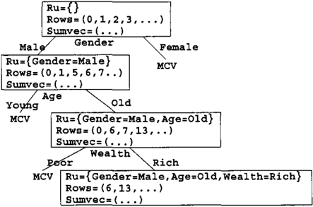
A Row-tree is a simple data structure defined by a set of attributes and a set of rows. Figure 1 shows a row tree for three attributes. Every node corresponds to a rule and contains a list of all rows that match the rule and the sumvec (sum of statvecs) for all rows that match that rule.

The root node is the empty rule, matching all records. The ith child of a node N at depth d corresponds to a specialization of N's rule in which the literal attd = vali is appended.

Row-trees have another important property. Every non-leaf node fails to store information about the child with the most common value (MCV) of the split at­ tribute. Only a tag denoting the MCV is stored.

Before discussing how we use rowtrees we describe the compressibility .\ of the database.

Definition 1. Compressibility(.\) is the average frac­ tion of rows that survive in a rowtree from one level to the next when MCV values are thrown out.

Low compressibility values are beneficial and occur in two ways:

1. Data with sparse attributes have low .\ values. Indeed if all attributes are independent and have

= 12:1

probability p of being 1 then the dataset has .\ = min(p, 1p).

1. More importantly than sparseness, correlations between pair, triplets up to k-tuplets of attributes help make good compressibility. If att1 is usually the same as at� then the MCV of att2 will be most of the records in any part of a rowtree where att1 has been instantiated as a parent.

Overall in real-world datasets we have seen compress­ ibility values .\ ranging from w-3 to w-1 but have never seen compressibility worse than 10- 1 .

Notice that the total space to store a k-attribute rowtree, including all lists of row numbers is

2.3.2 BUILDING A DATACUBE FROM A ROWTREE AND ADTREE

Assume we have a row-tree corresponding to a set of attributes (att1att2 .. attk)· We are now going to see how we can use it to to create a datacube for those at­ tributes, in time independent of R ( number of records ) and M ( total number of attributes in the database). It would be wonderful if the datacube could be con­ structed entirely from the rowtree but sadly too much information has been lost. Instead we will use a shal­ low AD-tree-like structure [Moore and Lee, 1998].

An AD-tree is a data-structure that allows us to rapidly find datacubes by caching. Originally they were only used to cache counts of rows-the extension introduced here to cache arbitrary sums of statvecs is relatively simple and will not be discussed fur­ ther. If we are searching for rules up to length k we only build an AD-tree capable of reproducing dat­ acubes of dimension k-1 or less. Usually the cost of building such an AD-tree would be R(M + >.( �) + >. 2 (�) . . . >. k - 2 V:: 1 )) but in this case it can be built for free during the rowtree search to be described shortly.

A more serious AD-tree issue is the memory require­ ment. By using MCVs astutely, it manages to only store ( k�1 ) sumstats. The fact that we are using ( k�1 ) instead of ( 'i[) usually brings down memory use by an order of magnitude.

Now, let us consider how to build a datacube for at­ tributes (a1 ... ak) using a rowtree for (a1 .. ak) and a depth k 1 AD-tree. We will need to use an extra piece of notation: Let DC(a1 ... aq lru) be the datacube for ( att1 .. attq) built only from those records matching ru.

Returns DC(att1 .. attq1RT.ru), using an ADtree AD and using a rowtree RT built for ( att1 att2 .. attq).

Define RT.ru to be the rule correspond­ ing to the row tree node RT. As an ex­ ample, in Figure 1 the topmost node has RT.ru = {} (the empty rule). The bottom node has RT.ru = {Gender = Male, Age = Old, Wealth = Rich}.

1. If attribute-list is empty (q = 0), return the 0dimensional datacube with a single cell containing RT's sumstats.
2. Let LCV be the least common value of att1 among records matching RT.ru and let MCV be the most common value of att1 among records matching RT.ru. The values of LCV and MCV are im­ mediately available from RT.
3. Let DCubeLCV = Bui1dDC ((att2 .. attq) , AD , RT .child[LCV])

Note that RT.child[LCV] is non-null. Also note that in the non-binary­ attribute case, there is one call for ev­ ery value of the attribute except for the MCV.

This operation sets DCubeLCV = DC(att2 .. attqiRT.ru II att1 = LCV). Thus it is a q -1 dimensional datacube for attributes ( att2 .. attq) over all records that match both the rule RT.ru and in which att1 = LCV.

Next we will build DCubeMCV but we cannot use the same kind of recursive call as we used for DCubeLCV because RT.child[MCV], which would be needed

for the call, is NULL. So instead, in the following two steps, we will obtain it in­ directly.

1. Let DCubeAll = DC (at� .. att q i RT . ru ) obtained from AD.
2. Let DCubeMCV = DC( atf:l .. attq IRT.ru A att1 = MCV) computed by the cellwise subtraction of all cells in DCubeLCV from their corresponding cells in DCubeAll
3. We now have two (qI)-dimensional datacubes: one for attributes at� .. attq in the case where att1 = 0 and one for the same attributes in the case where att1 = 1. These two datacubes con­ tain all the values needed for the q-dimensional datacube defined by att1 .. attq, which we construct and return.

Step 3 is a recursive call. In total there will be k levels of recursive calls starting from the top level call BuildDC((att1 ... attk) ,AD,RootRT) called with an empty rule.

At all levels of recursion, Step 4 strains the limit of what a k - 1-depth AD-tree can construct because the total number of attributes mentioned in (att2 .. attq) plus the total number of attributes in the condition ru is k1 at all levels of recursion. AD-trees can produce a datacube of q attributes in time 0(2q) and a condi­ tional datacube of r attributes subject to a conditional of s literals in time 2r+s. An AD-tree of depth k - 1 can construct its answer, however, only if r + s :-:; k-1.

Step 5 is the same idea that underpins AD-trees: if you have the "conditional" datacube for one binary condi­ tion and the "marginal" datacube then the conditional for the other condition can be obtained by subtraction.

Surprisingly, despite all the recursion, the total work of building the k-dimensional datacube from RT and AD is only 0(2k), independent of M and R. Since the datacube size is 0(2k) we could not hope to do better.

2.3.3 SEARCHING THE SPACE OF ROWTREES

We have now seen how to use a depth k-1 AD-tree and a depth k rowtree to compute the datacube for a spe­ cific set of attributes mentioned in a rowtree. In this section we return to the top-level problem of searching through all sets of attributes of size k or less.

Naively, we could search through all rowtrees of depth k or less, and for each rowtree build the datacube for the given set of attributes and for each rule in each datacube compute the score of the sumstats vector. But that would gain us nothing, since each rowtree would require O(R) time to construct, where R is the number of records.

Instead we can move between rowtrees without need­ ing to fully construct a new rowtree at each step, but instead tweak the previous rowtree.

A typical move to the "next" rowtree usually involves merely changing the leaf node (e.g. ( att1 = age, att:J = gender, att3 = wealth) changing to ( att1 = age, att:J = gender, att3 = education)). Occasionally we need to change the second node from the bottom and very oc­ casionally the third, and so on. Some reflection shows us that:

• ( �) of the steps involve altering only the bottom (kth) level. Each such step will require an itera­ tion through all the rows mentioned in the k -1 'th level. There are Ak-1 R such rows. So the work for level-k-altering rowtrees will be Ak-1 R(�)
• Similarly, the total work on level-q-altering rowtrees (for q = 1, 2 . . k-1) will be Aq-1 R(�). For example, for top level ( q= 1) changes we will do A0R('Y) = RM work, as expected.

The above bullets neglect the fact that for each set of attributes we must not only find the matching rows and sumstats, but must also execute the above dat­ acube construction procedure. This negligence is rea­ sonable for large R.

The total work over all pruned rowtrees is thus:

Usually the rightmost term will dominate, making the work done O(Ak-1 R(�)), a factor of (1/A)k-1 times faster than the not-so-naive method. Since A is typi­ cally w-3 to w-1 this is considerable.

Sometimes (e.g. if A< k/M) the rightmost term won't dominate. Then for fixed A the cost is a lower power of M than the original method-a more impressive saving. Notice that the critical driver of the search is AM: the difficulty of search is not simply dependent on the number of attributes. A highly compressible 1000-attribute dataset might be easier to search than a weakly compressible 50-attribute dataset.

RADSEARCH is guaranteed to find the optimal rule of length k or less. This is because it searches every cell of every datacube of dimension k or less.

All the analysis has assumed binary attributes. This was for ease of exposition and brevity. For higher arity attributes the worst case is worse than for binary vari­ ables, but typical empirical performance is generally

--

-;

Dataset/Output /Task	M	R	K	NSN sees	RAD sees	Speed Up
adul tjag�/mean	15	48,842	5	79	23	3
. vbirthjslhtnfent	97	9,672	3	496	4	124
conn4fscore/mean	48	67,557	3	343	16	21
covtype/classfent	38	150,000	3	595	6	99
sdss/objfmean	24	3 Mill	4	40K	436	93
kddcupfclass/ent	42	4 Mill	5	?	581	?
reuters/inc/ent	1032	10,072	3	?	8590	?

Table 1: Search times (seconds) for various datasets on a 1.7 GHz Linux workstation with 1 Gig of RAM (though no run required more than 200 megabytes). The mean task is to find a rule of size k or less that maximizes the mean output subject to matching nsupport = 50 records. The ent tries to find a rule with the lowest output entropy, again with nsupport = 50. The first four results were run for the largest k that took NSN (Not-so-naive) less than 600 seconds. We estimate that NSN would have taken at least a week for the KDDCUP dataset and reuters, though notice that the reuters dataset is one in which positive literals are typically the only ones used in most applications, and conventional sparse data structures or frequent sets would be equal or superior to RADSEARCH.

unaffected, primarily because the datacubes become sparser as the arity increases. This issue has been dis­ cussed in detail in [Moore and Lee, 1998] in the context of the combinatorics of AD-tree memory costs.

In the remainder of the paper we ask

• What are the empirical computational savings of RADSEARCH?
• Empirically, does the ability to find the optimal rule buy us anything compared with a heuristic hill-climbing rule finder?
• Is RADSEARCH useful within larger algorithms such as decision-list search?

3 EMPIRICAL SPEED TESTS

Table 1 shows wall clock timings of Not-so-Naive ver­ sus RADSEARCH on a variety of datasets described in Table 2.

3.1 COMPARISON AGAINST OPUS

In this section we compare RADSEARCH with a well-known and very successful algorithm called OPUS [Webb, 1995, Webb, 2000, Webb, 2001] which has already been demonstrated to clearly outper­ form earlier association rule algorithms such as APri­ ori [Agrawal et al., 1996] on dense data. Like RAD­ SEARCH, OPUS finds the optimal rule up to a user­ selected size. However there are differences in the goals

Table 2: Datasets used

adult	UCI census data, donated by Kohavi
vbirth	Tracking events during pregnancy. At- tributes mostly sparse.
connect4	UCI Connect 4 database of 8-ply connect4 positions. The score attribute is the value of the position (-1,0 or +1). By J. Tromp.
covtype	UCI KDD archive Forest cover type data do- nated by J. Blackard et al.
sdss	A segment of attributes from the Sloan Digi- tal Sky Survey. Predicting Galaxy class num- ber from image and spectral features.
reuters	Each record is a document and each attribute a word: the set of non-stoplist words in over 100 documents were used.
kdd99	UCI KDD "Network intrusion" database, with 42 attributes and 4.8 million records.

of the approaches which must be taken into account when comparing. OPUS is optimized for a class of rule-learning criteria in which pruning can be used to decrease the search space. In the examples below in which OPUS does well, the pruning manages to find optimal rules (or the optimal set of n rules) without mindlessly considering all possible rules. This is a clear superiority of OPUS. In cases where there is lit­ tle opportunity for pruning, or where many rules are requested, RADSEARCH is preferable.

Table 3 compares RADSEARCH versus a commer­ cially available implementation of OPUS on rule­ finding with categorical outputs (we gratefully ac­ knowledge Geoff Webb's permission to run these tests). OPUS does very well with large support, be­ cause it can prune much more aggressively than RAD­ SEARCH. RADSEARCH prefers small support be­ cause it can find excellent rules much more quickly than OPUS which then allow RADSEARCH's primi­ tive pruning capabilities to work.

In [Webb, 2001] a new version of OPUS is introduced that maximizes criteria for real-valued outputs. This software is not publicly available and does not im­ plement the real-valued criteria we use here. How­ ever, for the purposes of comparison we implemented OPUS's principal real-valued criterion called Impact. Impact(r) = nr(Jlr Jlg) where nr is the number of records matching the rule, Jlr is the mean output among records matching the rule, and Jlg is the global mean average of outputs. Table 4 compares RAD­ SEARCH against OPUS on the task of finding the 1000-top rules for the two largest datasets reported in [Webb, 2001]. In one case there is at least a 500fold speedup, in the other case no significant speedup.

Why RADSEARCH? OPUS is a powerful method that sometimes dramatically outperforms RAD­ SEARCH and is sometimes dramatically outperformed

dataset	support	find best n rules	RAD Search seconds	OPUS seconds
covtype (R=581,012)	R/10	1	626	65 115 260 683
	R/10	10	626
	R/10	100	626
	R/10	1000	740
	R/10	10000	769	3104
	R/10	100000	880	> 43200
	R/100	1	1571	344
	R/100	10	1570	415
	R/100	100	1571	557
	R/100	1000	1605	1038
	R/100	10000	1619	4200
	R/100	100000	1656	> 43200
	R/1000	1	83	583
	R/10000	1	17	692
connect4 (R=67,557)	R710	1	299	25
	R/100	1	50	88
	R/1000	1	3	162
kdd99 (R=	R/10	1	648	1068
	R/100	1	156	1653
4.9 X 106)	R/1000	1	144	1520
	R/100	1000	661	4073
	R/100	100000	1134	> 43200

Table 3: Each experiment maximized the main OPUS criterion: st rength. Consider a rule r, and let nr be the number of records matching r. Let v be the most common output value among records matching r, and let nv be the number of records with output v that also match r. Strength is nv f nr and we search for the N rules with highest strength. OPUS prunes parts of the search space that contain only rules that cannot be better than the weakest of the N rules discovered so far. RADSEARCH was allowed to prune in the same way, but due to its reliance on a search over contin­ gency tables, it can only prune a contingency table if all rules in the table are prunable. Both methods searched for rules up to length 5 and neither used more than 400 MB of memory.

	OPUS on a 800 MHz machine	RADSEARCH on a 1.7 GHz machine
covtype/ elevation	17 hours	45 sees
ipums/ inctot	12 mins	5 mins

Table 4: Comparing RADSEARCH versus real-valued OPUS.

by RADSEARCH. How should we choose between them? One choice point is generality: RADSEARCH can search using any criterion. The criteria we use in the later algorithms in the paper were chosen for their statistical meaning within an inner loop of a larger statistical computation. We tentatively believe that few of these criteria would enable significant prun­ ing within OPUS. Another choice point is specificity: RADSEARCH can efficiently perform searches for 1in-a-1000 subsets of the records. There are many ap­ plications (e.g. [Wong et al., 2002]) where results from such searches are useful and statistically meaningful.

But there are other choice points (for example, list­ ing out a small selection of highly-supported rules to a user) where we believe OPUS dominates RAD­ SEARCH. We hope, in future work, to develop algo­ rithms that combine the strengths of OPUS and RAD­ SEARCH.

Finally, [Bayardo et al., 2000] describes an algorithm very similar to OPUS in most respects except that in­ stead of limiting search to rules of a maximum length, they introduce a new pruning criterion that disallows rules for which some subset of the conditions in the rule give less than a threshold amount of improvement over a simpler rule. [Bayardo et al., 2000] reports re­ sults on the connect4 database, when searching for rules with a high proportion of drawn games. With a support of 644 records and using their rule-pruning criterion, their search appears to be reported to take about 1 hour on a 400 MHz machine, and the best rule matches a set of records in which 20% are draws. RADSEARCH takes 47 seconds on a 1.7 GHz machine to enumerate all rules of length 4 or less that match at least 644 records, and its best rule scores 30.3%. This test does not, however, allow us to directly decide whether the increased speed and accuracy of RAD­ SEARCH is due to the choice of algorithm or the choice of pruning criterion.

4 HILL CLIMBING

Why not forget optimality and use heuristic search to find a good, if not optimal, rule? This reason­ able heuristic has been used to good effect in sev­ eral rule and decision-list induction algorithms such as CN2 [Clark and Niblett, 1989] and PRIM [Friedman, 1998] and stepwise regression analysis such as [Madala and Ivakhnenko, 1994]. Hill climbing is simple:

Let ru 1 = best rule of size 1 (call it att1 = vah).

Let ru2 = best rule of the form ru 1 1\ att2 = val2·

Let ruk = best rule of the form ruk-1 1\ attk = valk.

--;

Then use ruk as the approximate argmax of Equa­ tion 1.

In subsequent experiments we will ask "when search­ ing over rules as an inner loop of a classification or re­ gression, does exhaustive search buy us any accuracy compared with hill-climbing?"

5 DECISION LISTS

Decision lists are one, but by no means the only, ap­ plication of rule searching. An example, learned by RADSEARCH, is shown in Table 5. It is constructed simply:

1. Find the rule ru for which the output attribute, restricted to rows matching the rule, has lowest entropy, subject to matching at least support rows. (Other criteria are also used).
2. Add rule => output = value to the list, where value is the most common output value in the above lowest entropy distribution.
3. Remove the matching rows from consideration.
4. Loop: Unless there are fewer than "support" rows left, Return to 1 using the remaining rows.

When the output is real-valued we can learn a deci­ sion list called a regression list by searching for rules that accurately predict the output. One way [Fried­ man, 1998] is to keep searching for rules that maxi­ mize the output (Table 6). As the matching rows are removed, the remaining dataset has a lower mean and the predictions for consecutive decision list rules tend to decrease.

Does exhaustive search beat hill-climbing? We took 194 learning problems from four datasets in which we systematically tried to learn each attribute from all the other attributes in its dataset. Table 7 indicates that in 32 or these 194 tests RADSEARCH significantly improved prediction accuracy. It never significantly reduced accuracy.

ROC curves for the classifiers learned by RAD­ SEARCH are almost always substantially better than those learned by Hill-climbing, especially at the "low­ coverage" end of the curve.

5.1 RADREG

RADSEARCH gives us an excellent opportunity to find good additive models using the same kind of stepwise linear regression as MARS [Friedman, 1988], GMDH [Madala and Ivakhnenko, 1994] or Projection

• if edunum < 10 1\ marital=NeverMarried 1\ re­ lation=child then predict wealth=poor (99.5% testset agreement)
• else if marital=MarriedCivil 1\ job=Professional then predict wealth=rich (70.8% testset agree­ ment)
• else if ...

Table 5: A fragment of a decision list.

• if employment=Self 1\ race= White then predict age=46.20
• else if relation= NonFamily 1\ gender= Female 1\ Hours Worked < 50 then predict age=37.11
• else if ...

Table 6: A fragment of a PRIM-style regression list.

Dataset	Fraction of RADSEARCHES that found a significantly bet- ter model than Hill- Climbing	Fraction of Hill- climbs that found a sig- nificantly better model than Radsearch
adult	4 f 15	0 15
vbirth	9/97	0 97
connect4	10/49	0 49
covtype	9j33	0 33

Table 7: Occasions in which one search method is sig­ nificantly better than the other, judged by a paired test on 50 folds of cross-validation. Performance is usually indistinguishable, but on every occasion where it could be distinguished, RADSEARCH won.

• begin with age = 51.6
• if marital = Never Married subtract 5.09
• if edunum > 10 II marital=Married subtract 3.14
• if edunum :<S; 10 II marital = Never Married II race = White II wealth = poor subtract 3.49

•

Table 8: A Fragment of a RADREG.

Search	Data(Output	MeanSq Error	RADSEARCH advantage
rad	adult(age	103.4	3.2 ± 0.6
hill rad hill rad	adult/capgain	106.6 5.0 X 10 7 5.1 X 10 7 1.6 X 10 5 1.6 X 10 5	5 X 10 5 ± 3 X 10 5
hill	adult/caploss		not sig
rad hill rad hill	adult/hours	116.8 119.4 0.335	2.6 ± 0.6
	con4/score	0.470	0.13 ± 0.01

Table 9: 50-fold cross-validation scores for four prob­ lems, each comparing the use of hill-climbing vs RAD­ SEARCH for RADREG-learning. These results typify more general tests: RADREG is usually significantly better than hill-climbing but only occasionally (e.g. connect4) by very much.

Pursuit Regression [Huber, 1986]. In our version, called RADREG, each new term is in the form of a rule. On each iteration, we find the rule that most ex­ plains the variance in the residuals from least-square regression of all previous terms. Although not shown, this criterion can also been cast as generalized rule finding. An example RADREG is shown in Figure 8. The results of learning (Table 9) have the advantage of being readily interpretable.

6 CONCLUSION

Note that both DLISTS and RADREG are examples in which traditional AD-trees would have been imprac­ tical because after each iteration the problem (the set of dataset rows or output values) changes, meaning a new AD-tree would need to be built.

This paper has shown the empirical and theoretical advantage of RADSEARCH over the best direct ap­ proach. It has also compared RADSEARCH with OPUS. We have shown and discussed several scenarios where RADSEARCH has an advantage over OPUS of being faster or applicable to more possible search crite- ria, but we also saw some circumstances (searches with large support) in which OPUS is superior. Unlike ear­ lier work on exhaustive search over rules, this paper has attempted to find out whether the quest for opti­ mality can be advantageous in comparison with cheap hill-climbing. We also evaluated three RADSEARCH­ using learning algorithms: decision lists, regression lists, and RADREG. Its drawbacks are potentially heavy memory use and the need to have categorical inputs (i.e. we don't adaptively choose how to thresh­ old real-valued attributes in the manner that earlier algorithms such as CN2 and PRIM have used). Both these problems are currently being investigated.

References

[Agrawal et al., 1996]

R. Agrawal, H. Mannila, R. Srikant, H. Toivonen, and A. Verkamo. Fast discovery of association rules. In Advances in Knowledge Discovery and Data Min­ ing. AAAI Press, 1996.

[Bayardo et al., 2000] R. J. Bayardo, R. Agrawal, and D. Gunopulos. Constraint-Based Rule Mining in Large, Dense Databases. Data Mining and Knowl­ edge Discovery Journal, 4(2):217-240, July 2000.

[Clark and Niblett, 1989] P. Clark and R. Niblett. The CN2 induction algorithm. Machine Learning, 3:261-284, 1989.

[Duda and Hart, 1973] R. 0. Duda and P. E. Hart. Pattern Classification and Scene Analysis. John Wi­ ley & Sons, 1973.

[Friedman, 1988] J. H. Friedman. Multivariate Adap­ tive Regression Splines. Technical Report No. 102, Department for Statistics, Stanford University, 1988.

[Friedman, 1998] J. Friedman. Bump Hunting in High-Dimensional Data. In NIPS-98, 1998.

[Harinarayan et al., 1996] Venky Harinarayan, Anand Rajaraman, and Jeffrey D. Ullman. Implement­ ing Data Cubes Efficiently. In Proceedings of the Fifteenth ACM SIGACT-SIGMOD-SIGART Sym­ posium on Principles of Database Systems : PODS J9g6, pages 205-216. Assn for Computing Machin­ ery, 1996.

[Huber, 1986] P. J. Huber. Projection Pursuit. Annals of Statistics, 13(2), 1986.

[Madala and Ivakhnenko, 1994] H. R. Madala and A. G. Ivakhnenko. Inductive Learning Algorithms for Complex Systems Modeling. CRC Press, LLC, January 1994.

• [Mannila and Toivonen, 1996] H. Mannila and H. Toivonen. Multiple uses of frequent sets and con­ densed representations. In E. Simoudis and J. Han and U. Fayyad, editor, Proceedings of the Second International Conference on Know ledge Discovery and Data Mining. AAAI Press, 1996.
• [Michalski et at., 1986] R. Michalski, I. Mozetic, J. Hong, and N. Lavrac. The aq15 inductive learn­ ing system: an overview and experiments. In In Proceedings of !MAL, 1986.
• [Moore and Lee, 1998] Andrew W. Moore and M. S. Lee. Cached Sufficient Statistics for Efficient Ma­ chine Learning with Large Datasets. Journal of Ar­ tificial Intelligence Research, 8, March 1998.
• [Rivest, 1987] Ronald L. Rivest. Learning decision lists. Machine Learning, 2(3):229-246, 1987.
• [Srikant and Agrawal, 1996] R. Srikant and R. Agrawal. Mining Quantitative Association Rules in Large Relational Tables. In Proceedings of the 15h ACM SIGACT-SIGMOD-SIGART Symposium on Principles of Database Systems : PODS 1996. , 1996.
• [Webb, 1995] Geoffrey I. Webb. OPUS: An efficient admissible algorithm for unordered search. Journal of Artificial Intelligence Research, 3:431-465, 1995.
• [Webb, 2000] Geoffrey I. Webb. Efficient search for association rules. In Know ledge Discovery and Data Mining, pages 99-107, 2000.
• [Webb, 2001] Geoffrey I. Webb. Discovering associa­ tions with numeric variables. In Know ledge Discov­ ery and Data Mining, 2001.
• [Wong et at., 2002] W. Wong, A. W. Moore, G. Cooper, and M. Wagner. Rule-based Anomaly Pattern Detection for Detecting Disease Outbreaks. In Proceedings of the Conference of the American Association of Artificial Intelligence ( AAAI) (to ap­ pear), 2002.