Contents
1302.4975
Refining reasoning in qualitative probabilistic networks
Simon Parsons*
Advanced Computation Laboratory Imperial Cancer Research Fund P.O. Box 123 Lincoln's Inn Fields London WC2A 3PX, UK
Abstract
In recent years there has been a spate of pa pers describing systems for probabilisitic rea soning which do not use numerical probabil ities. In some cases the simple set of val ues used by these systems make it impossible to predict how a probability will change or which hypothesis is most likely given certain evidence. This paper concentrates on such situations, and suggests a number of ways in which they may be resolved by refining the representation.
1 INTRODUCTION
1988) the main goal is to establish the probabilities of hypotheses when particular observations are made, in qualitative systems the main aim is to establish how values change rather than what the values are. Since the approach is qualitative, the size of the changes are not required. The only consideration is whether a given change is positive, written as (+J, negative [-J, or zero [0]. In some cases it is not possible to resolve the change with any precision so that its value remains unknown, and it is written as [?]. Clearly this infor mation is rather weak, but as the applications show it is sufficient for some tasks. Furthermore, reasoning with qualitative probabilities is much more efficient than reasoning with precise probabilities, since compu tation is quadratic in the size of the network (Druzdzel & Henrion 1993), rather than NP-hard (Cooper 1990).
In the past few years there has been considerable in terest in qualitative approaches to reasoning under uncertainty-approaches which do not make use of precise numerical values of the type used by conven tional probability theory. These approaches range from systems of argumentation (Benferhat, Dubois, & Prade 1993; Darwiche 1993; Fox, Krause, & Ambler 1992) to systems for nonmonotonic reasoning (Gold szmidt 1992) and abstractions of precise quantitative systems (Druzdzel & Henrion 1993; Wellman 1990). Qualitative abstractions of probabilistic networks, in particular, have proved popular, finding use in areas in which the full numerical formalism is neither nec essary nor appropriate. Applications have been re ported in explanation (Henrion & Druzdzel 1990), di agnosis (Darwiche & Goldszmidt 1994; Henrion et al. 1994), engineering design (Michelena 1991), and plan ning (Wellman 1990).
In qualitative probabilistic networks (QPNs), the fo cus is rather different from that of ordinary probabilis tic systems. Whereas in probabilistic networks (Pearl
. · Current address: Department of Electronic Engineer mg, Queen Mary and Westfield Colle g e , Mile End Road, London El 4NS, UK
The popularity of qualitative probabilistic networks prompted work on abstractions of other uncertainty handling formalisms (Parsons 1995b; 1995a; Parsons & Mamdani 1993), providing what is essentially a gener alisation of the approach provided by qualitative prob abilistic networks (Wellman 1993) to what are termed qualitative certainty networks (QCNs). The approach uses techniques from qualitative reasoning (Bobrow 1984) to determine the behaviour of the formalisms. Using this approach it is possible to propagate qual itative probability, possibility (Dubois & Prade 1988; Zadeh 1978) and Dempster-Shafer belief {Shafer 1976) in a uniform way.
There are two major problems with both qualitative probabilistic and certainty networks, which are related to their level of abstraction. The first is that they cannot always predict which of a pair of hypotheses is most likely given certain evidence. The second is that if a particular hypothesis is influenced by two pieces of evidence, one of which makes it more likely and one of which makes it less likely, then if both are observed, it is not possible to tell what the change in probability of the hypothesis is. This paper gives a number of ways in which this problem may be tackled.
2 BASIC NOTIONS
Both QPNs and QCNs are built around the notion of influences between variables represented by nodes in a graph. In this section we introduce the basic notions behind both, and show how, in the binary case, they are equivalent so that the results given later in the pa per hold equally for both approaches. The description of a QPN is that given by Druzdzel and Henrion (1993) and is marginally adapted to fit in with the notation of QCNs. Formally, a QPN is a pair G = (V, Q), where V is a set of variables or nodes in the graph, denoted by capital letters, and Q is a set of qualitative relations among the variables. There are two types of qualita tive relations in Q, influences and synergies, but here we are only interested in influences. These define the sign of the direct influence between variables and cor respond to arcs in a probabilistic network.
Definition 1 (qualitative influence) We say that A positively influences C, written sf+l(A, C), iff for all values a1 > a2, c0, and X, which is the set of all of C 's predecessors other than A:
where ai and Cj are the possible values of A and C. This definition expresses the fact that increasing the value of A makes higher values of C more probable. Negative qualitative influence, sf-l, and zero qualita tive influence, S[a], are defined analogously by substi tuting ::; and = respectively for 2:· To allow belief propagation it is necessary to propagate qualitative changes in value in both directions. This is made pos sible by the following theorem ( Milgrom 1981):
Theorem 2 (symmetry of influences) Sf6l(A, C) implies sfoJ ( C, A).
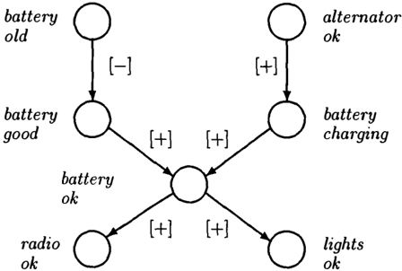
The impact of evidence on a given node can be calcu lated by taking the sign of the change in probability at the evidence node and multiplying it by the sign of every link in the sequence of links that connect it to the node of interest. To see how this works, con sider the example in Figure 1 which is an adaptation of fragment of the car diagnosis network of Henrion et al. (1994). If we observe that the radio is dead, so that the probability of the radio being ok decreases, p(radio ok) = [-], and we want to know the impact of this on the state of the battery we calculate the effect as[-]®[+]®[+]. With the definition of sign multipli cation in Table 1 this gives a change in p(battery good) of [-]. If we also observed that the lights were not ok, and wanted to assess the impact of both pieces of ev idence on the probability that the battery was good, we would establish the two individual effects and sum
them using EB ( Table 2). QCNs are very similar, the main differences being that they are abstractions of possibilistic and Dempster-Shafer belief networks as
| 可可gg3 [?] 一 [0] [?] [?] foj [?] |
| + [0] [-] [?) [-] [-] (?) [?) [?) [?) |
well as probabilistic networks, and that, in general, the qualitative influences between variables need more than one sign to define them. Formally, a QCN is a pair G = ( V, Q), where V is a set of variables or nodes in the graph, once again represented by a capital let ter, and Q is a set of sets of qualitative relations among the values of the variables. The qualitative relations are based upon the derivatives that relate the differ ent values of the variables together. In the case of a probabilistic QCN we have:
Definition 3 (qualitative derivative) The qualita tive derivative [:;f��)] relating the probability ofC tak ing value c1 to the probability of A taking value a1 has the value[+], if, for all a2 and X:
Derivatives with values (-] and [0] are defined by re placing 2: with ::; and =. The similarity of Defini tions 1 and 3 means that it is no surprise to find that the propagation of qualitative changes in the value of
variables is once again performed using® and Ef). If we write the qualitative value of the change in probability of variable A taking value a1 as [Llp(a1)] then:
and the overall effect of multiple changes is calculated using Ef). Now, a link in a QCN is normally specified by a number of qualitative values-one for each relevant derivative, which means one for every pair of values, one from each variable, of the two variables joined by the link-while, as stated above a link in a QPN is completely specified by a single value. This means that despite their similarities the two methods differ in their representation of the same information. How ever, when we have a binary probabilistic link, things are rather simpler. In this case, the condition on the derivative relating p(c) to p(a) being [+] is:
which means that if [�%t�lJ = [+] it is necessarily the case that L��c�)] = [ -] and, furthermore the rela tion between p(c) and p(-.c) makes it necessary that [d!)(:VJ = [-] and [�;(��)] = [+). These derivatives express exactly the same as a positive qualitative in fluence between binary valued A and C (if a> -.a and c >-.c)-as a becomes more probable, c becomes more probable as well. It is also the case that in this binary case [�;?�D = [�l:n so that links are symmetric. The upshot of this is that binary probabilistic QCNs are equivalent to binary QPNs, and their links can be summarised by a single qualitative value which is the qualitative derivative relating the "true" values of the links that the node connects. Thus, by investigating binary probabilistic QCNs we simultaneously develop results applicable to work involving QPNs, and this is what will be undertaken in the rest of this paper, refering to both systems simultaneously as QP/CNs.
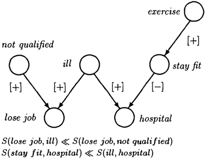
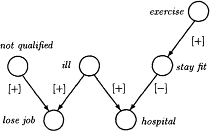
Consider the QP/CN in Figure 2 which gives some in formation about illness and employment. If I become ill it is more likely than before that I will lose my job and more likely that I will have to go to hospital. In addition, if it is discovered that I am not qualified, it becomes more likely that I will lose my job. However, regular exercise makes it more likely that I will be fit, and staying fit makes it less likely that I will end up in hospital. Consider further that it is known that I am ill. Propagating the effect of this information in our QP/CN tells us that both ending up in hospital and los ing my job become more likely since both hypotheses have value[+]. Thus it is not clear which is most likely. Distinguishing which of these competing hypotheses is more likely is the first problem that we will address
in this paper. Also consider what happens if I both become ill and exercise-the first makes hospital more likely, the second makes it less likely. Propagation of the effects of both these peices of information in the QP/CN yields a value of [?] for the change in probabil ity of the hypothesis so that we cannot say how it will change. This problem of competing influences is the second point we will address.
3 DISTINGUISHING TRUTH
The problem that we face is one of over-abstraction, and it is one well known in qualitative physics. One of the methods used to handle it is the use of landmarks (Bobrow 1984), that is distinguishing important values of variables and calculating changes relative to them. Currently QP/CNs handle links that cause a change in the descendant when the parent changes. If we dis tinguish 1 and 0, which are the obvious landmarks for probability theory, we can also distinguish increases to 1, decreases to 0, and links in which the change in the descendent is to a value of 1 or 0. More formally we denote an increase to 1 as (f], a decrease to zero as [±], and introduce a new kind of qualitative influence based on the absolute value of the conditionals:
Definition 4 (categorical influence) We say that A positively categorically influences C, written g[++] (A,C), ifffor all X, p(cla,X) = 1.
which it is easy to see will ensure that p(c I a) = 1 so that whenever p(a) increases to 1, p(c) increases to 1. We can similarly define an negative categor ical influence g[--] (A, C) which ensures that when ever p( a) increases to 1, p( c) decreases to 0 by making p(c I a, X) = 0. Clearly neither of these types of in fluence is symmetric since, for instance, the fact that p(c) is 1 whenever p(a) is 1 does not mean that p(a) is 1 whenever p(c) is 1. Thus a categorical influence be tween A and C does not imply a categorical influence between C and A. In order to propagate values with
the new influences we need to extend the definition of @ to that in Table 3.
| @ | [++] [+] (0 ] [-] [--] [?] | ||
|---|---|---|---|
| rfl | [t] | [+] [0] [-] | [?] |
| [+] | [+] [+] | [jJ (0] [-] [-] | [?] |
| [0] | [0] [0] | [OJ [o] [0] | [0] |
| [-] | [-] [-] | (0] [+] [+] | (?] |
| [±l | [-] | [-] (0] [+] [+] | [?] |
| [?] | [?] [?) | (0] [?] (?] | (?] |
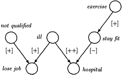
This is sufficient to solve the problem of competing hy potheses in the special case that one of the hypotheses is connected to an observed event by a chain of cat egorical influences. For example, consider Figure 3 in which the representation of my recent history is up dated to make it more realistic. Here, when it is known that I am ill, we find that !:ip(hospital) = [+], while tip (lose job) = rfJ' so that we know that it is at least as likely that I will lose my job as it is that I will have to go to hospital.
To combine categorical and qualitative influences, we need to define a new version of Ef). Initially it might seem as though we have 16 possible cases to consider every possible combination of the two types of influ ence. However, two are ruled out by the restrictive probability distribution that comes with a categorical influence:
Property 5 (restricted representation) If there is an influence s[++l (A, C) then there can be no influence S[--] (X, C) and vice-versa.
Proof: For s[++l(A,C) we require p(c I a,X) = 1 and thus p(c I a, x) = 1. For sr--l(x, C) we require p(c I x , A) = 0 and thus p(c I x ,a) = 0. These re quirements are clearly contradictory, and so the two influences may not occur together.D
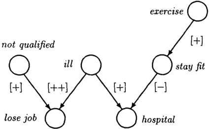
As a result there is no way that changes to 1 and 0 can conflict since the influences that cause them cannot affect the same node. This reduces the possible cases of conflict between the influences, and all the legal combinations of induced change in the probability of a node are given in Table 4. With this table we can solve the problem of conflicting influences. Consider the version of recent events according to my mother ( Figure 4) who believes that as soon as I became ill, it was inevitable that I would end up in hospital. Thus, for her, knowing that I was ill immediately outweighed all the hard work I had put in taking exercise, and /).p( hospital) = [t].
However, landmarks do not solve every problem. It is easy to imagine real situations in which conflicting evidence will cause a problem for QP /C Ns which are free of categorical influences. In qualitative reasoning circles the realised inadequacy of landmarks led to the development of 'order of magnitude' techniques, and these are what we propose to apply next.
| EB | [t] | [+] | [0] | [-] | [.). ] | [?] |
|---|---|---|---|---|---|---|
| [t] | [t] | [t] | [t] | [t] | [?] | |
| [+] | m | [+] | [+] | [?] | [ :!:] | [?] |
| [OJ | m | [+] | [0] | [-] | [±] | [?] |
| [-] | m | [?] | [-] | [-] | [ :!:] | [?] |
| [±l | [±] | [±] | [±] | [ :!:] | [?] | |
| [?] | [?] | [?] | [?] | [?] | [?] | [_? ] |
4 RELATIVE MAGNITUDES
The problem of conflicting evidence is precisely the sort of problem that order of magnitude systems such as ROM[K] (Dague 1993) were designed to overcome. ROM[K] is based on the idea that the order of magni tude of two quantities, Q1 and Q2, is usually expressed in terms of their relative sizes. Within ROM(K] there are four possible ways of expressing this relation: Q1
| (Al) | A�A | (A9) | A "" 1 -7 [ A ] = ( + ] |
| (A2) | A�B-?B�A | {AlO) | A«B ++ B�(B+A) |
| (A3) | A�B,B�C-7A�C | (All) | A«B,B""C-?A«C |
| (A4) | A""B-7B"'A | (A12) | A�B,[C] [AJ-7 (A+C)�(B+C) |
| (A5) | A,.... B,B ""C-7A"' C | (A13) | A""B, [G] [A]-7(A+C)"' (B+C) |
| (A6) | A�B-7A"'B | (A14) | A""(A+A) |
| (A7) | A�B-7C.A � C.B | (A15) | A'/:- B ++ (A-B)"'A or (B-A)"'B |
| (A8) | A "' B-7 C.A"'C.B | (P35) | A'/:- B -7 C.A '/:- C.B |
| (P3) | A«B-7C.A« C.B | {P36) | A'/:- B,C«A-7C«(A-B) |
| (P26) | A"'B-7B"'A | (P38) | A'/:- B,C�A,D�B-7C '/:-D |
is negligible wrt Q2, Q1 « Q2, Q1 is distant from Q2, Ql '/:- Q2, Q1 is comparable to Q2, Q1 "' Q2, and Ql is close to Q2, Q 1 � Q2· Once the relation between pairs of quantities is specified, it is possible to deduce new relations by applying the axioms and properties of ROM[K], some of which are reproduced in Figure 5.
Together, these relations, axioms, and properties en able us to solve our on-going problems of competing influences and hypotheses by further refining the lan guage of QP/CNs. To do this we must start deal ing with the magnitude of the probabilities and in fluences. We denote the magnitude of the change in the probability of A as j.6.p(A)I, and the magnitude of the influence between A and C as JS(A, C) I, and ex press their relative magnitudes using the relations of ROM[K], noting that again symmetry is lost so that relations change between causal and evidential direc tions. Then, provided that we have a QP/CN in which the relative magnitude of the influences is known, we can apply the rules in Figure 5 to establish the relative sizes of changes at nodes of interest. Thus:
Property 6 (relative magnitude) Given jS(A, C)j reh jS(B, D)l, and J.6.p(A)j reh J.6.p{B)j, where reh, reb E { � , .... , '/:- , «}, then j.6.p(C)I rels /.6-p(D)I is given by Table 5 and the obvious symmetrical results.
Proof: The change at C is jAp(A)j · JS(A, C) I, and likewise for that at D. Thus we need the rela tive magnitude of the products. {i) For jAp(A) I « 1.6-p(B)j and jS(A, C) I« JS(B, D) I, the result comes from P3 and Pll. (ii) For j.6.p(A)I « j.6.p(B)I and jS(A, C) I '/:- !S(B, D)\, we apply P3, P35 and P36 to get /.6-p(A)!·IS(B, D)I + IAp(B)I·!S(A, C)l « jAp(B)I· IS(B, D) I. Since we already know (from P3) that jAp(A)I·IS(A, C)!« j.6.p(A)l·lS(B, D) I, this gives us lAp(A)I . IS(A, C) I+ lAp( B) I· IS(A, C)l « 1.6-p(B)l . lS(B, D) I from which the result follows. (iii) For 1.6-p(A)I « jAp(B)I and IS( A, C)!"' IS(B, D)f, the re sult comes from A8, All and P3. (iv) For /.6-p(A)I « j.6.p(B)j and jS(A,C)j � IS(B,D)I, the result comes from A6, A7, All and P3. ( v ) For jAp(A)I '/:- j.6.p(B)I and !S(A, C) I 'f. IS(B, D) I, the result comes from the fact that 'f. is deliberately not transitive so that no relation between the products can be established. (vi) For jAp(A)I ¢ !.6-p(B)I and IS( A, C) I ,___ jS(B, D) I, we have the same explanation. (vii) For j.6.p(A)I '1: jAp(B)I and jS(A, C) I � lS(B, D) I, the result comes from A7, P35 and P38. (viii) For 1.6-p(A)I"' j.6.p(B)I and IS( A, C) I "' IS(B, D)!, the result comes from A8 and A5. (ix) For j.6.p(A)!"" !.6-p(B)I and !S(A, C) I� IS(B, D) I, the result comes from A5, A6, A7 and A8. All other results may be obtained by symmetry 0.
| reb | ||||
|---|---|---|---|---|
| � | "' | � | «: | |
| � | � | ""' | :/!. | «: |
| ""' | ""' | ""' | u | « |
| :/!. | :/!. | u | u | «: |
| «: | «: | « | « | « |
This result allows us to do two things. Firstly, it en ables us to propagate the effect of evidence in a QP/CN so that we can distinguish which of several compet ing hypotheses is most strongly supported by given evidence. Consider Figure 6 which gives another ver sion of recent events, and ponder what happens when I lose my job. The influence of losing the job on being ill is much smaller than the influence of los ing the job on not being qualified, S(lose job, ill) « S(lose job, not qualified), and since j.6.p(lose job)i � j.6.p(lose job)! we can use Property 6 with reh as« and reb as � to find that rela must be «. Thus j.6.p(ill)l « j.6.p(not qualified)!, and we know that the change in p(ill) is much less than p(not qualified).
Secondly Property 6 allows us to establish the effect of two competing pieces of information. If B influences C rather than D, then the relation given by Table 5 is that between the change in p( c) induced by the change in p( a), and that induced by the change in p(b). When
the influences compete the changes are in opposite di rections, and immediately we have:
Property 7 (comparison) If we have JS(A, C )j rel1 JS(B, D)J, and J�p(A)J reb J�p(B)J, where rel1, reb E {�, .... , �, «}, and JS(A, C)J and JS(B, D) I have oppo site signs, then [�p(C)] is given by Table 5 and the obvious symmetrical results.
Table 6: How to establish the sign of the change at C ( Property 7).
reh
| reb | ||||
|---|---|---|---|---|
| ::::: | rv | '/! | � | |
| ::::: rv 1!. � | [ ?) [ ?] [�p(B)] [�p(B)i | [ ?) [ ? ] [ ?) [�p(B)] | [�p(B ) ] [ ?] [ ? ] [�p(B)] | [�p( B) ] [�p ( B)] f � � � � j � �P B] |
To see how this property may be used, consider Fig ure 6 once again. Given that the influence of be ing ill on going to hospital is much greater than the influence of staying fit on not going to hospi tal ( J S(stay fit, hospital) I « JS(ill, hospital) I), and that there is a roughly equal increase in the proba bility of my staying fit ( due to knowledge of my ex ercising ) and being ill (J�p(stay fit)J ::::: J�p(ill)J) we can predict that there is an increase in the prob ability of my going to hospital when I become ill ([�p(hospital)] = [�p( ill)]).
Thus using ROM [ K ] allows us to solve the problem of competing influences in any situation where rela tive magnitude information is available-clearly many more situations than possess categorical links-and so improves on the results obtained by distinguishing truth. However, ROM [ K ] does not have enough nu merical information to fully distinguish between com peting hypotheses, only being able to predict which hypothesis undergoes the greatest change in probabil- ity. To tell which hypothesis becomes most likely when influences are not categorical we must turn to absolute order of magnitude methods.
5 ABSOLUTE MAGNITUDES
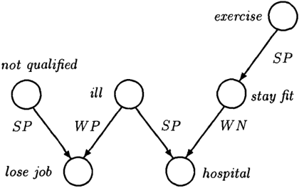
A suitable method for absolute order of magnitude rea soning, which revolves around the propagation of in terval probability values, is discussed by Dubois et al. ( 1992) in the context of quantified syllogistic reason ing. In this section we adapt it to fit QP/CNs. We start by identifying suitable interval values for both influences between nodes, changes at nodes, and the values at nodes. Here we use a very basic set for rea sons of brevity-more complex sets could be used if desired-and provide each with a label. The label of an interval is merely a means of referring to it, there is no claim that it is a natural linguistic interpretation of the interval. For the influences we have intervals cor responding to 'Strongly Positive' (SP), 'Weakly Posi tive' (W P), 'Zero' (Z), 'Weakly Negative' (W N) and ' Strongly Negative' (SN):
where the open intervals explicitly do not allow the modelling of categorical influences. Note that, once again, these influences are not symmetrical. For both changes and values we have 'Complete Positive' ( C P), 'Big Positive' (BP), ' Medium Positive' (M P), 'Little Positive' (LP) and 'Zero' (Z):
The definitions of 'Little Negative' (LN), 'Medium Negative' (M N), 'Big Negative' (BN) and 'Complete Negative' (CN) are symmetrical. When propagating absolute order of magnitude quantities, we multiply change by influence to get Table 7 The ?s in this ta-
| CP | BP | MP | LP | z | |
|---|---|---|---|---|---|
| SP | ? | ? | lMP, LP] | LP | z |
| WP | ? | ? | ? | LP | z |
| z | z | z | z | z | z |
ble arise because the results of these combinations de pend upon the comparative values of o: and ,8, and the combination of influences and changes is thus "almost robust" ( Dubois et al. 1992). If we take o: � ,8 and 1-,8 � o:, which are reasonable since typical values ( to create equally wide intervals ) would be ,8 � 0.33 and o: � 0.5, then we have Table 8. Results of combining
with negative influences and changes can be obtained by symmetry. where intervals such as [M P, LP] in-
| CP | BP | MP | LP | z | |
|---|---|---|---|---|---|
| SP | ��P, MPJ | ��P, MPJ | ��P, L�J | LP | z |
| WP | [MP,LP] | [MP,LP] | [MP,LP] | LP | z |
| z | z | z | z | z | z |
dicate that the result falls somewhere in the interval created by the outer bounds of the named intervals.
If we then provide for the comparison of intervals, for instance by 2:int (Parsons 1995b) where [a, b] 2:int [c , d] iff a 2: c and b 2: d, and negation by mapping across zero into the symmetric interval, we can re solve conflicting influences. For example, consider Fig ure 7 in which the influences have now been given ab solute orders of magnitude. Consider what happens when it is known that I both exercise and become ill. Taking into account the size of the priors, we have �p(exercise) = M P and D.p(ill) = BP. Using Ta ble 8 gives D.p(stay fit) = [M P, LP] so that we can calculate the effect of staying fit on going to hospital as �p(hospital)stay fit= [[M N, LN], LN] = [M N, LN]. The other influence on the probability of going to hospital is being ill, and clearly D.p(hospital)w = [BP, M P]. Since i[BP, M P]i 2:int j[M N, LN]j, the biggest effect on the probability of going to hospital is being ill, and �p(hospital) = [+].
To resolve competing hypotheses, we need to be able to combine changes and prior values, and with our set of intervals we get Table 9. Prior values are given across the top, changes down the side. Again the re sults are almost robust, with those given based upon the same values of o: and f3 as before. Note that only certain combinations are possible; where they are not, the' corresponding triple of prior, change, and influence cannot occur together. Now, if we are given the abso lute value of the prior probabilities of the competing
| CP | BP | MP | LP | z | |
|---|---|---|---|---|---|
| CP BP MP LP z LN MN BN CN | CP | [CP, BP] BP [BP, MP) [BP, Z] [LP, Z] | [CP,MP] [CP, MP) MP [MP, Z] [MP,Z) | [CP,BP] [CP, MP] [BP,LP) LP [LP,Z) | CP BP MP LP z |
hypotheses, we can resolve their competition. For ex ample, consider that the prior values of p(lose job) and p(hospital) are both LP, then, if �p(exercise) = M P and D.p(not qualified) = BP, then �p(hospital) = [MN,LN] and D.p(lose job) = [MP,LP]. We can use this information along with Table 9 to deter mine the posterior values p*(lose job)= [CP, LP] and p* (hospital) = [LP, Z] which by application of 2:int tells us that it is more likely that I will lose my job than go to hospital.
Thus the use of absolute orders of magnitude provides a solution to both the problem of competing hypothe ses, and that of competing influences. Note that this method may be implemented either by the use of pre compiled tables as discussed here, or more flexibly and less efficiently by the direct use of interval arithmentic.
6 SUMMARY
This paper has discussed various means of refining qualitative probabilistic reasoning to make it less sus ceptible to the problems of choosing between compet ing hypotheses, and of predicting the effect of conflict ing influences. The first method we considered was the identification of extreme probabilities, and the cate gorical influences that cause such values to arise. This solved both problems, but only in the special case in which hypotheses are affected by a categorial influ ence. To provide more general results we used relative order of magnitude reasoning to give a good solution to the problem of conflicting influences. However, the relative method did not fully solve the problem of con flicting hypotheses, and so an absolute order of magni tude scheme was introduced. This gave a satisfactory solution to both problems.
These different schemes provide a battery of methods for extending QP/CNs which can be employed when the basic QP/CN framework is not sufficiently expres sive. Clearly refining the representation will increase computational complexity, and the right degree of re finement will be determined by the particular situation
to which the methods are being applied. The greater degrees of refinement are sufficient to make QP/CNs similar in scope to the ��:-calculus (Darwiche & Gold szmidt 1994). While lack of space precludes a detailed comparison we can briefly point out three basic differ ences between the systems. Firstly, even when fully refined, QPfCNs are mainly concerned with changes in probabilities rather than probabilities themselves, unlike the ��:-calculus. Secondly, QP/CNs do not re quire the use of infinitesimals in order to be consis tent with probability theory, and so could be consid ered a more correct approach. Finally, the ��:-calculus achieves order-of-magnitude reasoning by defining an absolute scale from which different values are taken, in contrast to the purely relative method, based on ROM[K] that is introduced here. Thus, while the ��: calculus is very similar to the absolute order of mag nitude scheme introduced in Section 5, it is rather dif ferent to the other refinements discussed in this paper.
Acknowledgements
Thanks to Ann Radda for financial support when I lost my job through illness, to John Fox for making avail able facilities at the Imperial Cancer Research Fund, and to Kathy Laskey, Marek Druzdzel, and the anony mous referees for helpful comments.
References
Benferhat, S.; Dubois, D.; and Prade, H. 1993. Ar gumentative inference in uncertain and inconsistent knowledge bases. In Proceedings of the 9th Conference on Uncertainty in Artificial Intelligence.
Bobrow, D. G. 1984. Qualitative Reasoning about Physical Systems. Amsterdam: North-Holland.
Cooper, G. F. 1990. The computational complexity of probabilistic inference using belief networks. Artificial Intelligence 42:393-405.
Dague, P. 1993. Symbolic reasoning with relative or ders of magnitude. In Proceedings of the 13th Interna tional Joint Conference on Artificial Intelligence.
Darwiche, A., and Goldszmidt, M. 1994. On the rela tion between kappa calculus and probabilistic reason ing. In Proceedings of the 10th Conference on Uncer tainty in Artificial Intelligence.
Darwiche, A. 1993. Argument calculus and networks. In Proceedings of the 9th Conference on Uncertainty in Artificial Intelligence.
Druzdzel, M. J., and Henrion, M. 1993. Efficient prop agation in qualitative probabilistic networks. In Pro ceedings of the 11th National Conference on Artificial Intelligence.
Dubois, D., and Prade, H. 1988. Possibility Theory: An Approach to Computerised Processing of Uncer tainty. New York: Plenum Press.
Dubois, D.; Prade, H.; God6, 1.; and Lopez de Mantaras, R. 1992. A symbolic approach to reasoning with linguistic quantifiers. In Proceedings of the 8th Conference on Uncertainty in Artificial Intelligence.
Fox, J.; Krause, P.; and Ambler, S. 1992. Arguments, contradictions and practical reasoning. In Proceedings of the 10th European Conference on Artificial Intelli gence.
Goldszmidt, M. 1992. Qualitative probabilities: a no rmative framework for commonsense reasoning. Ph.D. Dissertation, University of California at Los Angeles.
Henrion, M., and Druzdzel, M. J. 1990. Qualitative propagation and scenario-based approaches to expla nation of probabilistic reasoning. In Proceedings of the 6th Con ference on Uncertainty in Artificial Intel ligence.
Henrion, M.; Provan, G.; Favero, B. D.; and Sanders, G. 1994. An experimental comparison of numerical and qualitative probabilistic reasoning. In Proceedings of the 10th Conference on Uncertainty in Artificial In telligence.
Michelena, N. F. 1991. Monotonic influence diagra ms: application to optimal and robust design . Ph.D. Dissertation, University of California at Berkeley.
Milgram, P. R. 1981. Good news and bad news: rep resentation theorems and applications. Bell Journal of Economics 12:380-391.
Parsons, S., and Mamdani, E. H. 1993. On reasoning in networks with qualitative uncertainty. In Proceed ings of the 9th Conference on Uncertainty in Artificial Intelligence.
Parsons, S. 1995a. Further results in qualitative un certainty. International Journal of Uncertainty, Fuzzi ness, and Knowledge Based Systems 3, (in press).
Parsons, S. 1995b. Qualitative approaches to reasoning under uncertainty. Cambridge, MA: MIT Press, (to appear).
Pearl, J. 1988. Probabilistic reasoning in intelligent systems; networks of plausible inference. San Mateo, CA: Morgan Kaufmann.
Shafer, G. 1976. A mathematical theory of evidence. Princeton, NJ: Princeton University Press.
Wellman, M. P. 1990. Formulation of tradeoffs in planning under uncertainty. London: Pitman.
Wellman, M. P. 1993. Personal communication.
Zadeh, L. A. 1978. Fuzzy sets as a basis for a theory of possibility. Fuzzy Sets and Systems 1:1-28.