Representing Conversations for Scalable Overhearing

Gery Gutnik Gal A. Kaminka

Computer Science Department Bar Ilan University Ramat Gan 52900, Israel [email protected] [email protected]

Abstract

Open distributed multi-agent systems are gaining interest in the academic community and in industry. In such open settings, agents are often coordinated using standardized agent conversation protocols. The representation of such protocols (for analysis, validation, monitoring, etc) is an important aspect of multi-agent applications. Recently, Petri nets have been shown to be an interesting approach to such representation, and radically different approaches using Petri nets have been proposed. However, their relative strengths and weaknesses have not been examined. Moreover, their scalability and suitability for different tasks have not been addressed. This paper addresses both these challenges. First, we analyze existing Petri net representations in terms of their scalability and appropriateness for overhearing, an important task in monitoring open multi-agent systems. Then, building on the insights gained, we introduce a novel representation using Colored Petri nets that explicitly represent legal joint conversation states and messages. This representation approach offers significant improvements in scalability and is particularly suitable for overhearing. Furthermore, we show that this new representation offers a comprehensive coverage of all conversation features of FIPA conversation standards. We also present a procedure for transforming AUML conversation protocol diagrams (a standard humanreadable representation), to our Colored Petri net representation.

1. Introduction

Open distributed multi-agent systems (MAS) are composed of multiple, independently-built agents that carry out mutually-dependent tasks. In order to allow inter-operability of agents of different designs and implementation, the agents often coordinate using standardized interaction protocols, or conversations. Indeed, the multi-agent community has been investing a significant effort in developing standardized Agent Communication Languages (ACL) to facilitate sophisticated multi-agent systems (Finin, Labrou, & Mayfield, 1997; Kone, Shimazu, & Nakajima, 2000; ChaibDraa, 2002; FIPA site, 2003). Such standards define communicative acts, and on top of them, interaction protocols , ranging from simple queries as to the state of another agent, to complex negotiations by auctions or bidding on contracts. For instance, the FIPA Contract Net Interaction Protocol (FIPA Specifications, 2003b) defines a concrete set of message sequences that allows the interacting agents to use the contract net protocol for negotiations.

Various formalisms have been proposed to describe such standards (e.g., Smith & Cohen, 1996; Parunak, 1996; Odell, Parunak, & Bauer, 2000, 2001b; AUML site, 2003). In particular, AUMLAgent Unified Modelling Language -is currently used in the FIPA-ACL standards

Gutnik & Kaminka

(FIPA Specifications, 2003a, 2003b, 2003c, 2003d; Odell, Parunak, & Bauer, 2001a) 1 . UML 2.0 (AUML site, 2003), a new emerging standard influenced by AUML, has the potential to become the FIPA-ACL standard (and a forthcoming IEEE standard) in the future. However, for the moment, a large set of FIPA specifications remains formalized using AUML. While AUML is intended for human readability and visualization, interaction protocols should ideally be represented in a way that is amenable to automated analysis, validation and verification, online monitoring, etc.

Lately, there is increasing interest in using Petri nets (Petri Nets site, 2003) in modelling multi-agent interaction protocols (Cost, 1999; Cost, Chen, Finin, Labrou, & Peng, 1999, 2000; Lin, Norrie, Shen, & Kremer, 2000; Nowostawski, Purvis, & Cranefield, 2001; Purvis, Hwang, Purvis, Cranefield, & Schievink, 2002; Cranefield, Purvis, Nowostawski, & Hwang, 2002; Ramos, Frausto, & Camargo, 2002; Mazouzi, Fallah-Seghrouchni, & Haddad, 2002; Poutakidis, Padgham, & Winikoff, 2002). There is broad literature on using Petri nets to analyze the various aspects of distributed systems (e.g. in deadlock detection as shown by Khomenco & Koutny, 2000), and there has been recent work on specific uses of Petri nets in multi-agent systems, e.g., in validation and testing (Desel, Oberweis, & Zimmer, 1997), in automated debugging and monitoring (Poutakidis et al., 2002), in dynamic interpretation of interaction protocols (Cranefield et al., 2002; de Silva, Winikoff, & Liu, 2003), in modelling agents behavior induced by their participation in a conversation (Ling & Loke, 2003) and in interaction protocols refinement allowing modular construction of complex conversations (Hameurlain, 2003).

However, key questions remain open on the use of Petri nets for conversation representation. First, while radically different approaches to representation using Petri nets have been proposed, their relative strengths and weaknesses have not been investigated. Second, many investigations have only addressed restricted subsets of the features needed in representing complex conversations such as those standardized by FIPA (see detailed discussion of previous work in Section 2). Finally, no procedures have been proposed for translating human-readable AUML protocol descriptions into the corresponding machine-readable Petri nets.

This paper addresses these open challenges in the context of scalable overhearing . Here, an overhearing agent passively tracks many concurrent conversations involving multiple participants, based solely on their exchanged messages, while not being a participant in any of the overheard conversations itself (Novick & Ward, 1993; Busetta, Serafini, Singh, & Zini, 2001; Kaminka, Pynadath, & Tambe, 2002; Poutakidis et al., 2002; Busetta, Dona, & Nori, 2002; Legras, 2002; Gutnik & Kaminka, 2004a; Rossi & Busetta, 2004). Overhearing is useful in visualization and progress monitoring (Kaminka et al., 2002), in detecting failures in interactions (Poutakidis et al., 2002), in maintaining organizational and situational awareness (Novick & Ward, 1993; Legras, 2002; Rossi & Busetta, 2004) and in non-obtrusively identifying opportunities for offering assistance (Busetta et al., 2001, 2002). For instance, an overhearing agent may monitor the conversation of a contractor agent engaged in multiple contract-net protocols with different bidders and bid callers, in order to detect failures.

We begin with an analysis of Petri net representations, with respect to scalability and overhearing. We classify representation choices along two dimensions affecting scalability:

1. (FIPA Specifications, 2003c) is currently deprecated. However, we use this specification since it describes many important features needed in modelling multi-agent interactions.

(i) the technique used to represent multiple concurrent conversations; and (ii) the choice of representing either individual or joint interaction states. We show that while the runtime complexity of monitoring conversations using different approaches is the same, choices along these two dimensions have significantly different space requirements, and thus some choices are more scalable (in the number of conversations) than others. We also argue that representations suitable for overhearing require the use of explicit message places, though only a subset of previously-explored techniques utilized those.

Building on the insights gained, the paper presents a novel representation that uses Colored Petri nets (CP-nets) in which places explicitly denote messages, and valid joint conversation states. This representation is particularly suited for overhearing as the number of conversations is scaled-up. We show how this representation can be used to represent essentially all features of FIPA AUML conversation standards, including simple and complex interaction building blocks, communicative act attributes such as message guards and cardinalities, nesting, and temporal aspects such as deadlines and duration.

To realize the advantages of machine-readable representations, such as for debugging (Poutakidis et al., 2002), existing human-readable protocol descriptions must be converted to their corresponding Petri net representations. As a final contribution in this paper, we provide a skeleton semi-automated procedure for converting FIPA conversation protocols in AUML to Petri nets, and demonstrate its use on a complex FIPA protocol. While this procedure is not fully automated, it takes a first step towards addressing this open challenge.

This paper is organized as follows. Section 2 presents the motivation for our work. Sections 3 through 6 then present the proposed representation addressing all FIPA conversation features including basic interaction building blocks (Section 3), message attributes (Section 4), nested & interleaved interactions (Section 5), and temporal aspects (Section 6). Section 7 ties these features together: It presents a skeleton algorithm for transforming an AUML protocol diagram to its Petri net representation, and demonstrates its use on a challenging FIPA conversation protocol. Section 8 concludes. The paper rounds up with three appendixes. The first provides a quick review of Petri nets. Then, to complete coverage of FIPA interactions, Appendix B provides additional interaction building blocks. Appendix C presents a Petri net of a complex conversation protocol, which integrates many of the features of the developed representation technique.

2. Representations for Scalable Overhearing

Overhearing involves monitoring conversations as they progress, by tracking messages that are exchanged between participants (Gutnik & Kaminka, 2004a). We are interested in representations that can facilitate scalable overhearing, tracking many concurrent conversations, between many agents. We focus on open settings, where the complex internal state and control logic of agents is not known in advance, and therefore exclude discussions of Petri net representations which explicitly model agent internals (e.g., Moldt & Wienberg, 1997; Xu & Shatz, 2001). Instead, we treat agents as black boxes, and consider representations that commit only to the agent's conversation state (i.e., its role and progress in the conversation).

The suitability of a representation for scalable overhearing is affected by several facets. First, since overhearing is based on tracking messages, the representation must be able to explicitly represent the passing of a message (communicative act) from one agent to another

Gutnik & Kaminka

(Section 2.1). Second, the representation must facilitate tracking of multiple concurrent conversations. While the tracking runtime is bounded from below by the number of messages (since in any case, all messages are overheard and processed), space requirements may differ significantly (see Sections 2.2-2.3).

2.1 Message-monitoring versus state-monitoring

We distinguish two settings for tracking the progress of conversations, depending on the information available to the tracking agent. In the first type of setting, which we refer to as state monitoring , the tracking agent has access to the internal state of the conversation in one or more of the participants, but not necessarily to the messages being exchanged. The other settings involves message monitoring , where the tracking agent has access only to the messages being exchanged (which are externally observable ), but cannot directly observe the internal state of the conversation in each participant. Overhearing is a form of message monitoring.

Representations that support state monitoring use places to denote the conversation states of the participants. Tokens placed in these places (the net marking) denote the current state. The sending or receiving of a message by a participant is not explicitly represented, and is instead implied by moving tokens (through transition firings) to the new state places. Thus, such a representation essentially assumes that the internal conversation state of participants is directly observable by the monitoring agent. Previous work utilizing state monitoring includes work by Cost (1999), Cost et al. (1999, 2000), Lin et al. (2000), Mazouzi et al. (2002), Ramos et al. (2002).

The representation we present in this paper is intended for overhearing tasks, and cannot assume that the conversation states of overheard agents are observable. Instead, it must support message monitoring, where in addition to using tokens in state places (to denote current conversation state), the representation uses message places , where tokens are placed when a corresponding message is overheard. A conversation-state place and a message place are connected via a transition to a state place denoting the new conversation state. Tokens placed in these originating places-indicating a message was received at an appropriate conversation state-will cause the transition to fire, and for the tokens to be placed in the new conversation state place. Thus the new conversation state is inferred from "observing" a message. Previous investigations, that have used explicit message places, include work by Cost (1999), Cost et al. (1999, 2000), Nowostawski et al. (2001), Purvis et al. (2002), Cranefield et al. (2002), Poutakidis et al. (2002) 2 . These are discussed in depth below.

2.2 Representing a Single Conversation

Two representation variants are popular within those that utilize conversation places (in addition to message places): Individual state representations use separate places and tokens for the state of each participant (each role). Thus, the overall state of the conversation is represented by different tokens marking multiple places. Joint state representations use a single place for each joint conversation state of all participants. The placement of a token

2. Cost (1999), Cost et al. (1999, 2000) present examples of both state- and message- monitoring representations.

within such a place represents the overhearing agent's belief that the participants are in the appropriate joint state.

Most previous representations use individual states. In these, different markings distinguish a conversation state where one agent has sent a message, from a state where the other agent received it. The net for each conversation role is essentially built separately, and is merged with the other nets, or connected to them via fusion places or similar means.

Cost (1999), Cost et al. (1999, 2000) have used CP-nets with individual state places for representing KQML and FIPA interaction protocols. Transitions represent message events, and CP-net features, such as token colors and arc expressions, are used to represent AUML message attributes and sequence expressions. The authors also point out that deadlines (a temporal aspect of interaction) can be modelled, but no implementation details are provided. Cost (1999) also proposed using hierarchical CP-nets to represent hierarchical multi-agent conversations.

Purvis et al. (2002), Cranefield et al. (2002) represented conversation roles as separate CP-nets, where places denote both interaction messages and states, while transitions represent operations performed on the corresponding communicative acts such as send, receive, and process. Special in/out places are used to pass net tokens between the different CP-nets, through special get/put transitions, simulating the actual transmission of the corresponding communicative acts.

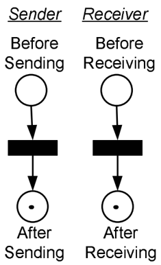
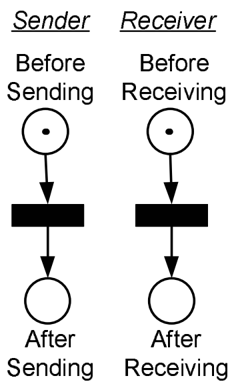
In principle, individual-state representations require two places in each role, for every message. For a given message, there would be two individual places for the sender (before sending and after sending), and similarly two more for each receiver (before receiving and after receiving). All possible conversation states-valid or not-can be represented. For a single message and two roles, there are two places for each role (four places total), and four possible conversation states: message sent and received, sent and not received, not sent but incorrectly believed to have been received, not sent and not received. These states can be represented by different markings. For instance, a conversation state where the message has been sent but not received is denoted by a token in the 'after-sending' place of the sender and another token in the 'before-receiving' place of the receiver . This is summarized in the following proposition:

Proposition 1 Given a conversation with R roles and a total of M possible messages, an individual state representation has space complexity of O ( MR ) .

While the representations above all represent each role's conversation state separately, many applications of overhearing only require representation of valid conversation states (message not sent and not received, or sent and received). Indeed, specifications for interaction protocols often assume the use of underlying synchronization protocols to guarantee delivery of messages (Paurobally & Cunningham, 2003; Paurobally, Cunningham, & Jennings, 2003). Under such an assumption, for every message, there are only two joint states regardless of the number of roles. For example, for a single message and three roles-a sender and two receivers, there are two places and two possible markings: A token in a before sending/receiving place represents a conversation state where the message has not yet been sent by the sender (and the two receivers are waiting for it), while a token in a after sending/receiving place denotes that the message has been sent and received by both receivers .

Gutnik & Kaminka

Nowostawski et al. (2001) utilize CP-nets where places denote joint conversation states. They also utilize places representing communicative acts. Poutakidis et al. (2002) proposed a representation based on Place-Transition nets (PT-nets)-a more restricted representation of Petri nets that has no color. They presented several interaction building blocks, which could then fit together to model additional conversation protocols. In general, the following proposition holds with respect to such representations:

Proposition 2 Given a conversation with R roles and a total of M possible messages, a joint state representation that represents only legal states has space complexity of O ( M ) .

The condition of representing only valid states is critical to the complexity analysis. If all joint conversation states-valid and invalid-are to be represented, the space complexity would be O ( M R ) . In such a case, an individual-state representation would have an advantage. This would be the case, for instance, if we do not assume the use of synchronization protocols, e.g., where the overhearing agent may wish to track the exact system state even while a message is underway (i.e., sent and not yet received).

2.3 Representing Multiple Concurrent Conversations

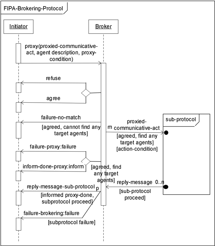
Propositions 1 and 2 above address the space complexity of representing a single conversation. However, in large scale systems an overhearing agent may be required to monitor multiple conversations in parallel. For instance, an overhearing agent may be monitoring a middle agent that is carrying multiple parallel instances of a single interaction protocol with multiple partners, e.g., brokering (FIPA Specifications, 2003a).

Some previous investigations propose to duplicate the appropriate Petri net representation for each monitored conversation (Nowostawski et al., 2001; Poutakidis et al., 2002). In this approach, every conversation is tracked by a separate Petri-net, and thus the number of Petri nets (and their associated tokens) grows with the number of conversations (Proposition 3). For instance, Nowostawski et al. (2001) shows an example where a contract-net protocol is carried out with three different contractors, using three duplicate CP-nets. This is captured in the following proposition:

Proposition 3 A representation that creates multiple instances of a conversation Petri net to represent C conversations, requires O ( C ) net structures, and O ( C ) bits for all tokens.

Other investigations take a different approach, in which a single CP-net structure is used to monitor all conversations of the same protocol. The tokens associated with conversations are differentiated by their token color (Cost, 1999; Cost et al., 1999, 2000; Lin et al., 2000; Mazouzi et al., 2002; Cranefield et al., 2002; Purvis et al., 2002; Ramos et al., 2002). For example, by assigning each token a color of the tuple type 〈 sender, receiver 〉 , an agent can differentiate multiple tokens in the same place and thus track conversations of different pairs of agents 3 . Color tokens use multiple bits per token; up to log C bits are required to differentiate C conversations. Therefore, the number of bits required to track C conversations using C tokens is C log C . This leads to the following proposition.

3. See Section 4 to distinguish between different conversations by the same agents.

Proposition 4 A representation that uses color tokens to represent C multiple instances of a conversation, requires O (1) net structures, and O ( C log C ) bits for all tokens.

Due to the constants involved, the space requirements of Proposition 3 are in practice much more expensive than those of Proposition 4. Proposition 3 refers to the creation of O ( C ) Petri networks, each with duplicated place and transition data structures. In contrast, Proposition 4 refers to bits required for representing C color tokens on a single CP net. Moreover, in most practical settings, a sufficiently large constant bound on the number of conversations may be found, which will essentially reduce the O (log C ) factor to O (1) .

Based on Propositions 1-4, it is possible to make concrete predictions as to the scalability of different approaches with respect to the number of conversations, roles. Table 1 shows the space complexity of different approaches when modelling C conversations of the same protocol, each with a maximum of R roles, and M messages, under the assumption of underlying synchronization protocols. The table also cites relevant previous work.

Table 1: Scalability of different representations

	Representing Multiple Conversations (of Same Protocol)
	Multiple CP- or PT-nets (Proposition 3)	Using color tokens, single CP-net (Proposition 4)
Individual States (Proposition 1)	Space: O ( MRC )	Space: O ( MR + C log C ) Cost (1999), Cost et al. (1999, 2000), Lin et al. (2000), Cranefield et al. (2002), Purvis et al. (2002), Ramos et al. (2002), Mazouzi et al. (2002)
Joint States (Proposition 2)	Space: O ( MC ) Nowostawski et al. (2001), Poutakidis et al. (2002)	Space: O ( M + C log C ) This paper

Building on the insights gained from Table 1, we propose a representation using CP-nets where places explicitly represent joint conversation states (corresponding to the lower-right cell in Table 1), and tokens color is used to distinguish concurrent conversations (as in the upper-right cell in Table 1). As such, it is related to the works that have these features, but as the table demonstrates, is a novel synthesis.

Our representation uses similar structures to those found in the works of Nowostawski et al. (2001) and Poutakidis et al. (2002). However, in contrast to these previous investigations, we rely on token color in CP-nets to model concurrent conversations, with space complexity O ( M + C log C ) . We also show (Sections 3-6) how it can be used to cover a variety of conversation features not covered by these investigations. These features include representation of a full set of FIPA interaction building blocks, communicative act attributes (such as message guards, sequence expressions, etc.), compact modelling of concurrent conversations, nested and interleaved interactions, and temporal aspects.

3. Representing Simple & Complex Interaction Building Blocks

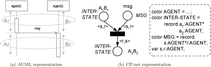
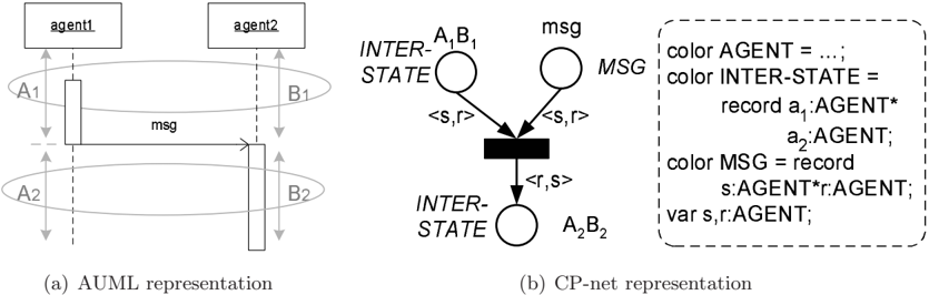
This section introduces the fundamentals of our representation, and demonstrates how various simple and complex AUML interaction messages, used in FIPA conversation standards (FIPA Specifications, 2003c), can be implemented using the proposed CP-net representation. We begin with a simple conversation, shown in Figure 1-a using an AUML protocol diagram. Here, agent 1 sends an asynchronous message msg to agent 2 .

✁✂✄☎✆✝

/a0 ✞✟✠✡☛

✛✜✢

Figure 1: Asynchronous message interaction.

To represent agent conversation protocols, we define two types of places, corresponding to messages and conversation states. The first type of net places, called message places , is used to describe conversation communicative acts. Tokens placed in message places indicate that the associated communicative act has been overheard. The second type of net places, agent places , is associated with the valid joint conversation states of the interacting agents. Tokens placed in agent places indicate the current joint state of the conversation within the interaction protocol.

Transitions represent the transmission and receipt of communicative acts between agents. Assuming underlying synchronization protocols, a transition always originates within a jointstate place and a message place, and targets a joint conversation state (more than one is possible-see below). Normally, the current conversation state is known (marked with a token), and must wait the overhearing of the matching message (denoted with a token at the connected message place). When this token is marked, the transition fires, automatically marking the new conversation state.

Figure 1-b presents CP net representation of the earlier example of Figure 1-a. The CPnet in Figure 1-b has three places and one transition connecting them. The A 1 B 1 and the A 2 B 2 places are agent places, while the msg place is a message place. The A and B capital letters are used to denote the agent 1 and the agent 2 individual interaction states respectively (we have indicated the individual and the joint interaction states over the AUML diagram in Figure 1-a, but omit these annotations in later figures). Thus, the A 1 B 1 place indicates a joint interaction state where agent 1 is ready to send the msg communicative act to agent 2 ( A 1 ) and agent 2 is waiting to receive the corresponding message ( B 1 ). The msg message place corresponds to the msg communicative act sent between the two agents. Thus, the transmission of the msg communicative act causes the agents to transition to the A 2 B 2

place. This place corresponds to the joint interaction state in which agent 1 has already sent the msg communicative act to agent 2 ( A 2 ) and agent 2 has received it ( B 2 ).

The CP-net implementation in Figure 1-b also introduces the use of token colors to represent additional information about interaction states and communicative acts. The token color sets are defined in the net declaration, i.e. the dashed box in Figure 1-b. The syntax follows the standard CPN ML notation (Wikstrom, 1987; Milner, Harper, & Tofte, 1990; Jensen, 1997a). The AGENT color identifies the agents participating in the interaction, and is used to construct the two compound color sets.

The INTER-STATE color set is associated with agent places, and represents agents in the appropriate joint interaction states. It is a record 〈 a 1 , a 2 〉 , where a 1 and a 2 are AGENT color elements distinguishing the interacting agents. We apply the INTER-STATE color set to model multiple concurrent conversations using the same CP-net. The second color set is MSG , describing interaction communicative acts and associated with message places. The MSG color token is a record 〈 a s , a r 〉 , where a s and a r correspond to the sender and the receiver agents of the associated communicative act. In both cases, additional elements, such as conversation identification, may be used. See Section 4 for additional details.

In Figure 1-b, the A 1 B 1 and the A 2 B 2 places are associated with the INTER-STATE color set, while the msg place is associated with the MSG color set. The place color set is written in italic capital letters next to the corresponding place. Furthermore, we use the s and r AGENT color type variables to denote the net arc expressions. Thus, given that the output arc expression of both the A 1 B 1 and the msg places is 〈 s, r 〉 , the s and r elements of the agent place token must correspond to the s and r elements of the message place token. Consequently, the net transition occurs if and only if the agents of the message correspond to the interacting agents. The A 2 B 2 place input arc expression is 〈 r, s 〉 following the underlying intuition that agent 2 is going to send the next interaction communicative act.

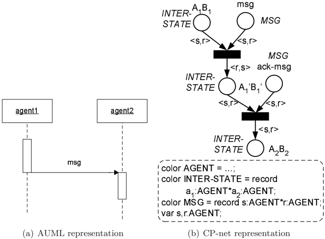
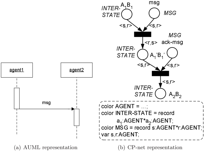
Figure 2-a shows an AUML representation of another interaction building block, synchronous message passing, denoted by the filled solid arrowhead. Here, the msg communicative act is sent synchronously from agent 1 to agent 2 , meaning that an acknowledgement on msg communicative act must always be received by agent 1 before the interaction may proceed.

The corresponding CP-net representation is shown in Figure 2-b. The interaction starts in the A 1 B 1 place and terminates in the A 2 B 2 place. The A 1 B 1 place represents a joint interaction state where agent 1 is ready to send the msg communicative act to agent 2 ( A 1 ) and agent 2 is waiting to receive the corresponding message ( B 1 ). The A 2 B 2 place denotes a joint interaction state, in which agent 1 has already sent the msg communicative act to agent 2 ( A 2 ) and agent 2 has received it ( B 2 ). However, since the CP-net diagram represents synchronous message passing, the msg communicative act transmission cannot cause the agents to transition directly from the A 1 B 1 place to the A 2 B 2 place. We therefore define an intermediate A ′ 1 B ′ 1 agent place. This place represents a joint interaction state where agent 2 has received the msg communicative act and is ready to send an acknowledgement on it ( B 1 '), while agent 1 is waiting for that acknowledgement ( A ′ 1 ). Taken together, the msg communicative act causes the agents to transition from the A 1 B 1 place to the A ′ 1 B ′ 1 place, while the acknowledgement on the msg message causes the agents to transition from the A ′ 1 B ′ 1 place to the A 2 B 2 place.

➶➹➘➴➷➬

➺ ➻

➼ ➽

➾➚➪

Figure 2: Synchronous message interaction.

Transitions in a typical multi-agent interaction protocols are composed of interaction building blocks, two of which have been presented above. Additional interaction buildingblocks, which are fairly straightforward (or have appeared in previous work, e.g., Poutakidis et al., 2002) are presented in Appendix B. In the remainder of this section, we present two complex interactions building blocks that are generally common in multi-agent interactions: XOR-decision and OR-parallel.

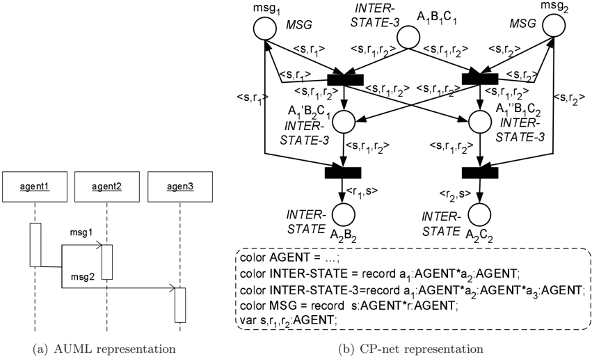
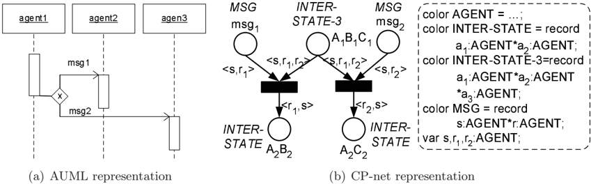
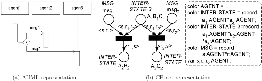
We begin with the XOR-decision interaction. The AUML representation to this building block is shown in Figure 3-a. The sender agent agent 1 can either send message msg 1 to agent 2 or message msg 2 to agent 3 , but it can not send both msg 1 and msg 2 . The non-filled diamond with an 'x' inside is the AUML notation for this constraint.

❶❷❸❹❺❻

❼❽❾❿➀➁

➂➃➄➅➆

➌➍➎➏➐➑

➒➓➔→➣↔↕

➙➛➜

❒❮❰

/a234/a235/a236

/a253/a254/a255✌✝ ✟✎✏✑✒ ✓ ✔✕

Figure 3: XOR-decision messages interaction.

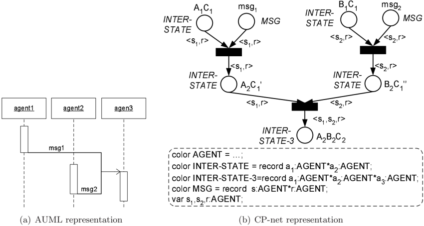
Figure 3-b shows the corresponding CP-net. Again, the A , B and C capital letters are used to denote the interaction states of agent 1 , agent 2 and agent 3 , respectively. The

interaction starts from the A 1 B 1 C 1 place and terminates either in the A 2 B 2 place or in the A 2 C 2 place. The A 1 B 1 C 1 place represents a joint interaction state where agent 1 is ready to send either the msg 1 communicative act to agent 2 or the msg 2 communicative act to agent 3 ( A 1 ); and agent 2 and agent 3 are waiting to receive the corresponding msg 1 / msg 2 message ( B 1 / C 1 ). To represent the A 1 B 1 C 1 place color set, we extend the INTER-STATE color set to denote a joint interaction state of three interacting agents, i.e. using the INTERSTATE-3 color set. The msg 1 communicative act causes the agents to transition to A 2 B 2 place. The A 2 B 2 place represents a joint interaction state where agent 1 has sent the msg 1 message ( A 2 ), and agent 2 has received it ( B 2 ). Similarly, the msg 2 communicative act causes agents agent 1 and agent 3 to transition to A 2 C 2 place. Exclusiveness is achieved since the single agent token in A 1 B 1 C 1 place can be used either for activating the A 1 B 1 C 1 → A 2 B 2 transition or for activating the A 1 B 1 C 1 → A 2 C 2 transition, but not both.

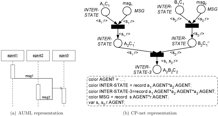
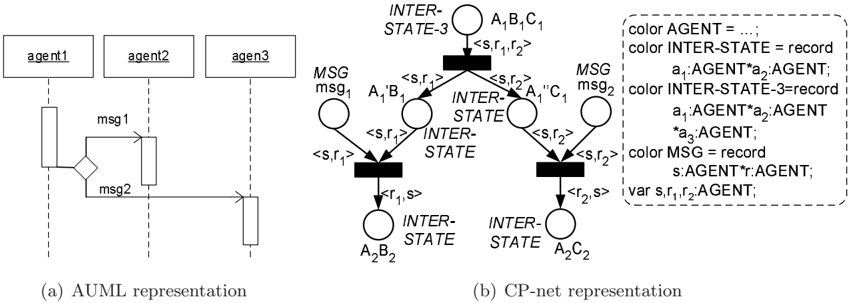
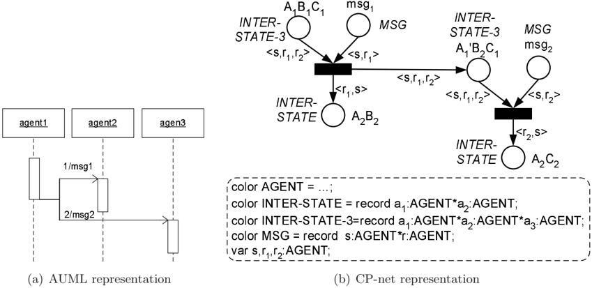
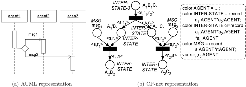
A similar complex interaction is the OR-parallel messages interaction. Its AUML representation is presented in Figure 4-a. The sender agent, agent 1 , can send message msg 1 to agent 2 or message msg 2 to agent 3 , or both. The non-filled diamond is the AUML notation for this constraint.

/a252/a253/a254/a255✞✠☛

/a246/a247/a248/a249/a250/a251

✟ ✁ /a0

✂ ✡ ✄

Figure 4: OR-parallel messages interaction.

Figure 4-b shows the CP-net representation of the OR-parallel interaction. The interaction starts from the A 1 B 1 C 1 place but it can be terminated in the A 2 B 2 place, or in the A 2 C 2 place, or in both. To represent this inclusiveness of the interaction protocol, we define two intermediate places, the A ′ 1 B 1 place and the A ′′ 1 C 1 place. The A ′ 1 B 1 place represents a joint interaction state where agent 1 is ready to send the msg 1 communicative act to agent 2 ( A ′ 1 ) and agent 2 is waiting to receive the message ( B 1 ). The A ′′ 1 C 1 place has similar meaning, but with respect to agent 3 . As normally done in Petri nets, the transition connecting the A 1 B 1 C 1 place to the intermediate places duplicates any single token in A 1 B 1 C 1 place into two tokens going into the A ′ 1 B 1 and the A ′′ 1 C 1 places. Consequently, the two parts of the OR-parallel interaction can be independently executed.

4. Representing Interaction Attributes

We now extend our representation to allow additional interaction aspects, useful in describing multi-agent conversation protocols. First, we show how to represent interaction

■❏❑▲▼ ◆❖/a80◗❘ ❙ ❚❯

message attributes, such as guards, sequence expressions, cardinalities and content (FIPA Specifications, 2003c). We then explore in depth the representation of multiple concurrent conversations (on the same CP net).

Figure 5-a shows a simple agent interaction using an AUML protocol diagram. This interaction is similar to the one presented in Figure 1-a in the previous section. However, Figure 5-a uses an AUML message guard-condition-marked as [ condition ] -that has the following semantics: the communicative act is sent from agent 1 to agent 2 if and only if the condition is true.

❄❅❆❇❈ ❉❊❋●❍ ■ ❏❑

Figure 5: Message guard-condition

The guard-condition implementation in our Petri net representation uses transition guards (Figure 5-b), a native feature for CP nets. The AUML guard condition is mapped directly to the CP-net transition guard. The CP-net transition guard is indicated on the net inscription next to the corresponding transition using square brackets. The transition guard guarantees that the transition is enabled if and only if the transition guard is true.

In Figure 5-b, we also extend the color of tokens to include information about the communicative act being used and its content. We extend the MSG color set definition to a record 〈 s, r, t, c 〉 , where the s and r elements has the same interpretation as in previous section (sender and receiver), and the t and c elements define the message type and content, respectively. The t element is of a new color TY PE , which determines communicative act types. The c element is of a new color CONTENT , which represents communicative act content and argument list (e.g. reply-to, reply-by and etc).

The addition of new elements also allows for additional potential uses. For instance, to facilitate representation of multiple concurrent conversations between the same agents ( s and r ), it is possible to add a conversation identification field to both the MSG and INTER-STATE colors. For simplicity, we refrain from doing so in the examples in this paper.

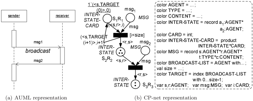
Two additional AUML communicative act attributes that can be modelled in the CP representation are message sequence-expression and message cardinality. The sequenceexpressions denote a constraint on the message sent from sender agent. There are a number of sequence-expressions defined by FIPA conversation standards (FIPA Specifications, 2003c): m denotes that the message is sent exactly m times; n..m denotes that the message is sent anywhere from n up to m times; ∗ denotes that the message is sent an arbitrary number of

times. An additional important sequence expression is broadcast , i.e. message is sent to all other agents.

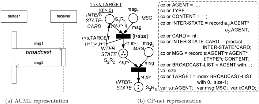
We now explain the representation of sequence-expressions in CP-nets, using broadcast as an example (Figure 6-b). Other sequence expressions are easily derived from this example. We define an INTER-STATE-CARD color set. This color set is a tuple ( 〈 a 1 , a 2 〉 , i ) consisting of two elements. The first tuple element is an INTER-STATE color element, which denotes the interacting agents as previously defined. The second tuple element is an integer that counts the number of messages already sent by an agent, i.e. the message cardinality. This element is initially assigned to 0. The INTER-STATE-CARD color set is applied to the S 1 R 1 place, where the S and R capital letters are used to denote the sender and the receiver individual interaction states respectively and the S 1 R 1 indicates the initial joint interaction state of the interacting agents. The two additional colors, used in Figure 6-b, are the BROADCAST-LIST and the TARGET colors. The BROADCAST-LIST color defines the sender broadcast list of the designated receivers, assuming that the sender must have such a list to carry out its role. The TARGET color defines indexes into this broadcast list.

❛❜❝❞❡❢❣❤✐❥❦❧

✆✝✞ ✟

➅➆➇➈➉ ➊➋➌➍➎ ➏ ➐➑

Figure 6: Broadcast sequence expression.

According to the broadcast sequence-expression semantics, the sender agent sends the same msg 1 communicative act to all the receivers on the broadcast list . The CP-net introduced in Figure 6-b models this behavior. 4 The interaction starts from the S 1 R 1 place, representing the joint interaction state where sender is ready to send the msg 1 communicative act to receiver ( S 1 ) and receiver is waiting to receive the corresponding msg 1 message ( R 1 ). The S 1 R 1 place initial marking is a single token, set by the initialization expression (underlined, next to the corresponding place). The initialization expression 1'( 〈 s, T ARGET (0) 〉 , 0) -given in standard CPN ML notation-determines that the S 1 R 1 place's initial marking is a multi-set containing a single token ( 〈 s, T ARGET (0) 〉 , 0) . Thus, the first designated receiver is assigned to be the agent with index 0 on the broadcast list, and the message cardinality counter is initiated to 0 .

4. We implement broadcast as an iterative procedure sending the corresponding communicative act separately to all designated recipients.

Gutnik & Kaminka

The msg 1 message place initially contains multiple tokens. Each of these tokens represents the msg 1 communicative act addressed to a different designated receiver on the broadcast list . In Figure 6-b, the initialization expression, corresponding to the msg 1 message place, has been omitted. The S 1 R 1 place token and the appropriate msg 1 place token together enable the corresponding transition. Consequently, the transition may fire and thus the msg 1 communicative act transmission is simulated.

The msg 1 communicative act is sent incrementally to every designated receiver on the broadcast list . The incoming arc expression ( 〈 s, r 〉 , i ) is incremented by the transition to the outgoing ( 〈 s, T ARGET ( i +1) 〉 , i + 1) arc expression, causing the receiver agent with index i +1 on the broadcast list to be selected. The transition guard constraint i < size , i.e. i < | broadcast list | , ensures that the msg 1 message is sent no more than | broadcast list | times. The msg 1 communicative act causes the agents to transition to the S 2 R 2 place. This place represents a joint interaction state in which sender has already sent the msg 1 communicative act to receiver and is now waiting to receive the msg 2 message ( S 2 ) and receiver has received the msg 1 message and is ready to send the msg 2 communicative act to sender ( R 2 ). Finally, the msg 2 message causes the agents to transition to the S 3 R 3 place. The S 3 R 3 place denotes a joint interaction state where sender has received the msg 2 communicative act from receiver and terminated ( S 3 ), while receiver has already sent the msg 2 message to sender and terminated as well ( R 3 ).

We use Figure 6-b to demonstrate the use of token color to represent multiple concurrent conversations using the same CP-net. For instance, let us assume that the sender agent is called agent 1 and its broadcast list contains the following agents: agent 2 , agent 3 , agent 4 , agent 5 and agent 6 . We will also assume that the agent 1 has already sent the msg 1 communicative act to all agents on the broadcast list . However, it has only received the msg 2 reply message from agent 3 and agent 6 . Thus, the CP-net current marking for the complete interaction protocol is described as follows: the S 2 R 2 place is marked by 〈 agent 2 , agent 1 〉 , 〈 agent 4 , agent 1 〉 , 〈 agent 5 , agent 1 〉 , while the S 3 R 3 place contains the tokens 〈 agent 1 , agent 3 〉 and 〈 agent 1 , agent 6 〉 .

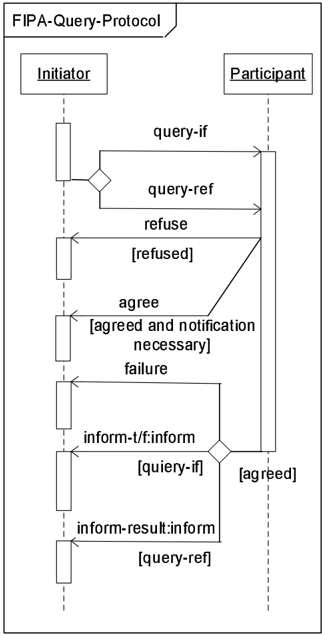
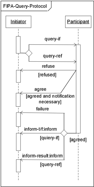
An Example . We now construct a CP-net representation of the FIPA Query Interaction Protocol (FIPA Specifications, 2003d), shown in AUML form in Figure 7, to demonstrate how the building blocks presented in Sections 3 and 4 can be put together. In this interaction protocol, the Initiator requests the Participant to perform an inform action using one of two query communicative acts, query-if or query-ref . The Participant processes the query and makes a decision whether to accept or refuse the query request. The Initiator may request the Participant to respond with either an accept or refuse message, and for simplicity, we will assume that this is always the case. In case the query request has been accepted, the Participant informs the Initiator on the query results. If the Participant fails, then it communicates a failure . In a successful response, the Participant replies with one of two versions of inform ( inform-t/f or inform-result ) depending on the type of initial query request.

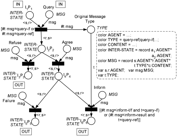
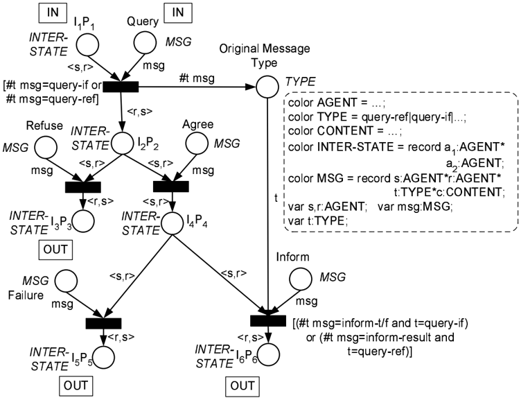
The CP-net representation of the FIPA Query Interaction Protocol is presented in Figure 8. The interaction starts in the I 1 P 1 place (we use the I and the P capital letters to denote the Initiator and the Participant roles). The I 1 P 1 place represents a joint interaction state where (i) the Initiator agent is ready to send either the query-if communicative act, or the query-ref message, to Participant ( I 1 ); and (ii) Participant is wait-

❥❦❧♠♥♦♣/a113/a114/a115/a116✉✈✇①②③④⑤

ing to receive the corresponding message ( P 1 ). The Initiator can send either a query-if or a query-ref communicative act. We assume that these acts belong to the same class, the query communicative act class. Thus, we implement both messages using a single Query message place, and check the message type using the following transition guard: [# t msg = query-if or # t msg = query-ref ] . The query communicative act causes the interacting agents to transition to the I 2 P 2 place. This place represents a joint interaction state in which Initiator has sent the query communicative act and is waiting to receive a response message ( I 2 ), and Participant has received the query communicative act and deciding whether to send an agree or a refuse response message to Initiator ( P 2 ). The refuse communicative act causes the agents to transition to I 3 P 3 place, while the agree message causes the agents to transition to I 4 P 4 place.

The Participant decision on whether to send an agree or a refuse communicative act is represented using the XOR-decision building block introduced earlier (Figure 3-b). The I 3 P 3 place represents a joint interaction state where Initiator has received a refuse communicative act and terminated ( I 3 ) and Participant has sent a refuse message and terminated as well ( P 3 ). The I 4 P 4 place represents a joint interaction state in which Initiator has received an agree communicative act and is now waiting for further response from

/a210/a211

⑥

⑩❶❷❸❹

/a212/a213

Figure 8: FIPA Query Interaction Protocol - CP-net representation.

Participant ( I 4 ) and Participant has sent an agree message and is now deciding which response to send to Initiator ( P 4 ). At this point, the Participant agent may send one of the following communicative acts: inform-t/f , inform-result and failure . The choice is represented using another XOR-decision building block, where the inform-t/f and informresult communicative acts are represented using a single Inform message place. The failure communicative act causes a transition to the I 5 P 5 place, while the inform message causes a transition to the I 6 P 6 place. The I 5 P 5 place represents a joint interaction state where Participant has sent a failure message and terminated ( P 5 ), while Initiator has received a failure and terminated ( I 5 ). The I 6 P 6 place represents a joint interaction state in which Participant has sent an inform message and terminated ( P 6 ), while Initiator has received an inform and terminated ( I 6 ).

The implementation of the [ query-if ] and the [ query-ref ] message guard conditions requires a detailed discussion. These are not implemented in a usual manner in view of the fact that they depend on the original request communicative act. Thus, we create a special intermediate place that contains the original message type marked " Original Message Type " in the figure. In case an inform communicative act is sent, the transition guard verifies that the inform message is appropriate to the original query type. Thus, an inform-t/f communicative act can be sent only if the original query type has been query-if and an inform-result message can be sent only if the original query type has been query-ref .

5. Representing Nested & Interleaved Interactions

In this section, we extend the CP-net representation of previous sections to model nested and interleaved interaction protocols. We focus here on nested interaction protocols. Nevertheless, the discussion can also be addressed to interleaved interaction protocols in a similar fashion.

FIPA conversation standards (FIPA Specifications, 2003c) emphasize the importance of nested and interleaved protocols in modelling complex interactions. First, this allows reuse of interaction protocols in different nested interactions. Second, nesting increases the readability of interaction protocols.

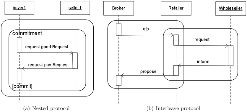
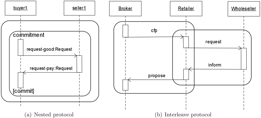
The AUML notation annotates nested and interleaved protocols as round corner rectangles (Odell et al., 2001a; FIPA Specifications, 2003c). Figure 9-a shows an example of a nested protocol 5 , while Figure 9-b illustrates an interleaved protocol. Nested protocols have one or more compartments. The first compartment is the name compartment. The name compartment holds the (optional) name of the nested protocol. The nested protocol name is written in the upper left-hand corner of the rectangle, i.e. commitment in Figure 9a. The second compartment, the guard compartment, holds the (optional) nested protocol guard. The guard compartment is written in the lower left-hand corner of the rectangle, e.g. [ commit ] in Figure 9-a. Nested protocols without guards are equivalent to nested protocols with the [ true ] guard.

➁➂➃➄➅➆

➇➈➉➊➋➌➍

/a211/a212/a213/a214/a215/a216

/a217/a218/a219/a220 /a221/a222 /a223 /a224

/a235 /a236/a237 /a238/a239 /a240/a241/a242/a243/a244 /a245

Figure 9: AUML nested and interleaved protocols examples.

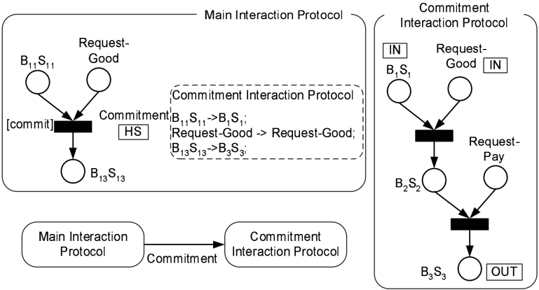
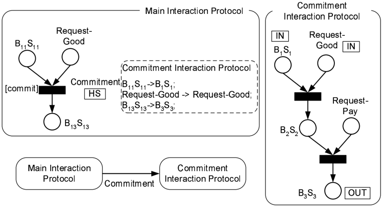
Figure 10 describes the implementation of the nested interaction protocol presented in Figure 9-a by extending the CP-net representation to using hierarchies, relying on standard CP-net methods (see Appendix A). The hierarchical CP-net representation contains three elements: a superpage , a subpage and a page hierarchy graph. The CP-net superpage represents the main interaction protocol containing a nested interaction, while the CP-net subpage models the corresponding nested interaction protocol, i.e. the Commitment Inter-

5. Figure 9-a appears in FIPA conversation standards (FIPA Specifications, 2003c). Nonetheless, note that the request-good and the request-pay communicative acts are not part of the FIPA-ACL standards.

action Protocol . The page hierarchy graph describes how the superpage is decomposed into subpages.

➠➡➢➤ ➥➦➧➨➩➫➭➯➲➳➵ ➸➺➻➼➽➾➚➪

➶➹➘➴➷➬➮➱✃❐

Figure 10: Nested protocol implementation using hierarchical CP-nets.

Let us consider in detail the process of modelling the nested interaction protocol in Figure 9-a using a hierarchical CP-net, resulting in the net described in Figure 10. First, we identify the starting and ending points of the nested interaction protocol. The starting point of the nested interaction protocol is where Buyer 1 sends a Request-Good communicative act to Seller 1 . The ending point is where Buyer 1 receives a Request-Pay communicative act from Seller 1 . We model these nested protocol end-points as CP-net socket nodes on the superpage, i.e. Main Interaction Protocol : B 11 S 11 and Request-Good are input socket nodes and B 13 S 13 is an output socket node.

The nested interaction protocol, the Commitment Interaction Protocol , is represented using a separate CP-net, following the principles outlined in Sections 3 and 4. This net is a subpage of the main interaction protocol superpage. The nested interaction protocol starting and ending points on the subpage correspond to the net port nodes . The B 1 S 1 and Request-Good places are the subpage input port nodes, while the B 3 S 3 place is an output port node. These nodes are tagged with the IN/OUT port type tags correspondingly.

Then, a substitution transition , which is denoted using HS (Hierarchy and Substitution), connects the corresponding socket places on the superpage. The substitution transition conceals the nested interaction protocol implementation from the net superpage, i.e. the Main Interaction Protocol . The nested protocol name and guard compartments are mapped directly to the substitution transition name and guard respectively. Consequently, in Figure 10 we define the substitution transition name as Commitment and the substitution guard is determined to be [ commit ] .

The superpage and subpage interface is provided using the hierarchy inscription. The hierarchy inscription is indicated using the dashed box next to the substitution transition. The first line in the hierarchy inscription determines the subpage identity, i.e. the

Commitment Interaction Protocol in our example. Moreover, it indicates that the substitution transition replaces the corresponding subpage detailed implementation on the superpage. The remaining hierarchy inscription lines introduce the superpage and subpage port assignment. The port assignment relates a socket node on the superpage with a port node on the subpage. The substitution transition input socket nodes are related to the IN-tagged port nodes. Analogously, the substitution transition output socket nodes correspond to the OUT-tagged port nodes. Therefore, the port assignment in Figure 10 assigns the net socket and port nodes in the following fashion: B 11 S 11 to B 1 S 1 , Request-Good to Request-Good and B 13 S 13 to B 3 S 3 .

Finally, the page hierarchy graph describes the decomposition hierarchy (nesting) of the different protocols (pages). The CP-net pages, the Main Interaction Protocol and the Commitment Interaction Protocol , correspond to the page hierarchy graph nodes (Figure 10). The arc inscription indicates the substitution transition, i.e. Commitment .

6. Representing Temporal Aspects of Interactions

Two temporal interaction aspects are specified by FIPA (FIPA Specifications, 2003c). In this section, we show how timed CP-nets (see also Appendix A) can be applied for modelling agent interactions that involve temporal aspects, such as interaction duration, deadlines for message exchange, etc.

A first aspect, duration , is the interaction activity time period. Two periods can be distinguished: transmission time and response time . The transmission time indicates the time interval during which a communicative act, is sent by one agent and received by the designated receiver agent. The response time period denotes the time interval in which the corresponding receiver agent is performing some task as a response to the incoming communicative act.

The second temporal aspect is deadlines . Deadlines denote the time limit by which a communicative act must be sent. Otherwise, the corresponding communicative act is considered to be invalid. These issues have not been addressed in previous investigations related to agent interactions modelling using Petri nets. 6

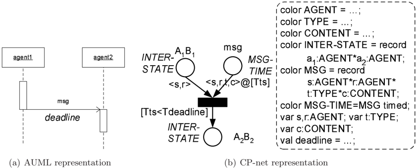
We propose to utilize timed CP-nets techniques to represent these temporal aspects of agent interactions. In doing so, we assume a global clock. 7 We begin with deadlines. Figure 11-a introduces the AUML representation of message deadlines. The deadline keyword is a variation of the communicative act sequence expressions described in Section 4. It sets a time constraint on the start of the transmission of the associated communicative act. In Figure 11-a, agent 1 must send the msg communicative act to agent 2 before the defined deadline . Once the deadline expires, the msg communicative act is considered to be invalid.

Figure 11-b shows a timed CP-net implementation of the deadline sequence expression. The timed CP-net in Figure 11-b defines an additional MSG-TIME color set associated with the net message places. The MSG-TIME color set extends the MSG color set, described in Section 4, by adding a time stamp attribute to the message token. Thus, the communicative

6. Cost et al. (1999, 2000) mention deadlines without presenting any implementation details.

7. Implementing it, we can use the private clock of an overhearing agent as the global clock for our Petri net representation. Thus, the time stamp of the message is the overhearer's time when the corresponding message was overheard.

⑨⑩❶❷❸ ❹❺❻❼❽ ❾ ❿➀

act token is a record 〈 s, r, t, c 〉 @[ Tts ] . The @[ .. ] expression denotes the corresponding token time stamp, whereas the token time value is indicated starting with a capital 'T'. Accordingly, the described message token has a ts time stamp. The communicative act time limit is defined using the val deadline parameter. Therefore, the deadline sequence expression semantics is simulated using the following transition guard: [ Tts < Tdeadline ] . This transition guard, comparing the msg time stamp against the deadline parameter, guarantees that an expired msg communicative act can not be received.

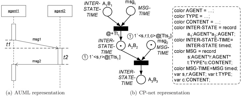
We now turn to representing interaction duration. The AUML representation is shown in Figure 12-a. The AUML time intensive message notation is used to denote the communicative act transmission time. As a rule communicative act arrows are illustrated horizontally. This indicates that the message transmission time can be neglected. However, in case the message transmission time is significant, the communicative act is drawn slanted downwards. The vertical distance, between the arrowhead and the arrow tail, denotes the message transmission time. Thus, the communicative act msg 1 , sent from agent 1 to agent 2 , has a t 1 transmission time.

③④⑤⑥

❜ ❝ ❞ ❡

❢❣❤ ✐

❥❦❧♠♥♦

Figure 12: Interaction duration.

The response time in Figure 12-a is indicated through the interaction thread length. The incoming msg 1 communicative act causes agent 2 to perform some task before sending a response msg 2 message. The corresponding interaction thread duration is denoted through the t 2 time period. Thus, this time period specifies the agent 2 response time to the incoming msg 1 communicative act.

The CP-net implementation to the interaction duration time periods is shown in Figure 12-b. The communicative act transmission time is illustrated using the timed CP-nets @+ operator. The net transitions simulate the communicative act transmission between agents. Therefore, representing a transmission time of t 1 , the CP-net transition adds a t 1 time period to the incoming message token time stamp. Accordingly, the transition @+ Tt 1 output arc expression denotes a t 1 delay to the time stamp of the outgoing token. Thus, the corresponding transition takes t 1 time units and consequently so does the msg 1 communicative act transmission time.

In contrast to communicative act transmission time, the agent interaction response time is represented implicitly. Previously, we have defined a MSG-TIME color set that indicates message token time stamps. Analogously, in Figure 12-b we introduce an additional INTERSTATE-TIME color set. This color set is associated with the net agent places and it presents the possibility to attach time stamps to agent tokens as well. Now, let us assume that A 2 B 2 and msg 2 places contain a single token each. The circled '1' next to the corresponding place, together with the multi-set inscription, indicates the place current marking. Thus, the agent and the message place tokens have a ts 1 and a ts 2 time stamps respectively. The ts 1 time stamp denotes the time by which agent 2 has received the msg 1 communicative act sent by agent 1 . The ts 2 time stamp indicates the time by which agent 2 is ready to send msg 2 response message to agent 1 . Thus, the agent 2 response time t 2 (Figure 12-a) is ts 2 -ts 1 .

7. Algorithm and a Concluding Example

Our final contribution in this paper is a skeleton procedure for transforming an AUML conversation protocol diagram of two interacting agents to its CP-net representation. The procedure is semi-automated-it relies on the human to fill in some details-but also has automated aspects. We apply this procedure on a complex multi-agent conversation protocol that involves many of the interaction building blocks already discussed.

The procedure is shown in Algorithm 1. The algorithm input is an AUML protocol diagram and the algorithm creates, as an output, a corresponding CP-net representation. The CP-net is constructed in iterations using a queue. The algorithm essentially creates the conversation net by exploring the interaction protocol breadth-first while avoiding cycles.

Lines 1-2 create and initiate the algorithm queue, and the output CP-net, respectively. The queue, denoted by S , holds the initiating agent places of the current iteration. These places correspond to interaction states that initiate further conversation between the interacting agents. In lines 4-5, an initial agent place A 1 B 1 is created and inserted into the queue. The A 1 B 1 place represents a joint initial interaction state for the two agents. Lines 7-23 contain the main loop.

We enter the main loop in line 8 and set the curr variable to the first initiating agent place in S queue. Lines 10-13 create the CP-net components corresponding to the current iteration as follows. First, in line 10, message places, associated with curr agent place, are

Algorithm 1 Create Conversation Net( input : AUML , output : CPN ) 1: S ← new queue 2: CPN ← new CP -net 3: 4: A 1 B 1 ← new agent place with color information 5: S.enqueue ( A 1 B 1 ) 6: 7: while S not empty do 8: curr ← S.dequeue () 9: 10: MP ← CreateMessagePlaces ( AUML,curr ) 11: RP ← CreateResultingAgentPlaces ( AUML,curr,MP ) 12: ( TR,AR ) ← CreateTransitionsAndArcs ( AUML,curr,MP,RP ) 13: FixColor ( AUML,CPN,MP,RP,TR,AR ) 14: 15: for each place p in RP do 16: if p was not created in current iteration then 17: continue 18: if p is not terminating place then 19: S.enqueue ( p ) 20: 21: CPN.places = CPN.places ⋃ MP ⋃ RP 22: CP.transitions = CPN.transitions ⋃ TR 23: CPN.arcs = CPN.arcs ⋃ AR 24: 25: return CPN

created using the CreateMessagePlaces procedure (which we do not detail here). This procedure extracts the communicative acts that are associated with a given interaction state, from the AUML diagram. These places correspond to communicative acts, which take agents from the joint interaction state curr to its successor(s). Then in line 11, the CreateResultingAgentPlaces procedure creates agent places that correspond to interaction state changes as a result of the communicative acts associated with curr agent place (again based on the AUML diagram). Then, in CreateTransitionsAndArcs procedure (line 12), these places are connected using the principles described in Sections 3-6. Thus, the CP-net structure (net places, transitions and arcs) is created. Finally, in line 13, the FixColor procedure adds token color elements to the CP-net structure, to support deadlines, cardinality, and other communicative act attributes.

Lines 15-19 determine which resulting agent places are inserted into the S queue for further iteration. Only non-terminating agent places, i.e. places that do not correspond to interaction states that terminate the interaction, are inserted into the queue in lines 18-19. However, there is one exception (lines 16-17): a resulting agent place, which has already been handled by the algorithm, is not inserted back into the S queue since inserting it can cause an infinite loop. Thereafter, completing the current iteration, the output CP-net, denoted

by CPN variable, is updated according to the current iteration CP-net components in lines 21-23. This main loop iterates as long as the S queue is not empty. The resulting CP-net is returned-line 25.

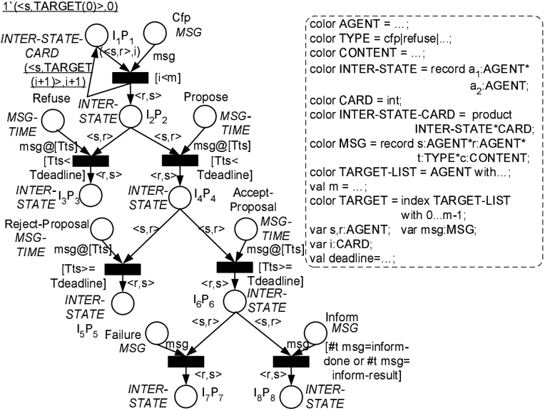
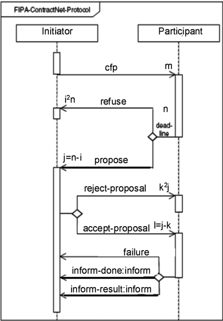
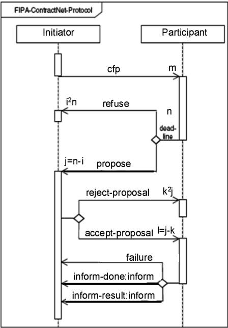
To demonstrate this algorithm, we will now use it on the FIPA Contract Net Interaction Protocol (FIPA Specifications, 2003b) (Figure 13). This protocol allows interacting agents to negotiate. The Initiator agent issues m calls for proposals using a cfp communicative act. Each of the mParticipants may refuse or counter-propose by a given deadline sending either a refuse or a propose message respectively. A refuse message terminates the interaction. In contrast, a propose message continues the corresponding interaction.

Once the deadline expires, the Initiator does not accept any further Participant response messages. It evaluates the received Participant proposals and selects one, several, or no agents to perform the requested task. Accepted proposal result in the sending of accept-proposal messages, while the remaining proposals are rejected using reject-proposal message. Reject-proposal terminates the interaction with the corresponding Participant . On the other hand, the accept-proposal message commits a Participant to perform the requested task. On successful completion, Participant informs Initiator sending either an inform-done or an inform-result communicative act. However, in case a Participant has failed to accomplish the task, it communicates a failure message.

Gutnik & Kaminka

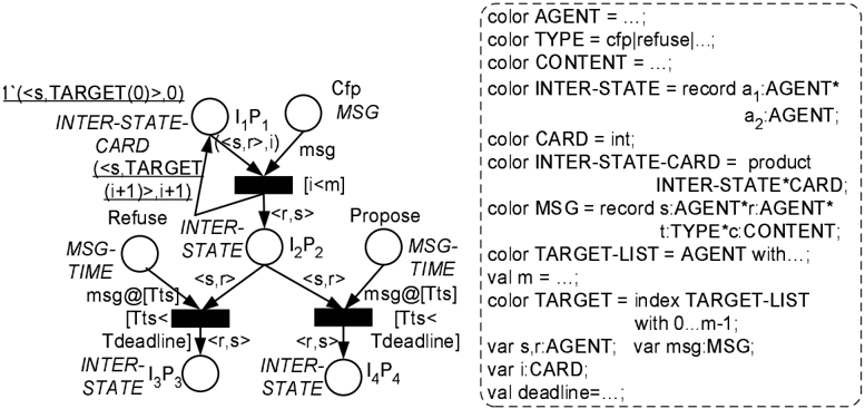
We now use the algorithm introduced above to create a CP-net, which represents the FIPA Contract Net Interaction Protocol . The corresponding CP-net model is constructed in four iterations of the algorithm. Figure 14 shows the CP-net representation after the second iteration of the algorithm, while Figure 15 shows the CP-net representation after the fourth and final iteration.

The Contract Net Interaction Protocol starts from I 1 P 1 place, which represents a joint interaction state where Initiator is ready to send a cfp communicative act ( I 1 ) and Participant is waiting for the corresponding cfp message ( P 1 ). The I 1 P 1 place is created and inserted into the queue before the iterations through the main loop begin.

First iteration . The curr variable is set to the I 1 P 1 place. The algorithm creates net places, which are associated with the I 1 P 1 place, i.e. a Cfp message place, and an I 2 P 2 resulting agent place. The I 2 P 2 place denotes an interaction state in which Initiator has already sent a cfp communicative act to Participant and is now waiting for its response ( I 2 ) and Participant has received the cfp message and is now deciding on an appropriate response ( P 2 ). These are created using the CreateMessagePlaces and the CreateResultingAgentPlaces procedures, respectively.

Then, the CreateTransitionsAndArcs procedure in line 12, connects the three places using a simple asynchronous message building block as shown in Figure 1-b (Section 3). In line 13, as the color sets of the places are determined, the algorithm also handles the cardinality of the cfp communicative act, by putting an appropriate sequence expression on the transition, using the principles presented in Figure 6-b (Section 4). Accordingly, the color set, associated with I 1 P 1 place, is changed to the INTER-STATE-CARD color set. Since the I 2 P 2 place is not a terminating place, it is inserted into the S queue.

Second iteration . curr is set to the I 2 P 2 place. The Participant agent can send, as a response, either a refuse or a propose communicative act. Refuse and Propose message places are created by CreateMessagePlaces (line 10), and resulting places I 3 P 3 and I 4 P 4 , corresponding to the results of the refuse and propose communicative acts, respectively, are created by CreateResultingAgentPlaces (line 11). The I 3 P 3 place represents a joint interaction state where Participant has sent the refuse message and terminated ( P 3 ), while Initiator has received it, and terminated ( I 3 ). The I 4 P 4 place represents the joint state in which Participant has sent the propose message ( P 4 ), while Initiator has received the message and is considering its response ( I 4 ).

In line 12, the I 2 P 2 , Refuse , I 3 P 3 , Propose and I 4 P 4 places are connected using the XOR-decision building block presented in Figure 3-b (Section 3). Then, the FixColor procedure (line 13), adds the appropriate token color attributes, to allow a deadline sequence expression (on both the refuse and the propose messages) to be implemented as shown in Figure 11-b (Section 6). The I 3 P 3 place denotes a terminating state, whereas the I 4 P 4 place continues the interaction. Thus, in lines 18-19, only the I 4 P 4 place is inserted into the queue, for the next iteration of the algorithm. The state of the net at the end of the second iteration of the algorithm is presented in Figure 14.

Third iteration . curr is set to I 4 P 4 . Here, the Initiator response to a Participant proposal can either be an accept-proposal or a reject-proposal . CreateMessagePlaces procedure in line 10 thus creates the corresponding Accept-Proposal and Reject-Proposal message places. The accept-proposal and reject-proposal messages cause the interacting agents to transition to I 5 P 5 and I 6 P 6 places, respectively. These agent places are created using the

✬✭✮✯✰ ✱✲✳✴✵ ✶ ✷✸

CreateResultingAgentPlaces procedure (line 11). The I 5 P 5 place denotes an interaction state in which Initiator has sent a reject-proposal message and terminated the interaction ( I 5 ), while the Participant has received the message and terminated as well ( P 5 ). In contrast, the I 6 P 6 place represents an interaction state where Initiator has sent an acceptproposal message and is waiting for a response ( I 6 ), while Participant has received the accept-proposal communicative act and is now performing the requested task before sending a response ( P 6 ). The Initiator agent sends exclusively either an accept-proposal or a rejectproposal message. Thus, the I 4 P 4 , Reject-Proposal , I 5 P 5 , Accept-Proposal and I 6 P 6 places are connected using a XOR-decision block (in the CreateTransitionsAndArcs procedure, line 12).

The FixColor procedure in line 13 operates now as follows: According to the interaction protocol semantics, the Initiator agent evaluates all the received Participant proposals once the deadline passes. Only thereafter, the appropriate reject-proposal and accept-proposal communicative acts are sent. Thus, FixColor assigns a MSG-TIME color set to the RejectProposal and the Accept-Proposal message places, and creates a [ Tts > = Tdeadline ] transition guard on the associated transitions. This transition guard guarantees that Initiator cannot send any response until the deadline expires, and all valid Participant responses have been received. The resulting I 5 P 5 agent place denotes a terminating interaction state, whereas the I 6 P 6 agent place continues the interaction. Thus, only I 6 P 6 agent place is inserted into the S queue.

Fourth iteration . curr is set to I 6 P 6 . This place is associated with three communicative acts: inform-done , inform-result and failure . The inform-done and the informresult messages are instances of the inform communicative act class. Thus, CreateMessagePlaces (line 10) creates only two message places, Inform and Failure . In line 11, CreateResultingAgentPlaces creates the I 7 P 7 and I 8 P 8 agent places. The failure communicative act causes interacting agents to transition to I 7 P 7 agent place, while both inform messages cause the agents to transition to I 8 P 8 agent place. The I 7 P 7 place represents a joint interaction state where Participant has sent the failure message and terminated ( P 7 ),

while Initiator has received a failure communicative act and terminated ( I 7 ). On the other hand, the I 8 P 8 place denotes an interaction state in which Participant has sent the inform message (either inform-done or inform-result ) and terminated ( P 8 ), while Initiator has received an inform communicative act and terminated ( I 8 ). The inform and failure communicative acts are sent exclusively. Thus CreateTransitionsAndArcs (line 12) connects the I 6 P 6 , Failure , I 7 P 7 , Inform and I 8 P 8 places using a XOR-decision building block. Then, FixColor assigns a [# t msg = inform-done or # t msg = inform-result ] transition guard on the transition associated with Inform message place. Since both the I 7 P 7 and the I 8 P 8 agent places represent terminating interaction states, they are not inserted into the queue, which remains empty at the end of the current iteration. This signifies the end of the conversion. The complete conversation CP-net resulting after this iteration of the algorithm is shown in Figure 15.

➪➶➹➘➴➷➬➮➱✃❐❒❮❰/a207/a208/a209/a210/a211

♣/a113/a114

Figure 15: FIPA Contract Net Interaction Protocol using CP-net after the 4 th (and final) iteration.

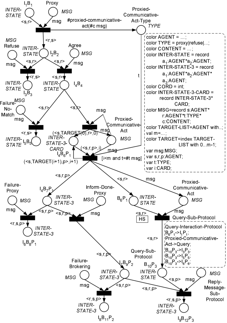
The procedure we outline can guide the conversion of many 2-agent conversation protocols in AUML to their CP-net equivalents. However, it is not sufficiently developed to address the general n-agent case. Appendix C presents a complex example of a 3-agent conversation protocol, which was successfully converted manually, without the guidance of the algorithm. This example incorporates many advanced features of our CP-net representation technique and would have been beyond the scope of many previous investigations.

8. Summary and Conclusions

Over recent years, open distributed MAS applications have gained broad acceptance both in the multi-agent academic community and in real-world industry. As a result, increasing attention has been directed to multi-agent conversation representation techniques. In particular, Petri nets have recently been shown to provide a viable representation approach (Cost et al., 1999, 2000; Nowostawski et al., 2001; Mazouzi et al., 2002).

However, radically different approaches have been proposed to using Petri nets for modelling multi-agent conversations. Yet, the relative strengths and weaknesses of the proposed techniques have not been examined. Our work introduces a novel classification of previous investigations and then compares these investigations addressing their scalability and appropriateness for overhearing tasks.

Based on the insights gained from the analysis, we have developed a novel representation, that uses CP-nets in which places explicitly represent joint interaction states and messages. This representation technique offers significant improvements (compared to previous approaches) in terms of scalability, and is particularly suitable for monitoring via overhearing. We systematically show how this representation covers essentially all the features required to model complex multi-agent conversations, as defined by the FIPA conversation standards (FIPA Specifications, 2003c). These include simple & complex interaction building blocks (Section 3 & Appendix B), communicative act attributes and multiple concurrent conversations using the same CP-net (Section 4), nested & interleaved interactions using hierarchical CP-nets (Section 5) and temporal interaction attributes using timed CP-nets (Section 6). The developed techniques have been demonstrated, throughout the paper, on complex interaction protocols defined in the FIPA conversation standards (see in particular the example presented in Appendix C). Previous approaches could handle some of these examples (though with reduced scalability), but only a few were shown to cover all the required features.

Finally, the paper presented a skeleton procedure for semi-automatically converting an AUML protocol diagrams (the chosen FIPA representation standard) to an equivalent CPnet representation. We have demonstrated its use on a challenging FIPA conversation protocol, which was difficult to represent using previous approaches.

We believe that this work can assist and motivate continuing research on multi-agent conversations including such issues as performance analysis, validation and verification (Desel et al., 1997), agent conversation visualization, automated monitoring (Kaminka et al., 2002; Busetta et al., 2001, 2002), deadlock detection (Khomenco & Koutny, 2000), debugging (Poutakidis et al., 2002) and dynamic interpretation of interaction protocols (Cranefield et al., 2002; de Silva et al., 2003). Naturally, some issues remain open for future work. For example, the presented procedure addresses only AUML protocol diagrams representing two agent roles. We plan to investigate an n-agent version in the future.

Acknowledgments

The authors would like to thank the anonymous JAIR reviewers for many useful and informative comments. Minor subsets of this work were also published as LNAI book chapter (Gutnik & Kaminka, 2004b). K. Ushi deserves many thanks.

Appendix A. A Brief Introduction to Petri Nets

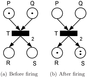
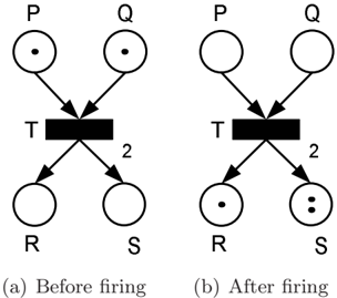
Petri nets (Petri Nets site, 2003) are a widespread, established methodology for representing and reasoning about distributed systems, combining a graphical representation with a comprehensive mathematical theory. One version of Petri nets is called Place/Transition nets (PT-nets) (Reisig, 1985). A PT-net is a bipartite directed graph where each node is either a place or a transition (Figure 16). The net places and transitions are indicated through circles and rectangles respectively. The PT-net arcs support only place → transition and transition → place connections, but never connections between two places or between two transitions. The arc direction determines the input/output characteristics of the place and the transition connected. Thus, given an arc, P → T , connecting place P and transition T , we will say that place P is an input place of transition T and vice versa transition T is an output transition of place P . The P → T arc is considered to be an output arc of place P and an input arc of transition T .

➐

➑

➣

↔

Figure 16: A PT-net example.

A PT-net place may be marked by small black dots called tokens . The arc expression is an integer, which determines the number of tokens associated with the corresponding arc. By convention, an arc expression equal to 1 is omitted. A specific transition is enabled if and only if its input places marking satisfies the appropriate arc expressions. For example, consider arc P → T to be the only arc to connect place P and transition T . Thus, given that this arc has an arc expression 2, we will say that transition T is enabled if and only if place P is marked with two tokens. In case the transition is enabled, it may fire/occur . The transition occurrence removes tokens from the transition input places and puts tokens to the transition output places as specified by the arc expressions of the corresponding input/output arcs. Thus, in Figures 16-a and 16-b, we demonstrate PT-net marking before and after transition firing respectively.

Although computationally equivalent, a different version of Petri nets, called Colored Petri nets (CP-nets) (Jensen, 1997a, 1997b, 1997c), offers greater flexibility in compactly representing complex systems. Similarly to the PT-net model, CP-nets consist of net places, net transitions and arcs connecting them. However, in CP-nets, tokens are not just single bits, but can be complex, structured, information carriers. The type of additional information carried by the token, is called token color , and it may be simple (e.g., an integer or a string), or complex (e.g. a record or a tuple). Each place is declared by a place color set to

only match tokens of particular colors. A CP-net place marking is a token multi-set (i.e., a set in which a member may appear more than once) corresponding to the appropriate place color set. CP-net arcs pass token multi-sets between the places and transitions. CP-net arc expressions can evaluate token multi-sets and may involve complex calculation procedures over token variables declared to be associated with the corresponding arcs.

The CP-net model introduces additional extensions to PT-nets. Transition guards are boolean expressions, which constrain transition firings. A transition guard associated with a transition tests tokens that pass through a transition, and will only enable the transition firings if the guard is successfully matched (i.e., the test evaluates to true). The CP-net transition guards, together with places color sets and arc expressions, appear as a part of net inscriptions in the CP-net.

In order to visualize and manage the complexity of large CP-nets, hierarchical CP-nets (Huber, Jensen, & Shapiro, 1991; Jensen, 1997a) allow hierarchical representations of CPnets, in which sub-CP nets can be re-used in higher-level CP nets, or abstracted away from them. Hierarchical CP-nets are built from pages, which are themselves CP-nets. Superpages present a higher level of hierarchy, and are CP-nets that refer to subpages , in addition to transitions and places. A subpage may also function as a superpage to other subpages. This way, multiple hierarchy levels can be used in a hierarchical CP-net structure.

The relationship between a superpage and a subpage is defined by a substitution transition , which substitutes a corresponding subpage instance on the CP-net superpage structure as a transition in the superpage. The substitution transition hierarchy inscription supplies the exact mapping of the superpage places connected to the substitution transition (called socket nodes ), to the subpage places (called port nodes ). The port types determine the characteristics of the socket node to port node mappings. A complete CP-net hierarchical structure is presented using a page hierarchy graph , a directed graph where vertices correspond to pages, and directed edges correspond to direct superpage-subpage relationships.

Timed CP-nets (Jensen, 1997b) extend CP-nets to support the representation of temporal aspects using a global clock . Timed CP-net tokens have an additional color attribute called time stamp , which refers to the earliest time at which the token may be used. Time stamps can be used by arc expression and transition guards, to enable a timed-transition if and only if it satisfies two conditions: (i) the transition is color enabled , i.e. it satisfies the constraints defined by arc expression and transition guards; and (ii) the tokens are ready , i.e. the time of the global clock is equal to or greater than the tokens' time stamps. Only then can the transition fire.

Appendix B. Additional Examples of Conversation Representation Building Blocks

This appendix presents some additional interaction building blocks to those already described in Section 3. The first is the AND-parallel messages interaction (AUML representation shown in Figure 17-a). Here, the sender agent 1 sends both the msg 1 message to agent 2 and the msg 2 message to agent 3 . However, the order of the two communicative acts is unconstrained.

The representation of AND-parallel in our CP-net representation is shown in Figure 17-b. The A 1 B 1 C 1 , A 2 B 2 , A 2 C 2 , msg 1 and msg 2 places are defined similarly to Figures 3-b and

➪➶➹ ➘

➴➷➬➮➱✃

✔ ✕

✖ ✗ ✘ ✙

Figure 17: AND-parallel messages interaction.

4-b in Section 3. However, we also define two additional intermediate agent places, A ′ 1 B 2 C 1 and A ′′ 1 B 1 C 2 . The A ′ 1 B 2 C 1 place represents a joint interaction state where agent 1 has sent the msg 1 message to agent 2 and is ready to send the msg 2 communicative act to agent 3 ( A 1 '), agent 2 has received the msg 1 message ( B 2 ) and agent 3 is waiting to receive the msg 2 communicative act ( C 1 ). The A ′′ 1 B 1 C 2 place represents a joint interaction state in which agent 1 is ready to send the msg 1 message to agent 2 and has already sent the msg 2 communicative act to agent 3 ( A ′′ 1 ), agent 2 is waiting to receive the msg 1 message ( B 1 ) and agent 3 has received the msg 2 communicative act ( C 2 ). These places enable agent 1 to send both communicative acts concurrently. Four transitions connect the appropriate places respectively. The behavior of the transitions connecting A ′ 1 B 2 C 1 → A 2 B 2 and A ′′ 1 B 1 C 2 → A 2 C 2 is similar to described above. The transitions A 1 B 1 C 1 → A ′ 1 B 2 C 1 and A 1 B 1 C 1 → A ′′ 1 B 1 C 2 are triggered by receiving messages msg 1 and msg 2 , respectively. However, these transitions should not consume the message token since it is used further for triggering transitions A ′ 1 B 2 C 1 → A 2 B 2 and A ′′ 1 B 1 C 2 → A 2 C 2 . This is achieved by adding an appropriate message place as an output place of the corresponding transition.

The second AUML interaction building block, shown in Figure 18-a, is the message sequence interaction, which is similar to AND-parallel. However, the message sequence interaction defines explicitly the order between the transmitted messages. Using the 1 /msg 1 and 2 /msg 2 notation, Figure 18-a specifies that the msg 1 message should be sent before sending msg 2 .

Figure 18-b shows the corresponding CP-net representation. The A 1 B 1 C 1 , A 2 B 2 , A 2 C 2 , msg 1 and msg 2 places are defined as before. However, the CP-net implementation presents an additional intermediate agent placeA ′ 1 B 2 C 1 -which is identical to the corresponding

✁✂✆ ✡

❳ ❨

❩ ❬ ❭ ❪

❫❴❵ ❛

Figure 18: Sequence messages interaction.

intermediate agent place in Figure 17-b. A ′ 1 B 2 C 1 is defined as an output place of the A 1 B 1 C 1 → A 2 B 2 transition. It thus guarantees that the msg 2 communicative act can be sent (represented by the A ′ 1 B 2 C 1 → A 2 C 2 transition) only upon completion of the msg 1 transmission (the A 1 B 1 C 1 → A 2 B 2 transition).

The last interaction we present is the synchronized messages interaction, shown in Figure 19-a. Here, agent 3 simultaneously receives msg 1 from agent 1 and msg 2 from agent 2 . In AUML, this constraint is annotated by merging the two communicative act arrows into a horizontal bar with a single output arrow.

➅ ➆ ➇ ➈

➉➊➋ ➌

❦❧♠♥♦♣

Figure 19: Synchronized messages interaction.

❝ ❞ ❡ ❢

❣❤✐ ❥

❀❁❂❃❄❅

Figure 19-b illustrates the CP-net implementation of synchronized messages interaction. As in previous examples, we define the A 1 C 1 , B 1 C 1 , msg 1 , msg 2 and A 2 B 2 C 2 places. We additionally define two intermediate agent places, A 2 C ′ 1 and B 2 C ′′ 1 . The A 2 C ′ 1 place represents a joint interaction state where agent 1 has sent msg 1 to agent 3 ( A 2 ), and agent 3 has received it, however agent 3 is also waiting to receive msg 2 ( C ′ 1 ). The B 2 C ′′ 1 place represents a joint interaction state in which agent 2 has sent msg 2 to agent 3 ( B 2 ), and agent 3 has received it, however agent 3 is also waiting to receive msg 1 ( C ′′ 1 ). These places guarantee that the interaction does not transition to the A 2 B 2 C 2 state until both msg 1 and msg 2 have been received by agent 3 .

Appendix C. An Example of a Complex Interaction Protocol

We present an example of a complex 3-agent conversation protocol, which was manually converted to a CP-net representation using the building blocks in this paper. The conversation protocol addressed here is the FIPA Brokering Interaction Protocol (FIPA Specifications, 2003a). This interaction protocol incorporates many advanced conversation features of our representation such as nesting, communicative act sequence expression, message guards and etc. Its AUML representation is shown in Figure 20.

The Initiator agent begins the interaction by sending a proxy message to the Broker agent. The proxy communicative act contains the requested proxied-communicative-act as part of its argument list. The Broker agent processes the request and responds with either an agree or a refuse message. Communication of a refuse message terminates the interaction. If the Broker agent has agreed to function as a proxy, it then locates the agents matching the Initiator request. If no such agent can be found, the Broker agent communicates a failure-no-match message and the interaction terminates. Otherwise, the Broker agent begins m interactions with the matching agents. For each such agent, the Broker informs the Initiator , sending either an inform-done-proxy or a failure-proxy communicative act. The failure-proxy communicative act terminates the sub-protocol interaction with the matching agent in question. The inform-done-proxy message continues the interaction. As the subprotocol progresses, the Broker forwards the received responses to the Initiator agent using the reply-message-sub-protocol communicative acts. However, there can be other failures that are not explicitly returned from the sub-protocol interaction (e.g., if the agent executing the sub-protocol has failed). In case the Broker agent detects such a failure, it communicates a failure-brokering message, which terminates the sub-protocol interaction.

A CP-net representation of the FIPA Brokering Interaction Protocol is shown in Figure 21. The Brokering Interaction Protocol starts from I 1 B 1 place. The I 1 B 1 place represents a joint interaction state where Initiator is ready to send a proxy communicative act ( I 1 ) and Broker is waiting to receive it ( B 1 ). The proxy communicative act causes the interacting agents to transition to I 2 B 2 . This place denotes an interaction state in which Initiator has already sent a proxy message to Broker ( I 2 ) and Broker has received it ( B 2 ). The Broker agent can send, as a response, either a refuse or an agree communicative act. This CP-net component is implemented using the XOR-decision building block presented in Section 3. The refuse message causes the agents to transition to I 3 B 3 place and thus terminate the interaction. This place corresponds to Broker sending a refuse message and terminating ( B 3 ), while Initiator receiving the message and terminating ( I 3 ). On the

/a211/a212/a213/a214/a215/a216/a217/a218/a219/a220/a221/a222/a223/a224/a225/a226/a227/a228/a229/a230/a231/a232/a233

other hand, the agree communicative act causes the agents to transition to I 4 B 4 place, which represents a joint interaction state in which the Broker has sent an agree message to Initiator (and is now trying to locate the receivers of the proxied message), while the Initiator received the agree message.

The Broker agent's search for suitable receivers may result in two alternatives. First, in case no matching agents are found, the interaction terminates in the I 5 B 5 agent place. This joint interaction place corresponds to an interaction state where Broker has sent the failure-no-match communicative act ( B 5 ), and Initiator has received the message and terminated ( I 5 ). The second alternative is that suitable agents have been found. Then, Broker starts sending proxied-communicative-act messages to these agents on the established list of designated receivers, i.e. TARGET-LIST . The first such proxied-communicative-act message causes the interacting agents to transition to I 4 B 6 P 1 place. The I 4 B 6 P 1 place denotes a joint interaction state of three agents: Initiator , Broker and Participant (the receiver).

↔↕➙➛➜➝

➎

➏ ➐ ➑

➒➓➔→➣

/a236/a237/a238/a239/a240/a241/a242/a243

Figure 21: FIPA Brokering Interaction Protocol - CP-net representation.

The Initiator individual state remains unchanged ( I 4 ) since the proxied-communicative-act message starts an interaction between Broker and Participant . The Broker individual state ( B 6 ) denotes that designated agents have been found and the proxied-communicative-

act messages are ready to be sent, while Participant is waiting to receive the interaction initiating communicative act ( P 1 ). The proxied-communicative-act message place is also connected as an output place of the transition. This message place is used as part of a CP-net XOR-decision structure, which enables the Broker agent to send either a failure-nomatch or a proxied-communicative-act , respectively. Thus, the token denoting the proxiedcommunicative-act message, must not be consumed by the transition.

Thus, multiple proxied-communicative-act messages are sent to all Participants . This is implemented similarly to the broadcast sequence expression implementation (Section 4). Furthermore, the proxied-communicative-act type is verified against the type of the requested proxied communicative act, which is obtained from the original proxy message content. We use the Proxied-Communicative-Act-Type message type place to implement this CPnet component similarly to Figure 8. Each proxied-communicative-act message causes the interacting agents to transition to both the I 4 B 7 P 1 and the B 6 P 1 places.

The B 6 P 1 place corresponds to interaction between the Broker and the Participant agents. It represents a joint interaction state in which Broker is ready to send a proxiedcommunicative-act message to Participant ( B 6 ), and Participant is waiting for the message ( P 1 ). In fact, the B 6 P 1 place initiates the nested interaction protocol that results in B 10 P 3 place. The B 10 P 3 place represents a joint interaction state where Participant has sent the reply-message communicative act and terminated ( P 3 ), and Broker has received the message ( B 10 ). In our example, we have chosen the FIPA Query Interaction Protocol (FIPA Specifications, 2003d) (Figures 7-8) as the interaction sub-protocol . The CP-net component, implementing the nested interaction sub-protocol , is modeled using the principles described in Section 5. Consequently, the interaction sub-protocol is concealed using the Query-SubProtocol substitution transition. The B 6 P 1 , proxied-communicative-act and B 10 P 3 places determine substitution transition socket nodes. These socket nodes are assigned to the CPnet port nodes in Figure 8 as follows. The B 6 P 1 and proxied-communicative-act places are assigned to the I 1 P 1 and query input port nodes, while the B 10 P 3 place is assigned to the I 3 P 3 , I 5 P 5 and I 6 P 6 output port nodes.

We now turn to the I 4 B 7 P 1 place. In contrast to the B 6 P 1 place, this place corresponds to the main interaction protocol. The I 4 B 7 P 1 place represents a joint interaction state in which Initiator is waiting for Broker to respond ( I 4 ), Broker is ready to send an appropriate response communicative act ( B 7 ), and to the best of the Initiator 's knowledge the interaction with Participant has not yet begun ( P 1 ). The Broker agent can send one of two messages, either a failure-proxy or an inform-done-proxy , depending on whether it has succeeded to send the proxied-communicative-act message to Participant . The failure-proxy message causes the agents to terminate the interaction with corresponding Participant agent and to transition to I 6 B 8 P 1 place. This place denotes a joint interaction state in which Initiator has received a failure-proxy communicative act and terminated ( I 6 ), Broker has sent the failure-proxy message and terminated as well ( B 8 ) and the interaction with the Participant agent has never started ( P 1 ). On the other hand, the inform-done-proxy causes the agents to transition to I 7 B 9 P 2 place. The I 7 B 9 P 2 place represents an interaction state where Broker has sent the inform-done-proxy message ( B 9 ), Initiator has received it ( I 7 ), and Participant has begun the interaction with the Broker agent ( P 2 ). Again, this is represented using the XOR-decision building block.

Gutnik & Kaminka

Finally, the Broker agent can either send a reply-message-sub-protocol or a failurebrokering communicative act. The failure-brokering message causes the interacting agents to transition to I 8 B 11 P 2 place. This place indicates that Broker has sent a failure-brokering message and terminated ( B 11 ), Initiator has received the message and terminated ( I 8 ), and Participant has terminated during the interaction with the Broker agent ( P 2 ). The replymessage-sub-protocol communicative act causes the agents to transition to I 9 B 12 P 3 place. The I 9 B 12 P 3 place indicates that Broker has sent a reply-message-sub-protocol message and terminated ( B 12 ), Initiator has received the message and terminated ( I 9 ), and Participant has successfully completed the nested sub-protocol with the Broker agent and terminated as well ( P 3 ). Thus, the B 10 P 3 place, denoting a successful completion of the nested sub-protocol , is also the corresponding transition input place.

References

• AUML site (2003). Agent unified modeling language, at www.auml.org ..
• Busetta, P., Dona, A., & Nori, M. (2002). Channelled multicast for group communications. In Proceedings of AAMAS-02 .
• Busetta, P., Serafini, L., Singh, D., & Zini, F. (2001). Extending multi-agent cooperation by overhearing. In Proceedings of CoopIS-01 .
• ChaibDraa, B. (2002). Trends in agent communication languages. Computational Intelligence , 18 (2), 89-101.
• Cost, R. S. (1999). A framework for developing conversational agents . Ph.D. thesis, Department of Computer Science, University of Maryland.
• Cost, R. S., Chen, Y., Finin, T., Labrou, Y., & Peng, Y. (1999). Modeling agent conversations with coloured Petri nets. In Proceedings of the Workshop on Specifying and Implementing Conversation Policies, the Third International Conference on Autonomous Agents (Agents-99) , Seattle, Washington.
• Cost, R. S., Chen, Y., Finin, T., Labrou, Y., & Peng, Y. (2000). Using coloured petri nets for a conversation modeling. In Dignum, F., & Greaves, M. (Eds.), Issues in Agent Communications, Lecture notes in Computer Science , pp. 178-192. Springer-Verlag.
• Cranefield, S., Purvis, M., Nowostawski, M., & Hwang, P. (2002). Ontologies for interaction protocols. In Proceedings of the Workshop on Ontologies in Agent Systems, the First International Joint Conference on Autonomous Agents & Multi-Agent Systems (AAMAS-02) , Bologna, Italy.
• de Silva, L. P., Winikoff, M., & Liu, W. (2003). Extending agents by transmitting protocols in open systems. In Proceedings of the Workshop on Challenges in Open Agent Systems, the Second International Joint Conference on Autonomous Agents & Multi-Agent Systems (AAMAS-03) , Melbourne, Australia.
• Desel, J., Oberweis, A., & Zimmer, T. (1997). Validation of information system models: Petri nets and test case generation. In Proceedings of the 1997 IEEE International Conference on Systems, Man and Cybernetics: Computational Cybernetics and Simulation , pp. 3401-3406, Orlando, Florida.

• Finin, T., Labrou, Y., & Mayfield, J. (1997). KQML as an agent communication language. In Bradshaw, J. (Ed.), Software Agents . MIT Press.
• FIPA site (2003). Fipa - the Foundation for Intelligent Physical Agents, at www.fipa.org ..
• FIPA Specifications (2003a). Fipa Brokering Interaction Protocol Specification, version H, at www.fipa.org/specs/fipa0000033/ ..
• FIPA Specifications (2003b). Fipa Contract Net Interaction Protocol Specification, version H, at www.fipa.org/specs/fipa0000029/ ..
• FIPA Specifications (2003c). Fipa Interaction Protocol Library Specification, version E, at www.fipa.org/specs/fipa0000025/ ..
• FIPA Specifications (2003d). Fipa Query Interaction Protocol Specification, version H, at www.fipa.org/specs/fipa0000027/ ..
• Gutnik, G., & Kaminka, G. (2004a). Towards a formal approach to overhearing: Algorithms for conversation identification. In Proceedings of AAMAS-04 .
• Gutnik, G., & Kaminka, K. A. (2004b). A scalable Petri net representation of interaction protocols for overhearing.. In van Eijk, R. M., Huget, M., & Dignum, F. (Eds.), Agent Communication LNAI 3396: International Workshop on Agent Communication, AC 2004, New York, NY, USA , pp. 50-64. Springer-Verlag.
• Hameurlain, N. (2003). MIP-Nets: Refinement of open protocols for modeling and analysis of complex interactions in multi-agent systems. In Proceedings of the 3rd International Central and Eastern European Conference on Multi-Agent Systems (CEEMAS-03) , pp. 423-434, Prague, Czech Republic.
• Huber, P., Jensen, K., & Shapiro, R. M. (1991). Hierarchies in Coloured Petri nets. In Jensen, K., & Rozenberg, G. (Eds.), High-level Petri Nets: Theory and Application , pp. 215-243. Springer-Verlag.
• Jensen, K. (1997a). Coloured Petri Nets. Basic Concepts, Analysis Methods and Practical Use , Vol. 1. Springer-Verlag.
• Jensen, K. (1997b). Coloured Petri Nets. Basic Concepts, Analysis Methods and Practical Use , Vol. 2. Springer-Verlag.
• Jensen, K. (1997c). Coloured Petri Nets. Basic Concepts, Analysis Methods and Practical Use , Vol. 3. Springer-Verlag.
• Kaminka, G., Pynadath, D., & Tambe, M. (2002). Monitoring teams by overhearing: A multi-agent plan-recognition approach. JAIR , 17 , 83-135.
• Khomenco, V., & Koutny, M. (2000). LP deadlock checking using partial order dependencies. In Proceedings of the 11th International Conference on Concurrency Theory (CONCUR-00) , pp. 410-425, Pennsylvania State University, Pennsylvania.
• Kone, M. T., Shimazu, A., & Nakajima, T. (2000). The state of the art in agent communication languages. Knowledge and Information Systems , 2 , 258-284.
• Legras, F. (2002). Using overhearing for local group formation. In Proceedings of AAMAS02 .

Gutnik & Kaminka

• Lin, F., Norrie, D. H., Shen, W., & Kremer, R. (2000). A schema-based approach to specifying conversation policies. In Dignum, F., & Greaves, M. (Eds.), Issues in Agent Communications, Lecture notes in Computer Science , pp. 193-204. Springer-Verlag.
• Ling, S., & Loke, S. W. (2003). MIP-Nets: A compositional model of multi-agent interaction. In Proceedings of the 3rd International Central and Eastern European Conference on Multi-Agent Systems (CEEMAS-03) , pp. 61-72, Prague, Czech Republic.
• Mazouzi, H., Fallah-Seghrouchni, A. E., & Haddad, S. (2002). Open protocol design for complex interactions in multi-agent systems. In Proceedings of the First International Joint Conference on Autonomous Agents & Multi-Agent Systems (AAMAS-02) , pp. 517-526, Bologna, Italy.
• Milner, R., Harper, R., & Tofte, M. (1990). The Definition of Standard ML . MIT Press.
• Moldt, D., & Wienberg, F. (1997). Multi-agent systems based on Coloured Petri nets. In Proceedings of the 18th International Conference on Application and Theory of Petri Nets (ICATPN-97) , pp. 82-101, Toulouse, France.
• Novick, D., & Ward, K. (1993). Mutual beliefs of multiple conversants: A computational model of collaboration in air traffic control. In Proceedings of AAAI-93 , pp. 196-201.
• Nowostawski, M., Purvis, M., & Cranefield, S. (2001). A layered approach for modeling agent conversations. In Proceedings of the Second International Workshop on Infrastructure for Agents, MAS and Scalable MAS, the Fifth International Conference on Autonomous Agents , pp. 163-170, Montreal, Canada.
• Odell, J., Parunak, H. V. D., & Bauer, B. (2000). Extending UML in the design of multiagent systems. In Proceedings of the AAAI-2000 Workshop on Agent-Oriented Information Systems (AOIS-00) .
• Odell, J., Parunak, H. V. D., & Bauer, B. (2001a). Agent UML: A formalism for specifying multi-agent interactions. In Ciancarini, P., & Wooldridge, M. (Eds.), Agent-Oriented Software Engineering , pp. 91-103. Springer-Verlag, Berlin.
• Odell, J., Parunak, H. V. D., & Bauer, B. (2001b). Representing agent interaction protocols in UML. In Ciancarini, P., & Wooldridge, M. (Eds.), Agent-Oriented Software Engineering , pp. 121-140. Springer-Verlag, Berlin.
• Parunak, H. V. D. (1996). Visualizing agent conversations: Using enhances Dooley graphs for agent design and analysis. In Proceedings of the Second International Conference on Multi-Agent Systems (ICMAS-96) .
• Paurobally, S., & Cunningham, J. (2003). Achieving common interaction protocols in open agent environments. In Proceedings of the Workshop on Challenges in Open Agent Systems, the Second International Joint Conference on Autonomous Agents & MultiAgent Systems (AAMAS-03) , Melbourne, Australia.
• Paurobally, S., Cunningham, J., & Jennings, N. R. (2003). Ensuring consistency in the joint beliefs of interacting agents. In Proceedings of the Second International Joint Conference on Autonomous Agents & Multi-Agent Systems (AAMAS-03) , Melbourne, Australia.

• Petri Nets site (2003). Petri nets world: Online services for the international petri nets community, at www.daimi.au.dk/petrinets ..
• Poutakidis, D., Padgham, L., & Winikoff, M. (2002). Debugging multi-agent systems using design artifacts: The case of interaction protocols. In Proceedings of the First International Joint Conference on Autonomous Agents & Multi-Agent Systems (AAMAS-02) , pp. 960-967, Bologna, Italy.
• Purvis, M. K., Hwang, P., Purvis, M. A., Cranefield, S. J., & Schievink, M. (2002). Interaction protocols for a network of environmental problem solvers. In Proceedings of the 2002 iEMSs International Meeting:Integrated Assessment and Decision Support (iEMSs 2002) , pp. 318-323, Lugano, Switzerland.
• Ramos, F., Frausto, J., & Camargo, F. (2002). A methodology for modeling interactions in cooperative information systems using Coloured Petri nets. International Journal of Software Engineering and Knowledge Engineering , 12 (6), 619-636.
• Reisig, W. (1985). Petri Nets: An Introduction . Springer-Verlag.
• Rossi, S., & Busetta, P. (2004). Towards monitoring of group interactions and social roles via overhearing. In Proceedings of CIA-04 , pp. 47-61, Erfurt, Germany.
• Smith, I. A., & Cohen, P. R. (1996). Toward a semantics for an agent communications language based on speech-acts. In Proceedings of AAAI-96 .
• Wikstrom, A. (1987). Functional Programming using Standard ML . International Series in Computer Science. Prentice-Hall.
• Xu, H., & Shatz, S. M. (2001). An agent-based Petri net model with application to seller/buyer design in electronic commerce. In Proceedings of the 5th International Symposium on Autonomous Decentralized Systems (ISAD-01) , pp. 11-18, Dallas, Texas, USA.

Representing Conversations for Scalable Overhearing

Gery Gutnik Gal A. Kaminka

Computer Science Department Bar Ilan University Ramat Gan 52900, Israel [email protected] [email protected]

Abstract

Open distributed multi-agent systems are gaining interest in the academic community and in industry. In such open settings, agents are often coordinated using standardized agent conversation protocols. The representation of such protocols (for analysis, validation, monitoring, etc) is an important aspect of multi-agent applications. Recently, Petri nets have been shown to be an interesting approach to such representation, and radically different approaches using Petri nets have been proposed. However, their relative strengths and weaknesses have not been examined. Moreover, their scalability and suitability for different tasks have not been addressed. This paper addresses both these challenges. First, we analyze existing Petri net representations in terms of their scalability and appropriateness for overhearing, an important task in monitoring open multi-agent systems. Then, building on the insights gained, we introduce a novel representation using Colored Petri nets that explicitly represent legal joint conversation states and messages. This representation approach offers significant improvements in scalability and is particularly suitable for overhearing. Furthermore, we show that this new representation offers a comprehensive coverage of all conversation features of FIPA conversation standards. We also present a procedure for transforming AUML conversation protocol diagrams (a standard humanreadable representation), to our Colored Petri net representation.

1. Introduction

Open distributed multi-agent systems (MAS) are composed of multiple, independently-built agents that carry out mutually-dependent tasks. In order to allow inter-operability of agents of different designs and implementation, the agents often coordinate using standardized interaction protocols, or conversations. Indeed, the multi-agent community has been investing a significant effort in developing standardized Agent Communication Languages (ACL) to facilitate sophisticated multi-agent systems (?, ?, ?, ?). Such standards define communicative acts, and on top of them, interaction protocols , ranging from simple queries as to the state of another agent, to complex negotiations by auctions or bidding on contracts. For instance, the FIPA Contract Net Interaction Protocol (?) defines a concrete set of message sequences that allows the interacting agents to use the contract net protocol for negotiations.

Various formalisms have been proposed to describe such standards (e.g., ?, ?, ?, ?, ?). In particular, AUMLAgent Unified Modelling Language -is currently used in the FIPA-ACL standards (?, ?, ?, ?, ?) 1 . UML 2.0 (?), a new emerging standard influenced by AUML, has the potential to become the FIPA-ACL standard (and a forthcoming IEEE standard) in

1. (?) is currently deprecated. However, we use this specification since it describes many important features needed in modelling multi-agent interactions.

Gutnik & Kaminka

the future. However, for the moment, a large set of FIPA specifications remains formalized using AUML. While AUML is intended for human readability and visualization, interaction protocols should ideally be represented in a way that is amenable to automated analysis, validation and verification, online monitoring, etc.

Lately, there is increasing interest in using Petri nets (?) in modelling multi-agent interaction protocols (?, ?, ?, ?, ?, ?, ?, ?, ?, ?). There is broad literature on using Petri nets to analyze the various aspects of distributed systems (e.g. in deadlock detection as shown by ?), and there has been recent work on specific uses of Petri nets in multi-agent systems, e.g., in validation and testing (?), in automated debugging and monitoring (?), in dynamic interpretation of interaction protocols (?, ?), in modelling agents behavior induced by their participation in a conversation (?) and in interaction protocols refinement allowing modular construction of complex conversations (?).

However, key questions remain open on the use of Petri nets for conversation representation. First, while radically different approaches to representation using Petri nets have been proposed, their relative strengths and weaknesses have not been investigated. Second, many investigations have only addressed restricted subsets of the features needed in representing complex conversations such as those standardized by FIPA (see detailed discussion of previous work in Section 2). Finally, no procedures have been proposed for translating human-readable AUML protocol descriptions into the corresponding machine-readable Petri nets.

This paper addresses these open challenges in the context of scalable overhearing . Here, an overhearing agent passively tracks many concurrent conversations involving multiple participants, based solely on their exchanged messages, while not being a participant in any of the overheard conversations itself (?, ?, ?, ?, ?, ?, ?, ?). Overhearing is useful in visualization and progress monitoring (?), in detecting failures in interactions (?), in maintaining organizational and situational awareness (?, ?, ?) and in non-obtrusively identifying opportunities for offering assistance (?, ?). For instance, an overhearing agent may monitor the conversation of a contractor agent engaged in multiple contract-net protocols with different bidders and bid callers, in order to detect failures.

We begin with an analysis of Petri net representations, with respect to scalability and overhearing. We classify representation choices along two dimensions affecting scalability: (i) the technique used to represent multiple concurrent conversations; and (ii) the choice of representing either individual or joint interaction states. We show that while the runtime complexity of monitoring conversations using different approaches is the same, choices along these two dimensions have significantly different space requirements, and thus some choices are more scalable (in the number of conversations) than others. We also argue that representations suitable for overhearing require the use of explicit message places, though only a subset of previously-explored techniques utilized those.

Building on the insights gained, the paper presents a novel representation that uses Colored Petri nets (CP-nets) in which places explicitly denote messages, and valid joint conversation states. This representation is particularly suited for overhearing as the number of conversations is scaled-up. We show how this representation can be used to represent essentially all features of FIPA AUML conversation standards, including simple and complex interaction building blocks, communicative act attributes such as message guards and cardinalities, nesting, and temporal aspects such as deadlines and duration.

To realize the advantages of machine-readable representations, such as for debugging (?), existing human-readable protocol descriptions must be converted to their corresponding Petri net representations. As a final contribution in this paper, we provide a skeleton semiautomated procedure for converting FIPA conversation protocols in AUML to Petri nets, and demonstrate its use on a complex FIPA protocol. While this procedure is not fully automated, it takes a first step towards addressing this open challenge.

This paper is organized as follows. Section 2 presents the motivation for our work. Sections 3 through 6 then present the proposed representation addressing all FIPA conversation features including basic interaction building blocks (Section 3), message attributes (Section 4), nested & interleaved interactions (Section 5), and temporal aspects (Section 6). Section 7 ties these features together: It presents a skeleton algorithm for transforming an AUML protocol diagram to its Petri net representation, and demonstrates its use on a challenging FIPA conversation protocol. Section 8 concludes. The paper rounds up with three appendixes. The first provides a quick review of Petri nets. Then, to complete coverage of FIPA interactions, Appendix B provides additional interaction building blocks. Appendix C presents a Petri net of a complex conversation protocol, which integrates many of the features of the developed representation technique.

2. Representations for Scalable Overhearing

Overhearing involves monitoring conversations as they progress, by tracking messages that are exchanged between participants (?). We are interested in representations that can facilitate scalable overhearing, tracking many concurrent conversations, between many agents. We focus on open settings, where the complex internal state and control logic of agents is not known in advance, and therefore exclude discussions of Petri net representations which explicitly model agent internals (e.g., ?, ?). Instead, we treat agents as black boxes, and consider representations that commit only to the agent's conversation state (i.e., its role and progress in the conversation).

The suitability of a representation for scalable overhearing is affected by several facets. First, since overhearing is based on tracking messages, the representation must be able to explicitly represent the passing of a message (communicative act) from one agent to another (Section 2.1). Second, the representation must facilitate tracking of multiple concurrent conversations. While the tracking runtime is bounded from below by the number of messages (since in any case, all messages are overheard and processed), space requirements may differ significantly (see Sections 2.2-2.3).

2.1 Message-monitoring versus state-monitoring

We distinguish two settings for tracking the progress of conversations, depending on the information available to the tracking agent. In the first type of setting, which we refer to as state monitoring , the tracking agent has access to the internal state of the conversation in one or more of the participants, but not necessarily to the messages being exchanged. The other settings involves message monitoring , where the tracking agent has access only to the messages being exchanged (which are externally observable ), but cannot directly observe the internal state of the conversation in each participant. Overhearing is a form of message monitoring.

Gutnik & Kaminka

Representations that support state monitoring use places to denote the conversation states of the participants. Tokens placed in these places (the net marking) denote the current state. The sending or receiving of a message by a participant is not explicitly represented, and is instead implied by moving tokens (through transition firings) to the new state places. Thus, such a representation essentially assumes that the internal conversation state of participants is directly observable by the monitoring agent. Previous work utilizing state monitoring includes work by ? (?, ?, ?, ?, ?, ?).

The representation we present in this paper is intended for overhearing tasks, and cannot assume that the conversation states of overheard agents are observable. Instead, it must support message monitoring, where in addition to using tokens in state places (to denote current conversation state), the representation uses message places , where tokens are placed when a corresponding message is overheard. A conversation-state place and a message place are connected via a transition to a state place denoting the new conversation state. Tokens placed in these originating places-indicating a message was received at an appropriate conversation state-will cause the transition to fire, and for the tokens to be placed in the new conversation state place. Thus the new conversation state is inferred from "observing" a message. Previous investigations, that have used explicit message places, include work by ? (?, ?, ?, ?, ?, ?, ?) 2 . These are discussed in depth below.

2.2 Representing a Single Conversation

Two representation variants are popular within those that utilize conversation places (in addition to message places): Individual state representations use separate places and tokens for the state of each participant (each role). Thus, the overall state of the conversation is represented by different tokens marking multiple places. Joint state representations use a single place for each joint conversation state of all participants. The placement of a token within such a place represents the overhearing agent's belief that the participants are in the appropriate joint state.

Most previous representations use individual states. In these, different markings distinguish a conversation state where one agent has sent a message, from a state where the other agent received it. The net for each conversation role is essentially built separately, and is merged with the other nets, or connected to them via fusion places or similar means.

? (?, ?, ?) have used CP-nets with individual state places for representing KQML and FIPA interaction protocols. Transitions represent message events, and CP-net features, such as token colors and arc expressions, are used to represent AUML message attributes and sequence expressions. The authors also point out that deadlines (a temporal aspect of interaction) can be modelled, but no implementation details are provided. ? (?) also proposed using hierarchical CP-nets to represent hierarchical multi-agent conversations.

? (?, ?) represented conversation roles as separate CP-nets, where places denote both interaction messages and states, while transitions represent operations performed on the corresponding communicative acts such as send, receive, and process. Special in/out places are used to pass net tokens between the different CP-nets, through special get/put transitions, simulating the actual transmission of the corresponding communicative acts.

2. ? (?, ?, ?) present examples of both state- and message- monitoring representations.

In principle, individual-state representations require two places in each role, for every message. For a given message, there would be two individual places for the sender (before sending and after sending), and similarly two more for each receiver (before receiving and after receiving). All possible conversation states-valid or not-can be represented. For a single message and two roles, there are two places for each role (four places total), and four possible conversation states: message sent and received, sent and not received, not sent but incorrectly believed to have been received, not sent and not received. These states can be represented by different markings. For instance, a conversation state where the message has been sent but not received is denoted by a token in the 'after-sending' place of the sender and another token in the 'before-receiving' place of the receiver . This is summarized in the following proposition:

Proposition 1 Given a conversation with R roles and a total of M possible messages, an individual state representation has space complexity of O ( MR ) .

While the representations above all represent each role's conversation state separately, many applications of overhearing only require representation of valid conversation states (message not sent and not received, or sent and received). Indeed, specifications for interaction protocols often assume the use of underlying synchronization protocols to guarantee delivery of messages (?, ?). Under such an assumption, for every message, there are only two joint states regardless of the number of roles. For example, for a single message and three roles-a sender and two receivers, there are two places and two possible markings: A token in a before sending/receiving place represents a conversation state where the message has not yet been sent by the sender (and the two receivers are waiting for it), while a token in a after sending/receiving place denotes that the message has been sent and received by both receivers .

? (?) utilize CP-nets where places denote joint conversation states. They also utilize places representing communicative acts. ? (?) proposed a representation based on PlaceTransition nets (PT-nets)-a more restricted representation of Petri nets that has no color. They presented several interaction building blocks, which could then fit together to model additional conversation protocols. In general, the following proposition holds with respect to such representations:

Proposition 2 Given a conversation with R roles and a total of M possible messages, a joint state representation that represents only legal states has space complexity of O ( M ) .

The condition of representing only valid states is critical to the complexity analysis. If all joint conversation states-valid and invalid-are to be represented, the space complexity would be O ( M R ) . In such a case, an individual-state representation would have an advantage. This would be the case, for instance, if we do not assume the use of synchronization protocols, e.g., where the overhearing agent may wish to track the exact system state even while a message is underway (i.e., sent and not yet received).

2.3 Representing Multiple Concurrent Conversations

Propositions 1 and 2 above address the space complexity of representing a single conversation. However, in large scale systems an overhearing agent may be required to monitor

Gutnik & Kaminka

multiple conversations in parallel. For instance, an overhearing agent may be monitoring a middle agent that is carrying multiple parallel instances of a single interaction protocol with multiple partners, e.g., brokering (?).

Some previous investigations propose to duplicate the appropriate Petri net representation for each monitored conversation (?, ?). In this approach, every conversation is tracked by a separate Petri-net, and thus the number of Petri nets (and their associated tokens) grows with the number of conversations (Proposition 3). For instance, ? (?) shows an example where a contract-net protocol is carried out with three different contractors, using three duplicate CP-nets. This is captured in the following proposition:

Proposition 3 A representation that creates multiple instances of a conversation Petri net to represent C conversations, requires O ( C ) net structures, and O ( C ) bits for all tokens.

Other investigations take a different approach, in which a single CP-net structure is used to monitor all conversations of the same protocol. The tokens associated with conversations are differentiated by their token color (?, ?, ?, ?, ?, ?, ?, ?). For example, by assigning each token a color of the tuple type 〈 sender, receiver 〉 , an agent can differentiate multiple tokens in the same place and thus track conversations of different pairs of agents 3 . Color tokens use multiple bits per token; up to log C bits are required to differentiate C conversations. Therefore, the number of bits required to track C conversations using C tokens is C log C . This leads to the following proposition.

Proposition 4 A representation that uses color tokens to represent C multiple instances of a conversation, requires O (1) net structures, and O ( C log C ) bits for all tokens.

Due to the constants involved, the space requirements of Proposition 3 are in practice much more expensive than those of Proposition 4. Proposition 3 refers to the creation of O ( C ) Petri networks, each with duplicated place and transition data structures. In contrast, Proposition 4 refers to bits required for representing C color tokens on a single CP net. Moreover, in most practical settings, a sufficiently large constant bound on the number of conversations may be found, which will essentially reduce the O (log C ) factor to O (1) .

Based on Propositions 1-4, it is possible to make concrete predictions as to the scalability of different approaches with respect to the number of conversations, roles. Table 1 shows the space complexity of different approaches when modelling C conversations of the same protocol, each with a maximum of R roles, and M messages, under the assumption of underlying synchronization protocols. The table also cites relevant previous work.

Building on the insights gained from Table 1, we propose a representation using CP-nets where places explicitly represent joint conversation states (corresponding to the lower-right cell in Table 1), and tokens color is used to distinguish concurrent conversations (as in the upper-right cell in Table 1). As such, it is related to the works that have these features, but as the table demonstrates, is a novel synthesis.

Our representation uses similar structures to those found in the works of ? (?) and ? (?). However, in contrast to these previous investigations, we rely on token color in CP-nets to model concurrent conversations, with space complexity O ( M + C log C ) . We also show

3. See Section 4 to distinguish between different conversations by the same agents.

Table 1: Scalability of different representations

	Representing Multiple Conversations (of Same Protocol)
	Multiple CP- or PT-nets (Proposition 3)	Using color tokens, single CP-net (Proposition 4)
Individual States (Proposition 1)	Space: O ( MRC )	Space: O ( MR + C log C ) ? (?, ?, ?), ? (?, ?), ? (?, ?), ? (?)
Joint States (Proposition 2)	Space: O ( MC ) ? (?), ? (?)	Space: O ( M + C log C ) This paper

(Sections 3-6) how it can be used to cover a variety of conversation features not covered by these investigations. These features include representation of a full set of FIPA interaction building blocks, communicative act attributes (such as message guards, sequence expressions, etc.), compact modelling of concurrent conversations, nested and interleaved interactions, and temporal aspects.

3. Representing Simple & Complex Interaction Building Blocks

This section introduces the fundamentals of our representation, and demonstrates how various simple and complex AUML interaction messages, used in FIPA conversation standards (?), can be implemented using the proposed CP-net representation. We begin with a simple conversation, shown in Figure 1-a using an AUML protocol diagram. Here, agent 1 sends an asynchronous message msg to agent 2 .

/a114/a115/a116✉✈✇

①②③④⑤⑥

➁➂➃

Figure 1: Asynchronous message interaction.

To represent agent conversation protocols, we define two types of places, corresponding to messages and conversation states. The first type of net places, called message places , is used to describe conversation communicative acts. Tokens placed in message places indicate that the associated communicative act has been overheard. The second type of net places,

Gutnik & Kaminka

agent places , is associated with the valid joint conversation states of the interacting agents. Tokens placed in agent places indicate the current joint state of the conversation within the interaction protocol.

Transitions represent the transmission and receipt of communicative acts between agents. Assuming underlying synchronization protocols, a transition always originates within a jointstate place and a message place, and targets a joint conversation state (more than one is possible-see below). Normally, the current conversation state is known (marked with a token), and must wait the overhearing of the matching message (denoted with a token at the connected message place). When this token is marked, the transition fires, automatically marking the new conversation state.

Figure 1-b presents CP net representation of the earlier example of Figure 1-a. The CPnet in Figure 1-b has three places and one transition connecting them. The A 1 B 1 and the A 2 B 2 places are agent places, while the msg place is a message place. The A and B capital letters are used to denote the agent 1 and the agent 2 individual interaction states respectively (we have indicated the individual and the joint interaction states over the AUML diagram in Figure 1-a, but omit these annotations in later figures). Thus, the A 1 B 1 place indicates a joint interaction state where agent 1 is ready to send the msg communicative act to agent 2 ( A 1 ) and agent 2 is waiting to receive the corresponding message ( B 1 ). The msg message place corresponds to the msg communicative act sent between the two agents. Thus, the transmission of the msg communicative act causes the agents to transition to the A 2 B 2 place. This place corresponds to the joint interaction state in which agent 1 has already sent the msg communicative act to agent 2 ( A 2 ) and agent 2 has received it ( B 2 ).

The CP-net implementation in Figure 1-b also introduces the use of token colors to represent additional information about interaction states and communicative acts. The token color sets are defined in the net declaration, i.e. the dashed box in Figure 1-b. The syntax follows the standard CPN ML notation (?, ?, ?). The AGENT color identifies the agents participating in the interaction, and is used to construct the two compound color sets.

The INTER-STATE color set is associated with agent places, and represents agents in the appropriate joint interaction states. It is a record 〈 a 1 , a 2 〉 , where a 1 and a 2 are AGENT color elements distinguishing the interacting agents. We apply the INTER-STATE color set to model multiple concurrent conversations using the same CP-net. The second color set is MSG , describing interaction communicative acts and associated with message places. The MSG color token is a record 〈 a s , a r 〉 , where a s and a r correspond to the sender and the receiver agents of the associated communicative act. In both cases, additional elements, such as conversation identification, may be used. See Section 4 for additional details.

In Figure 1-b, the A 1 B 1 and the A 2 B 2 places are associated with the INTER-STATE color set, while the msg place is associated with the MSG color set. The place color set is written in italic capital letters next to the corresponding place. Furthermore, we use the s and r AGENT color type variables to denote the net arc expressions. Thus, given that the output arc expression of both the A 1 B 1 and the msg places is 〈 s, r 〉 , the s and r elements of the agent place token must correspond to the s and r elements of the message place token. Consequently, the net transition occurs if and only if the agents of the message correspond to the interacting agents. The A 2 B 2 place input arc expression is 〈 r, s 〉 following

the underlying intuition that agent 2 is going to send the next interaction communicative act.

Figure 2-a shows an AUML representation of another interaction building block, synchronous message passing, denoted by the filled solid arrowhead. Here, the msg communicative act is sent synchronously from agent 1 to agent 2 , meaning that an acknowledgement on msg communicative act must always be received by agent 1 before the interaction may proceed.

✹✺✻✼✽✾

✲ ✳

✴ ✵

✶✷✸

Figure 2: Synchronous message interaction.

The corresponding CP-net representation is shown in Figure 2-b. The interaction starts in the A 1 B 1 place and terminates in the A 2 B 2 place. The A 1 B 1 place represents a joint interaction state where agent 1 is ready to send the msg communicative act to agent 2 ( A 1 ) and agent 2 is waiting to receive the corresponding message ( B 1 ). The A 2 B 2 place denotes a joint interaction state, in which agent 1 has already sent the msg communicative act to agent 2 ( A 2 ) and agent 2 has received it ( B 2 ). However, since the CP-net diagram represents synchronous message passing, the msg communicative act transmission cannot cause the agents to transition directly from the A 1 B 1 place to the A 2 B 2 place. We therefore define an intermediate A ′ 1 B ′ 1 agent place. This place represents a joint interaction state where agent 2 has received the msg communicative act and is ready to send an acknowledgement on it ( B 1 '), while agent 1 is waiting for that acknowledgement ( A ′ 1 ). Taken together, the msg communicative act causes the agents to transition from the A 1 B 1 place to the A ′ 1 B ′ 1 place, while the acknowledgement on the msg message causes the agents to transition from the A ′ 1 B ′ 1 place to the A 2 B 2 place.

Transitions in a typical multi-agent interaction protocols are composed of interaction building blocks, two of which have been presented above. Additional interaction buildingblocks, which are fairly straightforward (or have appeared in previous work, e.g., ?) are

presented in Appendix B. In the remainder of this section, we present two complex interactions building blocks that are generally common in multi-agent interactions: XOR-decision and OR-parallel.

We begin with the XOR-decision interaction. The AUML representation to this building block is shown in Figure 3-a. The sender agent agent 1 can either send message msg 1 to agent 2 or message msg 2 to agent 3 , but it can not send both msg 1 and msg 2 . The non-filled diamond with an 'x' inside is the AUML notation for this constraint.

/a244 /a245/a246 /a247/a248/a249

/a250/a251/a252 /a253/a254/a255

✝✄✞✟✡

✆✠☞✌✍✎

✏✑✒✓✔✕✖

✗✘✙

❃❄❅

♦♣/a113/a114/a115 /a116✉✈✇① ② ③④

Figure 3: XOR-decision messages interaction.

Figure 3-b shows the corresponding CP-net. Again, the A , B and C capital letters are used to denote the interaction states of agent 1 , agent 2 and agent 3 , respectively. The interaction starts from the A 1 B 1 C 1 place and terminates either in the A 2 B 2 place or in the A 2 C 2 place. The A 1 B 1 C 1 place represents a joint interaction state where agent 1 is ready to send either the msg 1 communicative act to agent 2 or the msg 2 communicative act to agent 3 ( A 1 ); and agent 2 and agent 3 are waiting to receive the corresponding msg 1 / msg 2 message ( B 1 / C 1 ). To represent the A 1 B 1 C 1 place color set, we extend the INTER-STATE color set to denote a joint interaction state of three interacting agents, i.e. using the INTERSTATE-3 color set. The msg 1 communicative act causes the agents to transition to A 2 B 2 place. The A 2 B 2 place represents a joint interaction state where agent 1 has sent the msg 1 message ( A 2 ), and agent 2 has received it ( B 2 ). Similarly, the msg 2 communicative act causes agents agent 1 and agent 3 to transition to A 2 C 2 place. Exclusiveness is achieved since the single agent token in A 1 B 1 C 1 place can be used either for activating the A 1 B 1 C 1 → A 2 B 2 transition or for activating the A 1 B 1 C 1 → A 2 C 2 transition, but not both.

A similar complex interaction is the OR-parallel messages interaction. Its AUML representation is presented in Figure 4-a. The sender agent, agent 1 , can send message msg 1 to agent 2 or message msg 2 to agent 3 , or both. The non-filled diamond is the AUML notation for this constraint.

Figure 4-b shows the CP-net representation of the OR-parallel interaction. The interaction starts from the A 1 B 1 C 1 place but it can be terminated in the A 2 B 2 place, or in the A 2 C 2 place, or in both. To represent this inclusiveness of the interaction protocol, we define two intermediate places, the A ′ 1 B 1 place and the A ′′ 1 C 1 place. The A ′ 1 B 1 place represents a joint interaction state where agent 1 is ready to send the msg 1 communicative act to agent 2 ( A ′ 1 ) and agent 2 is waiting to receive the message ( B 1 ). The A ′′ 1 C 1 place has similar meaning, but with respect to agent 3 . As normally done in Petri nets, the transition connecting

❤✐❥❦❧♠

♥♦♣/a113/a114/a115/a116

✉ ✈ ✇

① ② ③

Figure 4: OR-parallel messages interaction.

the A 1 B 1 C 1 place to the intermediate places duplicates any single token in A 1 B 1 C 1 place into two tokens going into the A ′ 1 B 1 and the A ′′ 1 C 1 places. Consequently, the two parts of the OR-parallel interaction can be independently executed.

4. Representing Interaction Attributes

We now extend our representation to allow additional interaction aspects, useful in describing multi-agent conversation protocols. First, we show how to represent interaction message attributes, such as guards, sequence expressions, cardinalities and content (?). We then explore in depth the representation of multiple concurrent conversations (on the same CP net).

Figure 5-a shows a simple agent interaction using an AUML protocol diagram. This interaction is similar to the one presented in Figure 1-a in the previous section. However, Figure 5-a uses an AUML message guard-condition-marked as [ condition ] -that has the following semantics: the communicative act is sent from agent 1 to agent 2 if and only if the condition is true.

➧➨➩➫➭ ➯➲➳➵➸ ➺ ➻➼

➺➻➼➽➾ ➚➪➶➹➘ ➴ ➷➬

Gutnik & Kaminka

The guard-condition implementation in our Petri net representation uses transition guards (Figure 5-b), a native feature for CP nets. The AUML guard condition is mapped directly to the CP-net transition guard. The CP-net transition guard is indicated on the net inscription next to the corresponding transition using square brackets. The transition guard guarantees that the transition is enabled if and only if the transition guard is true.

In Figure 5-b, we also extend the color of tokens to include information about the communicative act being used and its content. We extend the MSG color set definition to a record 〈 s, r, t, c 〉 , where the s and r elements has the same interpretation as in previous section (sender and receiver), and the t and c elements define the message type and content, respectively. The t element is of a new color TY PE , which determines communicative act types. The c element is of a new color CONTENT , which represents communicative act content and argument list (e.g. reply-to, reply-by and etc).

The addition of new elements also allows for additional potential uses. For instance, to facilitate representation of multiple concurrent conversations between the same agents ( s and r ), it is possible to add a conversation identification field to both the MSG and INTER-STATE colors. For simplicity, we refrain from doing so in the examples in this paper.

Two additional AUML communicative act attributes that can be modelled in the CP representation are message sequence-expression and message cardinality. The sequenceexpressions denote a constraint on the message sent from sender agent. There are a number of sequence-expressions defined by FIPA conversation standards (?): m denotes that the message is sent exactly m times; n..m denotes that the message is sent anywhere from n up to m times; ∗ denotes that the message is sent an arbitrary number of times. An additional important sequence expression is broadcast , i.e. message is sent to all other agents.

We now explain the representation of sequence-expressions in CP-nets, using broadcast as an example (Figure 6-b). Other sequence expressions are easily derived from this example. We define an INTER-STATE-CARD color set. This color set is a tuple ( 〈 a 1 , a 2 〉 , i ) consisting of two elements. The first tuple element is an INTER-STATE color element, which denotes the interacting agents as previously defined. The second tuple element is an integer that counts the number of messages already sent by an agent, i.e. the message cardinality. This element is initially assigned to 0. The INTER-STATE-CARD color set is applied to the S 1 R 1 place, where the S and R capital letters are used to denote the sender and the receiver individual interaction states respectively and the S 1 R 1 indicates the initial joint interaction state of the interacting agents. The two additional colors, used in Figure 6-b, are the BROADCAST-LIST and the TARGET colors. The BROADCAST-LIST color defines the sender broadcast list of the designated receivers, assuming that the sender must have such a list to carry out its role. The TARGET color defines indexes into this broadcast list.

According to the broadcast sequence-expression semantics, the sender agent sends the same msg 1 communicative act to all the receivers on the broadcast list . The CP-net introduced in Figure 6-b models this behavior. 4 The interaction starts from the S 1 R 1 place, representing the joint interaction state where sender is ready to send the msg 1 communicative act to receiver ( S 1 ) and receiver is waiting to receive the corresponding msg 1 message ( R 1 ). The S 1 R 1 place initial marking is a single token, set by the initializa-

4. We implement broadcast as an iterative procedure sending the corresponding communicative act separately to all designated recipients.

/a211/a212/a213/a214/a215/a216/a217/a218/a219/a220/a221/a222

②③④ ⑤

✚✛✜/a0✠ ✏✑✒✢✎ ✣ ✤✥

Figure 6: Broadcast sequence expression.

tion expression (underlined, next to the corresponding place). The initialization expression 1'( 〈 s, T ARGET (0) 〉 , 0) -given in standard CPN ML notation-determines that the S 1 R 1 place's initial marking is a multi-set containing a single token ( 〈 s, T ARGET (0) 〉 , 0) . Thus, the first designated receiver is assigned to be the agent with index 0 on the broadcast list, and the message cardinality counter is initiated to 0 .

The msg 1 message place initially contains multiple tokens. Each of these tokens represents the msg 1 communicative act addressed to a different designated receiver on the broadcast list . In Figure 6-b, the initialization expression, corresponding to the msg 1 message place, has been omitted. The S 1 R 1 place token and the appropriate msg 1 place token together enable the corresponding transition. Consequently, the transition may fire and thus the msg 1 communicative act transmission is simulated.

The msg 1 communicative act is sent incrementally to every designated receiver on the broadcast list . The incoming arc expression ( 〈 s, r 〉 , i ) is incremented by the transition to the outgoing ( 〈 s, T ARGET ( i +1) 〉 , i + 1) arc expression, causing the receiver agent with index i +1 on the broadcast list to be selected. The transition guard constraint i < size , i.e. i < | broadcast list | , ensures that the msg 1 message is sent no more than | broadcast list | times. The msg 1 communicative act causes the agents to transition to the S 2 R 2 place. This place represents a joint interaction state in which sender has already sent the msg 1 communicative act to receiver and is now waiting to receive the msg 2 message ( S 2 ) and receiver has received the msg 1 message and is ready to send the msg 2 communicative act to sender ( R 2 ). Finally, the msg 2 message causes the agents to transition to the S 3 R 3 place. The S 3 R 3 place denotes a joint interaction state where sender has received the msg 2 communicative act from receiver and terminated ( S 3 ), while receiver has already sent the msg 2 message to sender and terminated as well ( R 3 ).

We use Figure 6-b to demonstrate the use of token color to represent multiple concurrent conversations using the same CP-net. For instance, let us assume that the sender agent is called agent 1 and its broadcast list contains the following agents: agent 2 , agent 3 , agent 4 , agent 5 and agent 6 . We will also assume that the agent 1 has already sent the msg 1 communicative act to all agents on the broadcast list . However, it has only received the msg 2 reply message from agent 3 and agent 6 . Thus, the CP-net current marking for the complete

interaction protocol is described as follows: the S 2 R 2 place is marked by 〈 agent 2 , agent 1 〉 , 〈 agent 4 , agent 1 〉 , 〈 agent 5 , agent 1 〉 , while the S 3 R 3 place contains the tokens 〈 agent 1 , agent 3 〉 and 〈 agent 1 , agent 6 〉 .

/a220/a221/a222/a223/a224/a225/a226/a227/a228/a229/a230/a231/a232/a233/a234/a235/a236/a237/a238

An Example . We now construct a CP-net representation of the FIPA Query Interaction Protocol (?), shown in AUML form in Figure 7, to demonstrate how the building blocks presented in Sections 3 and 4 can be put together. In this interaction protocol, the Initiator requests the Participant to perform an inform action using one of two query communicative acts, query-if or query-ref . The Participant processes the query and makes a decision whether to accept or refuse the query request. The Initiator may request the Participant to respond with either an accept or refuse message, and for simplicity, we will assume that this is always the case. In case the query request has been accepted, the Participant informs the Initiator on the query results. If the Participant fails, then it communicates a failure . In a successful response, the Participant replies with one of two versions of inform ( inform-t/f or inform-result ) depending on the type of initial query request.

The CP-net representation of the FIPA Query Interaction Protocol is presented in Figure 8. The interaction starts in the I 1 P 1 place (we use the I and the P capital letters to denote the Initiator and the Participant roles). The I 1 P 1 place represents a joint

interaction state where (i) the Initiator agent is ready to send either the query-if communicative act, or the query-ref message, to Participant ( I 1 ); and (ii) Participant is waiting to receive the corresponding message ( P 1 ). The Initiator can send either a query-if or a query-ref communicative act. We assume that these acts belong to the same class, the query communicative act class. Thus, we implement both messages using a single Query message place, and check the message type using the following transition guard: [# t msg = query-if or # t msg = query-ref ] . The query communicative act causes the interacting agents to transition to the I 2 P 2 place. This place represents a joint interaction state in which Initiator has sent the query communicative act and is waiting to receive a response message ( I 2 ), and Participant has received the query communicative act and deciding whether to send an agree or a refuse response message to Initiator ( P 2 ). The refuse communicative act causes the agents to transition to I 3 P 3 place, while the agree message causes the agents to transition to I 4 P 4 place.

❉❊

/a239

/a241

/a243/a244/a245/a246/a247

❋●

Figure 8: FIPA Query Interaction Protocol - CP-net representation.

The Participant decision on whether to send an agree or a refuse communicative act is represented using the XOR-decision building block introduced earlier (Figure 3-b). The I 3 P 3 place represents a joint interaction state where Initiator has received a refuse communicative act and terminated ( I 3 ) and Participant has sent a refuse message and terminated as well ( P 3 ). The I 4 P 4 place represents a joint interaction state in which Initiator has received an agree communicative act and is now waiting for further response from Participant ( I 4 ) and Participant has sent an agree message and is now deciding which

Gutnik & Kaminka

response to send to Initiator ( P 4 ). At this point, the Participant agent may send one of the following communicative acts: inform-t/f , inform-result and failure . The choice is represented using another XOR-decision building block, where the inform-t/f and informresult communicative acts are represented using a single Inform message place. The failure communicative act causes a transition to the I 5 P 5 place, while the inform message causes a transition to the I 6 P 6 place. The I 5 P 5 place represents a joint interaction state where Participant has sent a failure message and terminated ( P 5 ), while Initiator has received a failure and terminated ( I 5 ). The I 6 P 6 place represents a joint interaction state in which Participant has sent an inform message and terminated ( P 6 ), while Initiator has received an inform and terminated ( I 6 ).

The implementation of the [ query-if ] and the [ query-ref ] message guard conditions requires a detailed discussion. These are not implemented in a usual manner in view of the fact that they depend on the original request communicative act. Thus, we create a special intermediate place that contains the original message type marked " Original Message Type " in the figure. In case an inform communicative act is sent, the transition guard verifies that the inform message is appropriate to the original query type. Thus, an inform-t/f communicative act can be sent only if the original query type has been query-if and an inform-result message can be sent only if the original query type has been query-ref .

5. Representing Nested & Interleaved Interactions

In this section, we extend the CP-net representation of previous sections to model nested and interleaved interaction protocols. We focus here on nested interaction protocols. Nevertheless, the discussion can also be addressed to interleaved interaction protocols in a similar fashion.

FIPA conversation standards (?) emphasize the importance of nested and interleaved protocols in modelling complex interactions. First, this allows re-use of interaction protocols in different nested interactions. Second, nesting increases the readability of interaction protocols.

The AUML notation annotates nested and interleaved protocols as round corner rectangles (?, ?). Figure 9-a shows an example of a nested protocol 5 , while Figure 9-b illustrates an interleaved protocol. Nested protocols have one or more compartments. The first compartment is the name compartment. The name compartment holds the (optional) name of the nested protocol. The nested protocol name is written in the upper left-hand corner of the rectangle, i.e. commitment in Figure 9-a. The second compartment, the guard compartment, holds the (optional) nested protocol guard. The guard compartment is written in the lower left-hand corner of the rectangle, e.g. [ commit ] in Figure 9-a. Nested protocols without guards are equivalent to nested protocols with the [ true ] guard.

Figure 10 describes the implementation of the nested interaction protocol presented in Figure 9-a by extending the CP-net representation to using hierarchies, relying on standard CP-net methods (see Appendix A). The hierarchical CP-net representation contains three elements: a superpage , a subpage and a page hierarchy graph. The CP-net superpage represents the main interaction protocol containing a nested interaction, while the CP-net

5. Figure 9-a appears in FIPA conversation standards (?). Nonetheless, note that the request-good and the request-pay communicative acts are not part of the FIPA-ACL standards.

/a255✂✄☎✆✝

✞/a0✟✁✠✡☛

❊❋●❍■❏

❑▲▼◆❖/a80◗❘

❪❫❴❵❛❜❝❞❡❢❣

Figure 9: AUML nested and interleaved protocols examples.

subpage models the corresponding nested interaction protocol, i.e. the Commitment Interaction Protocol . The page hierarchy graph describes how the superpage is decomposed into subpages.

✧✖✙✚ ✛✜★✩✪✫✬✭✮✯✰ ✱✲✳✴✵✶✷✸

✹✺✻✼✽✾✿❀❁❂

Figure 10: Nested protocol implementation using hierarchical CP-nets.

Let us consider in detail the process of modelling the nested interaction protocol in Figure 9-a using a hierarchical CP-net, resulting in the net described in Figure 10. First, we identify the starting and ending points of the nested interaction protocol. The starting point of the nested interaction protocol is where Buyer 1 sends a Request-Good communicative act to Seller 1 . The ending point is where Buyer 1 receives a Request-Pay communicative act from Seller 1 . We model these nested protocol end-points as CP-net socket nodes on the

superpage, i.e. Main Interaction Protocol : B 11 S 11 and Request-Good are input socket nodes and B 13 S 13 is an output socket node.

The nested interaction protocol, the Commitment Interaction Protocol , is represented using a separate CP-net, following the principles outlined in Sections 3 and 4. This net is a subpage of the main interaction protocol superpage. The nested interaction protocol starting and ending points on the subpage correspond to the net port nodes . The B 1 S 1 and Request-Good places are the subpage input port nodes, while the B 3 S 3 place is an output port node. These nodes are tagged with the IN/OUT port type tags correspondingly.

Then, a substitution transition , which is denoted using HS (Hierarchy and Substitution), connects the corresponding socket places on the superpage. The substitution transition conceals the nested interaction protocol implementation from the net superpage, i.e. the Main Interaction Protocol . The nested protocol name and guard compartments are mapped directly to the substitution transition name and guard respectively. Consequently, in Figure 10 we define the substitution transition name as Commitment and the substitution guard is determined to be [ commit ] .

The superpage and subpage interface is provided using the hierarchy inscription. The hierarchy inscription is indicated using the dashed box next to the substitution transition. The first line in the hierarchy inscription determines the subpage identity, i.e. the Commitment Interaction Protocol in our example. Moreover, it indicates that the substitution transition replaces the corresponding subpage detailed implementation on the superpage. The remaining hierarchy inscription lines introduce the superpage and subpage port assignment. The port assignment relates a socket node on the superpage with a port node on the subpage. The substitution transition input socket nodes are related to the IN-tagged port nodes. Analogously, the substitution transition output socket nodes correspond to the OUT-tagged port nodes. Therefore, the port assignment in Figure 10 assigns the net socket and port nodes in the following fashion: B 11 S 11 to B 1 S 1 , Request-Good to Request-Good and B 13 S 13 to B 3 S 3 .

Finally, the page hierarchy graph describes the decomposition hierarchy (nesting) of the different protocols (pages). The CP-net pages, the Main Interaction Protocol and the Commitment Interaction Protocol , correspond to the page hierarchy graph nodes (Figure 10). The arc inscription indicates the substitution transition, i.e. Commitment .

6. Representing Temporal Aspects of Interactions

Two temporal interaction aspects are specified by FIPA (?). In this section, we show how timed CP-nets (see also Appendix A) can be applied for modelling agent interactions that involve temporal aspects, such as interaction duration, deadlines for message exchange, etc.

A first aspect, duration , is the interaction activity time period. Two periods can be distinguished: transmission time and response time . The transmission time indicates the time interval during which a communicative act, is sent by one agent and received by the designated receiver agent. The response time period denotes the time interval in which the corresponding receiver agent is performing some task as a response to the incoming communicative act.

The second temporal aspect is deadlines . Deadlines denote the time limit by which a communicative act must be sent. Otherwise, the corresponding communicative act is

considered to be invalid. These issues have not been addressed in previous investigations related to agent interactions modelling using Petri nets. 6

We propose to utilize timed CP-nets techniques to represent these temporal aspects of agent interactions. In doing so, we assume a global clock. 7 We begin with deadlines. Figure 11-a introduces the AUML representation of message deadlines. The deadline keyword is a variation of the communicative act sequence expressions described in Section 4. It sets a time constraint on the start of the transmission of the associated communicative act. In Figure 11-a, agent 1 must send the msg communicative act to agent 2 before the defined deadline . Once the deadline expires, the msg communicative act is considered to be invalid.

/a242/a243/a244/a245/a246

Figure 11: Deadline sequence expression.

Figure 11-b shows a timed CP-net implementation of the deadline sequence expression. The timed CP-net in Figure 11-b defines an additional MSG-TIME color set associated with the net message places. The MSG-TIME color set extends the MSG color set, described in Section 4, by adding a time stamp attribute to the message token. Thus, the communicative act token is a record 〈 s, r, t, c 〉 @[ Tts ] . The @[ .. ] expression denotes the corresponding token time stamp, whereas the token time value is indicated starting with a capital 'T'. Accordingly, the described message token has a ts time stamp. The communicative act time limit is defined using the val deadline parameter. Therefore, the deadline sequence expression semantics is simulated using the following transition guard: [ Tts < Tdeadline ] . This transition guard, comparing the msg time stamp against the deadline parameter, guarantees that an expired msg communicative act can not be received.

We now turn to representing interaction duration. The AUML representation is shown in Figure 12-a. The AUML time intensive message notation is used to denote the communicative act transmission time. As a rule communicative act arrows are illustrated horizontally. This indicates that the message transmission time can be neglected. However, in case the message transmission time is significant, the communicative act is drawn slanted downwards. The vertical distance, between the arrowhead and the arrow tail, denotes the message trans-

6. ? (?, ?) mention deadlines without presenting any implementation details.

7. Implementing it, we can use the private clock of an overhearing agent as the global clock for our Petri net representation. Thus, the time stamp of the message is the overhearer's time when the corresponding message was overheard.

/a247/a248/a249/a250/a251

/a252

/a253/a254

mission time. Thus, the communicative act msg 1 , sent from agent 1 to agent 2 , has a t 1 transmission time.

/a220/a221/a222/a223/a224/a225

/a212

/a213

/a214

/a215

/a216/a217/a218

/a219

/a236/a237/a238/a239

Figure 12: Interaction duration.

The response time in Figure 12-a is indicated through the interaction thread length. The incoming msg 1 communicative act causes agent 2 to perform some task before sending a response msg 2 message. The corresponding interaction thread duration is denoted through the t 2 time period. Thus, this time period specifies the agent 2 response time to the incoming msg 1 communicative act.

The CP-net implementation to the interaction duration time periods is shown in Figure 12-b. The communicative act transmission time is illustrated using the timed CP-nets @+ operator. The net transitions simulate the communicative act transmission between agents. Therefore, representing a transmission time of t 1 , the CP-net transition adds a t 1 time period to the incoming message token time stamp. Accordingly, the transition @+ Tt 1 output arc expression denotes a t 1 delay to the time stamp of the outgoing token. Thus, the corresponding transition takes t 1 time units and consequently so does the msg 1 communicative act transmission time.

In contrast to communicative act transmission time, the agent interaction response time is represented implicitly. Previously, we have defined a MSG-TIME color set that indicates message token time stamps. Analogously, in Figure 12-b we introduce an additional INTERSTATE-TIME color set. This color set is associated with the net agent places and it presents the possibility to attach time stamps to agent tokens as well. Now, let us assume that A 2 B 2 and msg 2 places contain a single token each. The circled '1' next to the corresponding place, together with the multi-set inscription, indicates the place current marking. Thus, the agent and the message place tokens have a ts 1 and a ts 2 time stamps respectively. The ts 1 time stamp denotes the time by which agent 2 has received the msg 1 communicative act sent by agent 1 . The ts 2 time stamp indicates the time by which agent 2 is ready to send msg 2 response message to agent 1 . Thus, the agent 2 response time t 2 (Figure 12-a) is ts 2 -ts 1 .

7. Algorithm and a Concluding Example

Our final contribution in this paper is a skeleton procedure for transforming an AUML conversation protocol diagram of two interacting agents to its CP-net representation. The procedure is semi-automated-it relies on the human to fill in some details-but also has automated aspects. We apply this procedure on a complex multi-agent conversation protocol that involves many of the interaction building blocks already discussed.

The procedure is shown in Algorithm 1. The algorithm input is an AUML protocol diagram and the algorithm creates, as an output, a corresponding CP-net representation. The CP-net is constructed in iterations using a queue. The algorithm essentially creates the conversation net by exploring the interaction protocol breadth-first while avoiding cycles.

1: S ← new queue 2: CPN ← new CP -net 3: 4: A 1 B 1 ← new agent place with color information 5: S.enqueue ( A 1 B 1 ) 6: 7: while S not empty do 8: curr ← S.dequeue () 9: 10: MP ← CreateMessagePlaces ( AUML,curr ) 11: RP ← CreateResultingAgentPlaces ( AUML,curr,MP ) 12: ( TR,AR ) ← CreateTransitionsAndArcs ( AUML,curr,MP,RP ) 13: FixColor ( AUML,CPN,MP,RP,TR,AR ) 14: 15: for each place p in RP do 16: if p was not created in current iteration then 17: continue 18: if p is not terminating place then 19: S.enqueue ( p ) 20: 21: CPN.places = CPN.places ⋃ MP ⋃ RP 22: CP.transitions = CPN.transitions ⋃ TR 23: CPN.arcs = CPN.arcs ⋃ AR 24: 25: return CPN

Lines 1-2 create and initiate the algorithm queue, and the output CP-net, respectively. The queue, denoted by S , holds the initiating agent places of the current iteration. These places correspond to interaction states that initiate further conversation between the interacting agents. In lines 4-5, an initial agent place A 1 B 1 is created and inserted into the queue. The A 1 B 1 place represents a joint initial interaction state for the two agents. Lines 7-23 contain the main loop.

Gutnik & Kaminka

We enter the main loop in line 8 and set the curr variable to the first initiating agent place in S queue. Lines 10-13 create the CP-net components corresponding to the current iteration as follows. First, in line 10, message places, associated with curr agent place, are created using the CreateMessagePlaces procedure (which we do not detail here). This procedure extracts the communicative acts that are associated with a given interaction state, from the AUML diagram. These places correspond to communicative acts, which take agents from the joint interaction state curr to its successor(s). Then in line 11, the CreateResultingAgentPlaces procedure creates agent places that correspond to interaction state changes as a result of the communicative acts associated with curr agent place (again based on the AUML diagram). Then, in CreateTransitionsAndArcs procedure (line 12), these places are connected using the principles described in Sections 3-6. Thus, the CP-net structure (net places, transitions and arcs) is created. Finally, in line 13, the FixColor procedure adds token color elements to the CP-net structure, to support deadlines, cardinality, and other communicative act attributes.

Lines 15-19 determine which resulting agent places are inserted into the S queue for further iteration. Only non-terminating agent places, i.e. places that do not correspond to interaction states that terminate the interaction, are inserted into the queue in lines 18-19. However, there is one exception (lines 16-17): a resulting agent place, which has already been handled by the algorithm, is not inserted back into the S queue since inserting it can cause an infinite loop. Thereafter, completing the current iteration, the output CP-net, denoted by CPN variable, is updated according to the current iteration CP-net components in lines 21-23. This main loop iterates as long as the S queue is not empty. The resulting CP-net is returned-line 25.

To demonstrate this algorithm, we will now use it on the FIPA Contract Net Interaction Protocol (?) (Figure 13). This protocol allows interacting agents to negotiate. The Initiator agent issues m calls for proposals using a cfp communicative act. Each of the m Participants may refuse or counter-propose by a given deadline sending either a refuse or a propose message respectively. A refuse message terminates the interaction. In contrast, a propose message continues the corresponding interaction.

Once the deadline expires, the Initiator does not accept any further Participant response messages. It evaluates the received Participant proposals and selects one, several, or no agents to perform the requested task. Accepted proposal result in the sending of accept-proposal messages, while the remaining proposals are rejected using reject-proposal message. Reject-proposal terminates the interaction with the corresponding Participant . On the other hand, the accept-proposal message commits a Participant to perform the requested task. On successful completion, Participant informs Initiator sending either an inform-done or an inform-result communicative act. However, in case a Participant has failed to accomplish the task, it communicates a failure message.

We now use the algorithm introduced above to create a CP-net, which represents the FIPA Contract Net Interaction Protocol . The corresponding CP-net model is constructed in four iterations of the algorithm. Figure 14 shows the CP-net representation after the second iteration of the algorithm, while Figure 15 shows the CP-net representation after the fourth and final iteration.

The Contract Net Interaction Protocol starts from I 1 P 1 place, which represents a joint interaction state where Initiator is ready to send a cfp communicative act ( I 1 ) and Participant

is waiting for the corresponding cfp message ( P 1 ). The I 1 P 1 place is created and inserted into the queue before the iterations through the main loop begin.

First iteration . The curr variable is set to the I 1 P 1 place. The algorithm creates net places, which are associated with the I 1 P 1 place, i.e. a Cfp message place, and an I 2 P 2 resulting agent place. The I 2 P 2 place denotes an interaction state in which Initiator has already sent a cfp communicative act to Participant and is now waiting for its response ( I 2 ) and Participant has received the cfp message and is now deciding on an appropriate response ( P 2 ). These are created using the CreateMessagePlaces and the CreateResultingAgentPlaces procedures, respectively.

Then, the CreateTransitionsAndArcs procedure in line 12, connects the three places using a simple asynchronous message building block as shown in Figure 1-b (Section 3). In line 13, as the color sets of the places are determined, the algorithm also handles the cardinality of the cfp communicative act, by putting an appropriate sequence expression on the transition, using the principles presented in Figure 6-b (Section 4). Accordingly, the color set, associated with I 1 P 1 place, is changed to the INTER-STATE-CARD color set. Since the I 2 P 2 place is not a terminating place, it is inserted into the S queue.

Second iteration . curr is set to the I 2 P 2 place. The Participant agent can send, as a response, either a refuse or a propose communicative act. Refuse and Propose message

places are created by CreateMessagePlaces (line 10), and resulting places I 3 P 3 and I 4 P 4 , corresponding to the results of the refuse and propose communicative acts, respectively, are created by CreateResultingAgentPlaces (line 11). The I 3 P 3 place represents a joint interaction state where Participant has sent the refuse message and terminated ( P 3 ), while Initiator has received it, and terminated ( I 3 ). The I 4 P 4 place represents the joint state in which Participant has sent the propose message ( P 4 ), while Initiator has received the message and is considering its response ( I 4 ).

➍➎➏➐➑ ➒➓➔→➣ ↔ ↕➙

Figure 14: FIPA Contract Net Interaction Protocol using CP-net after the 2 nd iteration.

In line 12, the I 2 P 2 , Refuse , I 3 P 3 , Propose and I 4 P 4 places are connected using the XOR-decision building block presented in Figure 3-b (Section 3). Then, the FixColor procedure (line 13), adds the appropriate token color attributes, to allow a deadline sequence expression (on both the refuse and the propose messages) to be implemented as shown in Figure 11-b (Section 6). The I 3 P 3 place denotes a terminating state, whereas the I 4 P 4 place continues the interaction. Thus, in lines 18-19, only the I 4 P 4 place is inserted into the queue, for the next iteration of the algorithm. The state of the net at the end of the second iteration of the algorithm is presented in Figure 14.

Third iteration . curr is set to I 4 P 4 . Here, the Initiator response to a Participant proposal can either be an accept-proposal or a reject-proposal . CreateMessagePlaces procedure in line 10 thus creates the corresponding Accept-Proposal and Reject-Proposal message places. The accept-proposal and reject-proposal messages cause the interacting agents to transition to I 5 P 5 and I 6 P 6 places, respectively. These agent places are created using the CreateResultingAgentPlaces procedure (line 11). The I 5 P 5 place denotes an interaction state in which Initiator has sent a reject-proposal message and terminated the interaction ( I 5 ), while the Participant has received the message and terminated as well ( P 5 ). In contrast, the I 6 P 6 place represents an interaction state where Initiator has sent an acceptproposal message and is waiting for a response ( I 6 ), while Participant has received the accept-proposal communicative act and is now performing the requested task before sending a response ( P 6 ). The Initiator agent sends exclusively either an accept-proposal or a rejectproposal message. Thus, the I 4 P 4 , Reject-Proposal , I 5 P 5 , Accept-Proposal and I 6 P 6 places

are connected using a XOR-decision block (in the CreateTransitionsAndArcs procedure, line 12).

The FixColor procedure in line 13 operates now as follows: According to the interaction protocol semantics, the Initiator agent evaluates all the received Participant proposals once the deadline passes. Only thereafter, the appropriate reject-proposal and accept-proposal communicative acts are sent. Thus, FixColor assigns a MSG-TIME color set to the RejectProposal and the Accept-Proposal message places, and creates a [ Tts > = Tdeadline ] transition guard on the associated transitions. This transition guard guarantees that Initiator cannot send any response until the deadline expires, and all valid Participant responses have been received. The resulting I 5 P 5 agent place denotes a terminating interaction state, whereas the I 6 P 6 agent place continues the interaction. Thus, only I 6 P 6 agent place is inserted into the S queue.

Fourth iteration . curr is set to I 6 P 6 . This place is associated with three communicative acts: inform-done , inform-result and failure . The inform-done and the informresult messages are instances of the inform communicative act class. Thus, CreateMessagePlaces (line 10) creates only two message places, Inform and Failure . In line 11, CreateResultingAgentPlaces creates the I 7 P 7 and I 8 P 8 agent places. The failure communicative act causes interacting agents to transition to I 7 P 7 agent place, while both inform messages cause the agents to transition to I 8 P 8 agent place. The I 7 P 7 place represents a joint interaction state where Participant has sent the failure message and terminated ( P 7 ), while Initiator has received a failure communicative act and terminated ( I 7 ). On the other hand, the I 8 P 8 place denotes an interaction state in which Participant has sent the inform message (either inform-done or inform-result ) and terminated ( P 8 ), while Initiator has received an inform communicative act and terminated ( I 8 ). The inform and failure communicative acts are sent exclusively. Thus CreateTransitionsAndArcs (line 12) connects the I 6 P 6 , Failure , I 7 P 7 , Inform and I 8 P 8 places using a XOR-decision building block. Then, FixColor assigns a [# t msg = inform-done or # t msg = inform-result ] transition guard on the transition associated with Inform message place. Since both the I 7 P 7 and the I 8 P 8 agent places represent terminating interaction states, they are not inserted into the queue, which remains empty at the end of the current iteration. This signifies the end of the conversion. The complete conversation CP-net resulting after this iteration of the algorithm is shown in Figure 15.

The procedure we outline can guide the conversion of many 2-agent conversation protocols in AUML to their CP-net equivalents. However, it is not sufficiently developed to address the general n-agent case. Appendix C presents a complex example of a 3-agent conversation protocol, which was successfully converted manually, without the guidance of the algorithm. This example incorporates many advanced features of our CP-net representation technique and would have been beyond the scope of many previous investigations.

8. Summary and Conclusions

Over recent years, open distributed MAS applications have gained broad acceptance both in the multi-agent academic community and in real-world industry. As a result, increasing attention has been directed to multi-agent conversation representation techniques. In par-

✸✹✺✻✼✽✾✿❀❁❂❃❄❅❆❇❈❉❊

/a226/a227/a228

Figure 15: FIPA Contract Net Interaction Protocol using CP-net after the 4 th (and final) iteration.

ticular, Petri nets have recently been shown to provide a viable representation approach (?, ?, ?, ?).

However, radically different approaches have been proposed to using Petri nets for modelling multi-agent conversations. Yet, the relative strengths and weaknesses of the proposed techniques have not been examined. Our work introduces a novel classification of previous investigations and then compares these investigations addressing their scalability and appropriateness for overhearing tasks.

Based on the insights gained from the analysis, we have developed a novel representation, that uses CP-nets in which places explicitly represent joint interaction states and messages. This representation technique offers significant improvements (compared to previous approaches) in terms of scalability, and is particularly suitable for monitoring via overhearing. We systematically show how this representation covers essentially all the features required to model complex multi-agent conversations, as defined by the FIPA conversation standards (?). These include simple & complex interaction building blocks (Section 3 & Appendix B), communicative act attributes and multiple concurrent conversations using the same CP-net (Section 4), nested & interleaved interactions using hierarchical CP-nets (Section 5) and temporal interaction attributes using timed CP-nets (Section 6). The developed techniques have been demonstrated, throughout the paper, on complex interaction protocols defined in the FIPA conversation standards (see in particular the example presented in Appendix C).

Previous approaches could handle some of these examples (though with reduced scalability), but only a few were shown to cover all the required features.

Finally, the paper presented a skeleton procedure for semi-automatically converting an AUML protocol diagrams (the chosen FIPA representation standard) to an equivalent CPnet representation. We have demonstrated its use on a challenging FIPA conversation protocol, which was difficult to represent using previous approaches.

We believe that this work can assist and motivate continuing research on multi-agent conversations including such issues as performance analysis, validation and verification (?), agent conversation visualization, automated monitoring (?, ?, ?), deadlock detection (?), debugging (?) and dynamic interpretation of interaction protocols (?, ?). Naturally, some issues remain open for future work. For example, the presented procedure addresses only AUML protocol diagrams representing two agent roles. We plan to investigate an n-agent version in the future.

Acknowledgments

The authors would like to thank the anonymous JAIR reviewers for many useful and informative comments. Minor subsets of this work were also published as LNAI book chapter (?). K. Ushi deserves many thanks.

Appendix A. A Brief Introduction to Petri Nets

Petri nets (?) are a widespread, established methodology for representing and reasoning about distributed systems, combining a graphical representation with a comprehensive mathematical theory. One version of Petri nets is called Place/Transition nets (PT-nets) (?). A PT-net is a bipartite directed graph where each node is either a place or a transition (Figure 16). The net places and transitions are indicated through circles and rectangles respectively. The PT-net arcs support only place → transition and transition → place connections, but never connections between two places or between two transitions. The arc direction determines the input/output characteristics of the place and the transition connected. Thus, given an arc, P → T , connecting place P and transition T , we will say that place P is an input place of transition T and vice versa transition T is an output transition of place P . The P → T arc is considered to be an output arc of place P and an input arc of transition T .

A PT-net place may be marked by small black dots called tokens . The arc expression is an integer, which determines the number of tokens associated with the corresponding arc. By convention, an arc expression equal to 1 is omitted. A specific transition is enabled if and only if its input places marking satisfies the appropriate arc expressions. For example, consider arc P → T to be the only arc to connect place P and transition T . Thus, given that this arc has an arc expression 2, we will say that transition T is enabled if and only if place P is marked with two tokens. In case the transition is enabled, it may fire/occur . The transition occurrence removes tokens from the transition input places and puts tokens to the transition output places as specified by the arc expressions of the corresponding

☎

✆

✡

☛

Figure 16: A PT-net example.

input/output arcs. Thus, in Figures 16-a and 16-b, we demonstrate PT-net marking before and after transition firing respectively.

Although computationally equivalent, a different version of Petri nets, called Colored Petri nets (CP-nets) (?, ?, ?), offers greater flexibility in compactly representing complex systems. Similarly to the PT-net model, CP-nets consist of net places, net transitions and arcs connecting them. However, in CP-nets, tokens are not just single bits, but can be complex, structured, information carriers. The type of additional information carried by the token, is called token color , and it may be simple (e.g., an integer or a string), or complex (e.g. a record or a tuple). Each place is declared by a place color set to only match tokens of particular colors. A CP-net place marking is a token multi-set (i.e., a set in which a member may appear more than once) corresponding to the appropriate place color set. CPnet arcs pass token multi-sets between the places and transitions. CP-net arc expressions can evaluate token multi-sets and may involve complex calculation procedures over token variables declared to be associated with the corresponding arcs.

The CP-net model introduces additional extensions to PT-nets. Transition guards are boolean expressions, which constrain transition firings. A transition guard associated with a transition tests tokens that pass through a transition, and will only enable the transition firings if the guard is successfully matched (i.e., the test evaluates to true). The CP-net transition guards, together with places color sets and arc expressions, appear as a part of net inscriptions in the CP-net.

In order to visualize and manage the complexity of large CP-nets, hierarchical CP-nets (?, ?) allow hierarchical representations of CP-nets, in which sub-CP nets can be re-used in higher-level CP nets, or abstracted away from them. Hierarchical CP-nets are built from pages, which are themselves CP-nets. Superpages present a higher level of hierarchy, and are CP-nets that refer to subpages , in addition to transitions and places. A subpage may also function as a superpage to other subpages. This way, multiple hierarchy levels can be used in a hierarchical CP-net structure.

The relationship between a superpage and a subpage is defined by a substitution transition , which substitutes a corresponding subpage instance on the CP-net superpage structure as a transition in the superpage. The substitution transition hierarchy inscription supplies the exact mapping of the superpage places connected to the substitution transition (called socket nodes ), to the subpage places (called port nodes ). The port types determine the

characteristics of the socket node to port node mappings. A complete CP-net hierarchical structure is presented using a page hierarchy graph , a directed graph where vertices correspond to pages, and directed edges correspond to direct superpage-subpage relationships.

Timed CP-nets (?) extend CP-nets to support the representation of temporal aspects using a global clock . Timed CP-net tokens have an additional color attribute called time stamp , which refers to the earliest time at which the token may be used. Time stamps can be used by arc expression and transition guards, to enable a timed-transition if and only if it satisfies two conditions: (i) the transition is color enabled , i.e. it satisfies the constraints defined by arc expression and transition guards; and (ii) the tokens are ready , i.e. the time of the global clock is equal to or greater than the tokens' time stamps. Only then can the transition fire.

Appendix B. Additional Examples of Conversation Representation Building Blocks

This appendix presents some additional interaction building blocks to those already described in Section 3. The first is the AND-parallel messages interaction (AUML representation shown in Figure 17-a). Here, the sender agent 1 sends both the msg 1 message to agent 2 and the msg 2 message to agent 3 . However, the order of the two communicative acts is unconstrained.

✷✸✹ ✺

✻✼✽✾❀❁

❺ ❻

❼ ❽ ❾ ❿

Figure 17: AND-parallel messages interaction.

The representation of AND-parallel in our CP-net representation is shown in Figure 17-b. The A 1 B 1 C 1 , A 2 B 2 , A 2 C 2 , msg 1 and msg 2 places are defined similarly to Figures 3-b and 4-b in Section 3. However, we also define two additional intermediate agent places, A ′ 1 B 2 C 1 and A ′′ 1 B 1 C 2 . The A ′ 1 B 2 C 1 place represents a joint interaction state where agent 1 has sent

②③④ ⑤

the msg 1 message to agent 2 and is ready to send the msg 2 communicative act to agent 3 ( A 1 '), agent 2 has received the msg 1 message ( B 2 ) and agent 3 is waiting to receive the msg 2 communicative act ( C 1 ). The A ′′ 1 B 1 C 2 place represents a joint interaction state in which agent 1 is ready to send the msg 1 message to agent 2 and has already sent the msg 2 communicative act to agent 3 ( A ′′ 1 ), agent 2 is waiting to receive the msg 1 message ( B 1 ) and agent 3 has received the msg 2 communicative act ( C 2 ). These places enable agent 1 to send both communicative acts concurrently. Four transitions connect the appropriate places respectively. The behavior of the transitions connecting A ′ 1 B 2 C 1 → A 2 B 2 and A ′′ 1 B 1 C 2 → A 2 C 2 is similar to described above. The transitions A 1 B 1 C 1 → A ′ 1 B 2 C 1 and A 1 B 1 C 1 → A ′′ 1 B 1 C 2 are triggered by receiving messages msg 1 and msg 2 , respectively. However, these transitions should not consume the message token since it is used further for triggering transitions A ′ 1 B 2 C 1 → A 2 B 2 and A ′′ 1 B 1 C 2 → A 2 C 2 . This is achieved by adding an appropriate message place as an output place of the corresponding transition.

The second AUML interaction building block, shown in Figure 18-a, is the message sequence interaction, which is similar to AND-parallel. However, the message sequence interaction defines explicitly the order between the transmitted messages. Using the 1 /msg 1 and 2 /msg 2 notation, Figure 18-a specifies that the msg 1 message should be sent before sending msg 2 . ✃ ❐ ❒ ❮ ❰ /a207 /a208/a209/a210 /a211

Figure 18-b shows the corresponding CP-net representation. The A 1 B 1 C 1 , A 2 B 2 , A 2 C 2 , msg 1 and msg 2 places are defined as before. However, the CP-net implementation presents an additional intermediate agent placeA ′ 1 B 2 C 1 -which is identical to the corresponding intermediate agent place in Figure 17-b. A ′ 1 B 2 C 1 is defined as an output place of the A 1 B 1 C 1 → A 2 B 2 transition. It thus guarantees that the msg 2 communicative act can be sent (represented by the A ′ 1 B 2 C 1 → A 2 C 2 transition) only upon completion of the msg 1 transmission (the A 1 B 1 C 1 → A 2 B 2 transition).

The last interaction we present is the synchronized messages interaction, shown in Figure 19-a. Here, agent 3 simultaneously receives msg 1 from agent 1 and msg 2 from agent 2 .

➢➤➥➦➧➨

In AUML, this constraint is annotated by merging the two communicative act arrows into a horizontal bar with a single output arrow.

✁ /a0 ✄ ☎

✆✞✟ ✠

/a221/a222/a223/a224/a225/a226

Figure 19: Synchronized messages interaction.

Figure 19-b illustrates the CP-net implementation of synchronized messages interaction. As in previous examples, we define the A 1 C 1 , B 1 C 1 , msg 1 , msg 2 and A 2 B 2 C 2 places. We additionally define two intermediate agent places, A 2 C ′ 1 and B 2 C ′′ 1 . The A 2 C ′ 1 place represents a joint interaction state where agent 1 has sent msg 1 to agent 3 ( A 2 ), and agent 3 has received it, however agent 3 is also waiting to receive msg 2 ( C ′ 1 ). The B 2 C ′′ 1 place represents a joint interaction state in which agent 2 has sent msg 2 to agent 3 ( B 2 ), and agent 3 has received it, however agent 3 is also waiting to receive msg 1 ( C ′′ 1 ). These places guarantee that the interaction does not transition to the A 2 B 2 C 2 state until both msg 1 and msg 2 have been received by agent 3 .

Appendix C. An Example of a Complex Interaction Protocol

We present an example of a complex 3-agent conversation protocol, which was manually converted to a CP-net representation using the building blocks in this paper. The conversation protocol addressed here is the FIPA Brokering Interaction Protocol (?). This interaction protocol incorporates many advanced conversation features of our representation such as nesting, communicative act sequence expression, message guards and etc. Its AUML representation is shown in Figure 20.

The Initiator agent begins the interaction by sending a proxy message to the Broker agent. The proxy communicative act contains the requested proxied-communicative-act as part of its argument list. The Broker agent processes the request and responds with either an agree or a refuse message. Communication of a refuse message terminates the interaction. If the Broker agent has agreed to function as a proxy, it then locates the agents matching

/a214

/a216

/a220

/a213

/a215

/a217/a218/a219

❊❋●❍■❏❑▲▼◆❖/a80◗❘❙❚❯❱❲❳❨❩❬

the Initiator request. If no such agent can be found, the Broker agent communicates a failure-no-match message and the interaction terminates. Otherwise, the Broker agent begins m interactions with the matching agents. For each such agent, the Broker informs the Initiator , sending either an inform-done-proxy or a failure-proxy communicative act. The failure-proxy communicative act terminates the sub-protocol interaction with the matching agent in question. The inform-done-proxy message continues the interaction. As the subprotocol progresses, the Broker forwards the received responses to the Initiator agent using the reply-message-sub-protocol communicative acts. However, there can be other failures that are not explicitly returned from the sub-protocol interaction (e.g., if the agent executing the sub-protocol has failed). In case the Broker agent detects such a failure, it communicates a failure-brokering message, which terminates the sub-protocol interaction.

A CP-net representation of the FIPA Brokering Interaction Protocol is shown in Figure 21. The Brokering Interaction Protocol starts from I 1 B 1 place. The I 1 B 1 place rep-

resents a joint interaction state where Initiator is ready to send a proxy communicative act ( I 1 ) and Broker is waiting to receive it ( B 1 ). The proxy communicative act causes the interacting agents to transition to I 2 B 2 . This place denotes an interaction state in which Initiator has already sent a proxy message to Broker ( I 2 ) and Broker has received it ( B 2 ). The Broker agent can send, as a response, either a refuse or an agree communicative act. This CP-net component is implemented using the XOR-decision building block presented in Section 3. The refuse message causes the agents to transition to I 3 B 3 place and thus terminate the interaction. This place corresponds to Broker sending a refuse message and terminating ( B 3 ), while Initiator receiving the message and terminating ( I 3 ). On the other hand, the agree communicative act causes the agents to transition to I 4 B 4 place, which represents a joint interaction state in which the Broker has sent an agree message to Initiator (and is now trying to locate the receivers of the proxied message), while the Initiator received the agree message.

The Broker agent's search for suitable receivers may result in two alternatives. First, in case no matching agents are found, the interaction terminates in the I 5 B 5 agent place. This joint interaction place corresponds to an interaction state where Broker has sent the failure-no-match communicative act ( B 5 ), and Initiator has received the message and terminated ( I 5 ). The second alternative is that suitable agents have been found. Then, Broker starts sending proxied-communicative-act messages to these agents on the established list of designated receivers, i.e. TARGET-LIST . The first such proxied-communicative-act message causes the interacting agents to transition to I 4 B 6 P 1 place. The I 4 B 6 P 1 place denotes a joint interaction state of three agents: Initiator , Broker and Participant (the receiver). The Initiator individual state remains unchanged ( I 4 ) since the proxied-communicative-act message starts an interaction between Broker and Participant . The Broker individual state ( B 6 ) denotes that designated agents have been found and the proxied-communicativeact messages are ready to be sent, while Participant is waiting to receive the interaction initiating communicative act ( P 1 ). The proxied-communicative-act message place is also connected as an output place of the transition. This message place is used as part of a CP-net XOR-decision structure, which enables the Broker agent to send either a failure-nomatch or a proxied-communicative-act , respectively. Thus, the token denoting the proxiedcommunicative-act message, must not be consumed by the transition.

Thus, multiple proxied-communicative-act messages are sent to all Participants . This is implemented similarly to the broadcast sequence expression implementation (Section 4). Furthermore, the proxied-communicative-act type is verified against the type of the requested proxied communicative act, which is obtained from the original proxy message content. We use the Proxied-Communicative-Act-Type message type place to implement this CPnet component similarly to Figure 8. Each proxied-communicative-act message causes the interacting agents to transition to both the I 4 B 7 P 1 and the B 6 P 1 places.

The B 6 P 1 place corresponds to interaction between the Broker and the Participant agents. It represents a joint interaction state in which Broker is ready to send a proxiedcommunicative-act message to Participant ( B 6 ), and Participant is waiting for the message ( P 1 ). In fact, the B 6 P 1 place initiates the nested interaction protocol that results in B 10 P 3 place. The B 10 P 3 place represents a joint interaction state where Participant has sent the reply-message communicative act and terminated ( P 3 ), and Broker has received the message ( B 10 ). In our example, we have chosen the FIPA Query Interaction Protocol (?) (Figures 7-

✒✓✔✕✖✘

✆

✟ ✠ ✡

☛☞✌✍✎

❫❴❵❛❜❝❞❡

✪✫ ✬ ✭

Figure 21: FIPA Brokering Interaction Protocol - CP-net representation.

1. as the interaction sub-protocol . The CP-net component, implementing the nested interaction sub-protocol , is modeled using the principles described in Section 5. Consequently, the interaction sub-protocol is concealed using the Query-Sub-Protocol substitution transition.

The B 6 P 1 , proxied-communicative-act and B 10 P 3 places determine substitution transition socket nodes. These socket nodes are assigned to the CP-net port nodes in Figure 8 as follows. The B 6 P 1 and proxied-communicative-act places are assigned to the I 1 P 1 and query input port nodes, while the B 10 P 3 place is assigned to the I 3 P 3 , I 5 P 5 and I 6 P 6 output port nodes.

We now turn to the I 4 B 7 P 1 place. In contrast to the B 6 P 1 place, this place corresponds to the main interaction protocol. The I 4 B 7 P 1 place represents a joint interaction state in which Initiator is waiting for Broker to respond ( I 4 ), Broker is ready to send an appropriate response communicative act ( B 7 ), and to the best of the Initiator 's knowledge the interaction with Participant has not yet begun ( P 1 ). The Broker agent can send one of two messages, either a failure-proxy or an inform-done-proxy , depending on whether it has succeeded to send the proxied-communicative-act message to Participant . The failure-proxy message causes the agents to terminate the interaction with corresponding Participant agent and to transition to I 6 B 8 P 1 place. This place denotes a joint interaction state in which Initiator has received a failure-proxy communicative act and terminated ( I 6 ), Broker has sent the failure-proxy message and terminated as well ( B 8 ) and the interaction with the Participant agent has never started ( P 1 ). On the other hand, the inform-done-proxy causes the agents to transition to I 7 B 9 P 2 place. The I 7 B 9 P 2 place represents an interaction state where Broker has sent the inform-done-proxy message ( B 9 ), Initiator has received it ( I 7 ), and Participant has begun the interaction with the Broker agent ( P 2 ). Again, this is represented using the XOR-decision building block.

Finally, the Broker agent can either send a reply-message-sub-protocol or a failurebrokering communicative act. The failure-brokering message causes the interacting agents to transition to I 8 B 11 P 2 place. This place indicates that Broker has sent a failure-brokering message and terminated ( B 11 ), Initiator has received the message and terminated ( I 8 ), and Participant has terminated during the interaction with the Broker agent ( P 2 ). The replymessage-sub-protocol communicative act causes the agents to transition to I 9 B 12 P 3 place. The I 9 B 12 P 3 place indicates that Broker has sent a reply-message-sub-protocol message and terminated ( B 12 ), Initiator has received the message and terminated ( I 9 ), and Participant has successfully completed the nested sub-protocol with the Broker agent and terminated as well ( P 3 ). Thus, the B 10 P 3 place, denoting a successful completion of the nested sub-protocol , is also the corresponding transition input place.

✚✛✜✢✣✤

✥✦✧★✩✪✫✬

❫❴❵❛❜❝

❞❡❢❣❤✐❥❦

➣↔↕➙➛➜

➝➞➟➠➡➢➤➥

/a230/a231/a232/a233/a234/a235

/a236/a237/a238/a239/a240/a241/a242/a243

$1$$2$

$19$20$

$27$28$

$1$$1$

$1$$1$

$1$ $1$

$1$

$1$

Logical Hidden Markov Models

Kristian Kersting Luc De Raedt

Institute for Computer Science Albert-Ludwigs-Universit¨ at Freiburg Georges-Koehler-Allee 079 D-79110 Freiburg, Germany

Tapani Raiko

Laboratory of Computer and Information Science Helsinki University of Technology P.O. Box 5400

FIN-02015 HUT, Finland [email protected] [email protected]

[email protected]

Abstract

Logical hidden Markov models (LOHMMs) upgrade traditional hidden Markov models to deal with sequences of structured symbols in the form of logical atoms, rather than flat characters.

This note formally introduces LOHMMs and presents solutions to the three central inference problems for LOHMMs: evaluation, most likely hidden state sequence and parameter estimation. The resulting representation and algorithms are experimentally evaluated on problems from the domain of bioinformatics.

1. Introduction

Hidden Markov models (HMMs) (Rabiner & Juang, 1986) are extremely popular for analyzing sequential data. Application areas include computational biology, user modelling, speech recognition, empirical natural language processing, and robotics. Despite their successes, HMMs have a major weakness: they handle only sequences of flat, i.e., unstructured symbols. Yet, in many applications the symbols occurring in sequences are structured. Consider, e.g., sequences of UNIX commands, which may have parameters such as emacs lohmms . tex , ls , latex lohmms . tex , . . . Thus, commands are essentially structured. Tasks that have been considered for UNIX command sequences include the prediction of the next command in the sequence (Davison & Hirsh, 1998), the classification of a command sequence in a user category (Korvemaker & Greiner, 2000; Jacobs & Blockeel, 2001), and anomaly detection (Lane, 1999). Traditional HMMs cannot easily deal with this type of structured sequences. Indeed, applying HMMs requires either 1) ignoring the structure of the commands (i.e., the parameters), or 2) taking all possible parameters explicitly into account. The former approach results in a serious information loss; the latter leads to a combinatorial explosion in the number of symbols and parameters of the HMM and as a consequence inhibits generalization.

The above sketched problem with HMMs is akin to the problem of dealing with structured examples in traditional machine learning algorithms as studied in the fields of inductive logic programming (Muggleton & De Raedt, 1994) and multi-relational learn-

ing (Dˇ zeroski & Lavraˇ c, 2001). In this paper, we propose an (inductive) logic programming framework, Logical HMMs (LOHMMs), that upgrades HMMs to deal with structure. The key idea underlying LOHMMs is to employ logical atoms as structured (output and state) symbols. Using logical atoms, the above UNIX command sequence can be represented as emacs ( lohmms . tex ) , ls , latex ( lohmms . tex ) , . . . There are two important motivations for using logical atoms at the symbol level. First, variables in the atoms allow one to make abstraction of specific symbols. E.g., the logical atom emacs ( X , tex ) represents all files X that a L A T E X user tex could edit using emacs . Second, unification allows one to share information among states. E.g., the sequence emacs ( X , tex ) , latex ( X , tex ) denotes that the same file is used as an argument for both Emacs and L A T E X.

The paper is organized as follows. After reviewing the logical preliminaries, we introduce LOHMMs and define their semantics in Section 3; in Section 4, we upgrade the basic HMM inference algorithms for use in LOHMMs; we investigate the benefits of LOHMMs in Section 5: we show that LOHMMs are strictly more expressive than HMMs, that they can be - by design - an order of magnitude smaller than their corresponding propositional instantiations, and that unification can yield models, which better fit the data. In Section 6, we empirically investigate the benefits of LOHMMs on real world data. Before concluding, we discuss related work in Section 7. Proofs of all theorems can be found in the Appendix.

2. Logical Preliminaries

A first-order alphabet Σ is a set of relation symbols r with arity m ≥ 0, written r /m , and a set of functor symbols f with arity n ≥ 0, written f /n . If n = 0 then f is called a constant, if m = 0 then p is called a propositional variable. (We assume that at least one constant is given.) An atom r ( t 1 , . . . , t n ) is a relation symbol r followed by a bracketed n -tuple of terms t i . A term t is a variable V or a functor symbol f ( t 1 , . . . , t k ) immediately followed by a bracketed k -tuple of terms t i . Variables will be written in upper-case, and constant, functor and predicate symbols lower-case. The symbol will denote anonymous variables which are read and treated as distinct, new variables each time they are encountered. An iterative clause is a formula of the form H ← B where H (called head ) and B (called body ) are logical atoms. A substitution θ = { V 1 / t 1 , . . . , V n / t n } , e.g. { X / tex } , is an assignment of terms t i to variables V i . Applying a substitution σ to a term, atom or clause e yields the instantiated term, atom, or clause e σ where all occurrences of the variables V i are simultaneously replaced by the term t i , e.g. ls ( X ) ← emacs ( F , X ) { X / tex } yields ls ( tex ) ← emacs ( F , tex ). A substitution σ is called a unifier for a finite set S of atoms if Sσ is singleton. A unifier θ for S is called a most general unifier (MGU) for S if, for each unifier σ of S , there exists a substitution γ such that σ = θγ . A term, atom or clause E is called ground when it contains no variables, i.e., vars ( E ) = ∅ . The Herbrand base of Σ, denoted as hb Σ , is the set of all ground atoms constructed with the predicate and functor symbols in Σ. The set G Σ ( A ) of an atom A consists of all ground atoms A θ that belong to hb Σ .

3. Logical Hidden Markov Models

The logical component of a traditional HMM corresponds to a Mealy machine (Hopcroft & Ullman, 1979), i.e., a finite state machine where the output symbols are associated with

transitions. This is essentially a propositional representation because the symbols used to represent states and output symbols are flat, i.e. not structured. The key idea underlying LOHMMs is to replace these flat symbols by abstract symbols. An abstract symbol A is by definition - a logical atom. It is abstract in that it represents the set of all ground, i.e., variable-free atoms of A over the alphabet Σ, denoted by G Σ ( A ). Ground atoms then play the role of the traditional symbols used in a HMMs.

Example 1 Consider the alphabet Σ 1 which has as constant symbols tex , dvi , hmm1 , and lohmm1 , and as relation symbols emacs / 2 , ls / 1 , xdvi / 1 , latex / 2 . Then the atom emacs ( File , tex ) represents the set { emacs ( hmm1 , tex ) , emacs ( lohmm1 , tex ) } . We assume that the alphabet is typed to avoid useless instantiations such as emacs ( tex , tex ) ).

The use of atoms instead of flat symbols allows us to analyze logical and structured sequences such as emacs ( hmm1 , tex ) , latex ( hmm1 , tex ) , xdvi ( hmm1 , dvi ).

Definition 1 Abstract transition are expressions of the form p : H O ← -B where p ∈ [0 , 1] , and H , B and O are atoms. All variables are implicitly assumed to be universally quantified, i.e., the scope of variables is a single abstract transition.

The atoms H and B represent abstract states and O represents an abstract output symbol. The semantics of an abstract transition p : H O ← -B is that if one is in one of the states in G Σ ( B ), say B θ B , one will go with probability p to one of the states in G Σ ( H θ B ), say H θ B θ H , while emitting a symbol in G Σ ( O θ B θ H ), say O θ B θ H θ O .

Example 2 Consider c ≡ 0 . 8 : xdvi ( File , dvi ) latex ( File ) ← - - - - - - -latex ( File , tex ) . In general H , B and O do not have to share the same predicate. This is only due to the nature of our running example. Assume now that we are in state latex ( hmm1 , tex ) , i.e. θ B = { File / hmm1 } . Then c specifies that there is a probability of 0.8 that the next state will be in G Σ 1 ( xdvi ( hmm1 , dvi )) = { xdvi ( hmm1 , dvi ) } ( i.e., the probability is 0 . 8 that the next state will be xdvi ( hmm1 , dvi ) ), and that one of the symbols in G Σ 1 ( latex ( hmm1 )) = { latex ( hmm1 ) } ( i.e., latex ( hmm1 ) ) will be emitted. Abstract states might also be more complex such as latex ( file ( FileStem , FileExtension ) , User )

The above example was simple because θ H and θ O were both empty. The situation becomes more complicated when these substitutions are not empty. Then, the resulting state and output symbol sets are not necessarily singletons. Indeed, for the transition 0 . 8 : emacs ( File ′ , dvi ) latex ( File ) ← - - - - - - -latex ( File , tex ) the resulting state set would be G Σ 1 ( emacs ( File ′ , dvi )) = { emacs ( hmm1 , tex ) , emacs ( lohmm1 , tex ) } . Thus the transition is non-deterministic because there are two possible resulting states. We therefore need a mechanism to assign probabilities to these possible alternatives.

Definition 2 The selection distribution µ specifies for each abstract state and observation symbol A over the alphabet Σ a distribution µ ( · | A ) over G Σ ( A ) .

To continue our example, let µ ( emacs ( hmm1 , tex ) | emacs ( File ′ , tex )) = 0 . 4 and µ ( emacs ( lohmm1 , tex ) | emacs ( File ′ , tex )) = 0 . 6. Then there would be a probability of 0 . 4 × 0 . 8 = 0 . 32 that the next state is emacs ( hmm1 , tex ) and of 0 . 48 that it is emacs ( lohmm1 , tex ).

Taking µ into account, the meaning of an abstract transition p : H O ← -B can be summarized as follows. Let B θ B ∈ G Σ ( B ), H θ B θ H ∈ G Σ ( H θ B ) and O θ B θ H θ O ∈ G Σ ( O θ B θ H ). Then the model makes a transition from state B θ B to H θ B θ H and emits symbol O θ B θ H θ O with probability

To represent µ , any probabilistic representation can - in principle - be used, e.g. a Bayesian network or a Markov chain. Throughout the remainder of the present paper, however, we will use a na¨ ıve Bayes approach. More precisely, we associate to each argument of a relation r /m a finite domain D r /m i of constants and a probability distribution P r /m i over D r /m i . Let vars( A ) = { V 1 , . . . , V l } be the variables occurring in an atom A over r /m , and let σ = { V 1 / s 1 , . . . V l / s l } be a substitution grounding A . Each V j is then considered a random variable over the domain D r /m arg( V j ) of the argument arg( V j ) it appears first in. Then, µ ( A σ | A ) = ∏ l j =1 P r /m arg( V j ) ( s j ). E.g. µ ( emacs ( hmm1 , tex ) | emacs ( F , E )), is computed as the product of P emacs / 2 1 ( hmm1 ) and P emacs / 2 2 ( tex ).

Thus far the semantics of a single abstract transition has been defined. A LOHMM usually consists of multiple abstract transitions and this creates a further complication.

Example 3 Consider 0 . 8 : latex ( File , tex ) emacs ( File ) ←---- - - -emacs ( File , tex ) and 0 . 4 : dvi ( File ) emacs ( File ) ←--- - - - -emacs ( File , User ) . These two abstract transitions make conflicting statements about the state resulting from emacs ( hmm1 , tex ) . Indeed, according to the first transition, the probability is 0 . 8 that the resulting state is latex ( hmm1 , tex ) and according to the second one it assigns 0 . 4 to xdvi ( hmm1 ) .

There are essentially two ways to deal with this situation. On the one hand, one might want to combine and normalize the two transitions and assign a probability of 2 3 respectively 1 3 . On the other hand, one might want to have only one rule firing. In this paper, we chose the latter option because it allows us to consider transitions more independently, it simplifies learning, and it yields locally interpretable models. We employ the subsumption (or generality) relation among the B -parts of the two abstract transitions. Indeed, the B -part of the first transition B 1 = emacs ( File , tex ) is more specific than that of the second transition B 2 = emacs ( File , User ) because there exists a substitution θ = { User / tex } such that B 2 θ = B 1 , i.e., B 2 subsumes B 1 . Therefore G Σ 1 ( B 1 ) ⊆ G Σ 1 ( B 2 ) and the first transition can be regarded as more informative than the second one. It should therefore be preferred over the second one when starting from emacs ( hmm1 , tex ). We will also say that the first transition is more specific than the second one. Remark that this generality relation imposes a partial order on the set of all transitions. These considerations lead to the strategy of only considering the maximally specific transitions that apply to a state in order to determine the successor states. This implements a kind of exception handling or default reasoning and is akin to Katz's (1987) back-off n -gram models. In back-off n -gram models, the most detailed model that is deemed to provide sufficiently reliable information about the current context is used. That is, if one encounters an n -gram that is not sufficiently reliable, then back-off to use an ( n -1)-gram; if that is not reliable either then back-off to level n -2, etc.

The conflict resolution strategy will work properly provided that the bodies of all maximally specific transitions (matching a given state) represent the same abstract state. This

can be enforced by requiring the generality relation over the B -parts to be closed under the greatest lower bound (glb) for each predicate, i.e., for each pair B 1 , B 2 of bodies, such that θ = mgu( B 1 , B 2 ) exists, there is another body B (called lower bound) which subsumes B 1 θ (therefore also B 2 θ ) and is subsumed by B 1 , B 2 , and if there is any other lower bound then it is subsumed by B . E.g., if the body of the second abstract transition in our example is emacs ( hmm1 , User ) then the set of abstract transitions would not be closed under glb.

Finally, in order to specify a prior distribution over states, we assume a finite set Υ of clauses of the form p : H ← start using a distinguished start symbol such that p is the probability of the LOHMM to start in a state of G Σ ( H ).

By now we are able to formally define logical hidden Markov models .

Definition 3 A logical hidden Markov model (LOHMM) is a tuple (Σ , µ, ∆ , Υ) where Σ is a logical alphabet, µ a selection probability over Σ , ∆ is a set of abstract transitions, and Υ is a set of abstract transitions encoding a prior distribution. Let B be the set of all atoms that occur as body parts of transitions in ∆ . We assume B to be closed under glb and require

and that the probabilities p of clauses in Υ sum up to 1 . 0 .

HMMs are a special cases of LOHMMs in which Σ contains only relation symbols of arity zero and the selection probability is irrelevant. Thus, LOHMMs directly generalize HMMs.

LOHMMscan also be represented graphically. Figure 1 contains an example. The underlying language Σ 2 consists of Σ 1 together with the constant symbol other which denotes a user that does not employ L A T E X. In this graphical notation, nodes represent abstract states and black tipped arrows denote abstract transitions. White tipped arrows are used to represent meta knowledge. More precisely, white tipped, dashed arrows represent the generality or subsumption ordering between abstract states. If we follow a transition to an abstract state with an outgoing white tipped, dotted arrow then this dotted arrow will always be followed. Dotted arrows are needed because the same abstract state can occur under different circumstances. Consider the transition p : latex ( File ′ , User ′ ) latex ( File ) ← - - - - - - -latex ( File , User ).

Even though the atoms in the head and body of the transition are syntactically different they represent the same abstract state. To accurately represent the meaning of this transition we cannot use a black tipped arrow from latex ( File , User ) to itself, because this would actually represent the abstract transition p : latex ( File , User ) latex ( File ) ← - - - - - - -latex ( File , User ).

Furthermore, the graphical representation clarifies that LOHMMs are generative models. Let us explain how the model in Figure 1 would generate the observation sequence emacs ( hmm1 ) , latex ( hmm1 ) , emacs ( lohmm1 ) , ls (cf. Figure 2). It chooses an initial abstract state, say emacs ( F , U ). Since both variables F and U are uninstantiated, the model samples the state emacs ( hmm1 , tex ) from G Σ 2 using µ . As indicated by the dashed arrow, emacs ( F , tex ) is more specific than emacs ( F , U ). Moreover, emacs ( hmm1 , tex ) matches emacs ( F , tex ). Thus, the model enters emacs ( F , tex ). Since the value of F was already instantiated in the previous abstract state, emacs ( hmm1 , tex ) is sampled with probability 1 . 0. Now, the model goes over to latex ( F , tex ), emitting emacs ( hmm1 ) because the abstract observation emacs ( F ) is already fully instantiated. Again, since F was already instantiated, latex ( hmm1 , tex ) is sampled with probability 1 . 0. Next, we move on to emacs ( F ′ , U ), emitting latex ( hmm1 ). Variables F ′ and U in emacs ( F ′ , U ) were not yet bound; so, values, say lohmm1 and others , are sampled from µ . The dotted arrow brings us back to emacs ( F , U ). Because variables are implicitly universally quantified in abstract transitions, the scope of variables is restricted to single abstract transitions. In turn, F is treated as a distinct, new variable, and is automatically unified with F ′ , which is bound to lohmm1 . In contrast, variable U is already instantiated. Emitting emacs ( lohmm1 ), the model makes a transition to ls ( U ′ ). Assume that it samples tex for U ′ . Then, it remains in ls ( U ′ ) with probability 0 . 4 . Considering all possible samples, allows one to prove the following theorem.

Theorem 1 (Semantics) A logical hidden Markov model over a language Σ defines a discrete time stochastic process, i.e., a sequence of random variables 〈 X t 〉 t =1 , 2 ,... , where the domain of X t is hb(Σ) × hb(Σ) . The induced probability measure over the Cartesian product ⊗ t hb(Σ) × hb(Σ) exists and is unique for each t > 0 and in the limit t →∞ . Before concluding this section, let us address some design choices underlying LOHMMs.

First, LOHMMs have been introduced as Mealy machines, i.e., output symbols are associated with transitions. Mealy machines fit our logical setting quite intuitively as they directly encode the conditional probability P ( O , S ′ | S ) of making a transition from S to S ′

emitting an observation O . Logical hidden Markov models define this distribution as

where the sum runs over all abstract transitions H O ′ ←-B such that B is most specific for S . Observations correspond to (partially) observed proof steps and, hence, provide information shared among heads and bodies of abstract transitions. In contrast, HMMs are usually introduced as Moore machines. Here, output symbols are associated with states implicitly assuming O and S ′ to be independent. Thus, P ( O , S ′ | S ) factorizes into P ( O | S ) · P ( S ′ | S ). This makes it more difficult to observe information shared among heads and bodies. In turn, Moore-LOHMMs are less intuitive and harder to understand. For a more detailed discussion of the issue, we refer to Appendix B where we essentially show that - as in the propositional case - Mealy- and Moore-LOHMMs are equivalent.

Second, the na¨ ıve Bayes approach for the selection distribution reduces the model complexity at the expense of a lower expressivity: functors are neglected and variables are treated independently. Adapting more expressive approaches is an interesting future line of research. For instance, Bayesian networks allow one to represent factorial HMMs (Ghahramani & Jordan, 1997). Factorial HMMs can be viewed as LOHMMs, where the hidden states are summarized by a 2 · k -ary abstract state. The first k arguments encode the k state variables, and the last k arguments serve as a memory of the previous joint state. µ of the i -th argument is conditioned on the i + k -th argument. Markov chains allow one to sample compound terms of finite depth such as s ( s ( s ( 0 ))) and to model e.g. misspelled filenames. This is akin to generalized HMMs (Kulp, Haussler, Reese, & Eeckman, 1996), in which each node may output a finite sequence of symbols rather than a single symbol.

Finally, LOHMMs - as introduced in the present paper - specify a probability distribution over all sequences of a given length. Reconsider the LOHMM in Figure 1. Already the probabilities of all observation sequences of length 1, i.e., ls , emacs ( hmm1 ), and emacs ( lohmm1 )) sum up to 1. More precisely, for each t > 0 it holds that ∑ x 1 ,...,x t P ( X 1 = x 1 , . . . , X t = x t ) = 1 . 0 . In order to model a distribution over sequences of variable length, i.e., ∑ t> 0 ∑ x 1 ,...,x t P ( X 1 = x 1 , . . . , X t = x t ) = 1 . 0 we may add a distinguished end state. The end state is absorbing in that whenever the model makes a transition into this state, it terminates the observation sequence generated.

4. Three Inference Problems for LOHMMs

As for HMMs, three inference problems are of interest. Let M be a LOHMM and let O = O 1 , O 2 , . . . , O T , T > 0, be a finite sequence of ground observations:

1. Evaluation: Determine the probability P ( O | M ) that sequence O was generated by the model M .
2. Most likely state sequence: Determine the hidden state sequence S ∗ that has most likely produced the observation sequence O , i.e. S ∗ = arg max S P ( S | O , M ) .
3. Parameter estimation: Given a set O = { O 1 , . . . , O k } of observation sequences, determine the most likely parameters λ ∗ for the abstract transitions and the selection distribution of M , i.e. λ ∗ = arg max λ P ( O | λ ) .

PSfrag replacements

Kersting, De Raedt, & Raiko

We will now address each of these problems in turn by upgrading the existing solutions for HMMs. This will be realized by computing a grounded trellis as in Figure 3. The possible ground successor states of any given state are computed by first selecting the applicable abstract transitions and then applying the selection probabilities (while taking into account the substitutions) to ground the resulting states. This two-step factorization is coalesced into one step for HMMs.

To evaluate O , consider the probability of the partial observation sequence O 1 , O 2 , . . . , O t and (ground) state S at time t , 0 < t ≤ T , given the model M = (Σ , µ, ∆ , Υ)

where q t = S denotes that the system is in state S at time t . As for HMMs, α t ( S ) can be computed using a dynamic programming approach. For t = 0, we set α 0 ( S ) = P ( q 0 = S | M ) , i.e., α 0 ( S ) is the probability of starting in state S and, for t > 0, we compute α t ( S ) based on α t -1 ( S ′ ):

where we assume for the sake of simplicity O ≡ start for each abstract transition p : H ← start ∈ Υ. Furthermore, the boxed parts specify all the differences to the HMM formula: unification and µ are taken into account.

Clearly, as for HMMs P ( O | M ) = ∑ S ∈ S T α T ( S ) holds. The computational complexity of this forward procedure is O ( T · s · ( | B | + o · g )) = O ( T · s 2 ) where s = max t =1 , 2 ,...,T | S t | , o is the maximal number of outgoing abstract transitions with regard to an abstract state, and g is the maximal number of ground instances of an abstract state. In a completely analogous manner, one can devise a backward procedure to compute

This will be useful for solving Problem (3) .

Having a forward procedure, it is straightforward to adapt the Viterbi algorithm as a solution to Problem (2) , i.e., for computing the most likely state sequence . Let δ t ( S ) denote the highest probability along a single path at time t which accounts for the first t observations and ends in state S , i.e.,

The procedure for finding the most likely state sequence basically follows the forward procedure. Instead of summing over all ground transition probabilities in line 10, we maximize over them. More precisely, we proceed as follows:

1: S 0 := { start } /* initialize the set of reachable states*/ 2: for t = 1 , 2 , . . . , T do 3: S t = ∅ /* initialize the set of reachable states at clock t */ 4: foreach S ∈ S t -1 do 5: foreach maximally specific p : H O ← -B ∈ ∆ ∪ Υ s.t. σ B = mgu( S , B ) exists do 6: foreach S ′ = H σ B σ H ∈ G Σ ( H σ B ) s.t. O t -1 unifies with O σ B σ H do 7: if S ′ /negationslash∈ S t then 8: S t := S t ∪ { S ′ } 9: δ t ( S , S ′ ) := 0 . 0 10: δ t ( S , S ′ ) := δ t ( S , S ′ ) + δ t -1 ( S ) · p · µ ( S ′ | H σ B ) · µ ( O t -1 | O σ B σ H ) 11: foreach S ′ ∈ S t do 12: δ t ( S ′ ) = max S ∈ S t -1 δ t ( S , S ′ ) 13: ψ t ( S ′ ) = arg max S ∈ S t -1 ψ t ( S , S ′ )

Here, δ t ( S , S ′ ) stores the probability of making a transition from S to S ′ and ψ t ( S ′ ) (with ψ 1 ( S ) = start for all states S ) keeps track of the state maximizing the probability along a single path at time t which accounts for the first t observations and ends in state S ′ . The most likely hidden state sequence S ∗ can now be computed as

One can also consider problem (2) on a more abstract level. Instead of considering all contributions of different abstract transitions T to a single ground transition from state S

to state S ′ in line 10, one might also consider the most likely abstract transition only. This is realized by replacing line 10 in the forward procedure with

This solves the problem of finding the (2 ′ ) most likely state and abstract transition sequence :

Determine the sequence of states and abstract transitions GT ∗ = S 0 , T 0 , S 1 , T 1 , S 2 , . . . , S T , T T , S T + 1 where there exists substitutions θ i with S i +1 ← S i ≡ T i θ i that has most likely produced the observation sequence O , i.e. GT ∗ = arg max GT P ( GT | O , M ) .

Thus, logical hidden Markov models also pose new types of inference problems.

For parameter estimation , we have to estimate the maximum likelihood transition probabilities and selection distributions. To estimate the former, we upgrade the well-known Baum-Welch algorithm (Baum, 1972) for estimating the maximum likelihood parameters of HMMs and probabilistic context-free grammars.

For HMMs, the Baum-Welch algorithm computes the improved estimate p of the transition probability of some (ground) transition T ≡ p : H O ← -B by taking the ratio

between the expected number ξ ( T ) of times of making the transitions T at any time given the model M and an observation sequence O , and the total number of times a transitions is made from B at any time given M and O .

Basically the same applies when T is an abstract transition. However, we have to be a little bit more careful because we have no direct access to ξ ( T ). Let ξ t (gcl , T ) be the probability of following the abstract transition T via its ground instance gcl ≡ p : GH GO ← - -GB at time t , i.e.,

where σ B , σ H are as in the forward procedure (see above) and P ( O | M ) is the probability that the model generated the sequence O . Again, the boxed terms constitute the main difference to the corresponding HMM formula. In order to apply Equation (3) to compute improved estimates of probabilities associated with abstract transitions, we set

where the inner sum runs over all ground instances of T .

This leads to the following re-estimation method, where we assume that the sets S i of reachable states are reused from the computations of the α - and β -values:

Here, equation (4) can be found in line 9. In line 3, we set pseudocounts as small samplesize regularizers. Other methods to avoid a biased underestimate of probabilities and even zero probabilities such as m -estimates (see e.g., Mitchell, 1997) can be easily adapted.

To estimate the selection probabilities, recall that µ follows a na¨ ıve Bayes scheme. Therefore, the estimated probability for a domain element d ∈ D for some domain D is the ratio between the number of times d is selected and the number of times any d ′ ∈ D is selected. The procedure for computing the ξ -values can thus be reused.

Altogether, the Baum-Welch algorithm works as follows: While not converged, (1) estimate the abstract transition probabilities, and (2) the selection probabilities. Since it is an instance of the EM algorithm, it increases the likelihood of the data with every update, and according to McLachlan and Krishnan (1997), it is guaranteed to reach a stationary point. All standard techniques to overcome limitations of EM algorithms are applicable. The computational complexity (per iteration) is O ( k · ( α + d )) = O ( k · T · s 2 + k · d ) where k is the number of sequences, α is the complexity of computing the α -values (see above), and d is the sum over the sizes of domains associated to predicates. Recently, Kersting and Raiko (2005) combined the Baum-Welch algorithm with structure search for model selection of logical hidden Markov models using inductive logic programming (Muggleton & De Raedt, 1994) refinement operators. The refinement operators account for different abstraction levels which have to be explored.

5. Advantages of LOHMMs

In this section, we will investigate the benefits of LOHMMs: (1) LOHMMs are strictly more expressive than HMMs, and (2) , using abstraction, logical variables and unification can be beneficial. More specifically, with (2) , we will show that

• (B1) LOHMMs can be - by design - smaller than their propositional instantiations, and
• (B2) unification can yield better log-likelihood estimates.

5.1 On the Expressivity of LOHMMs

Whereas HMMs specify probability distributions over regular languages, LOHMMs specify probability distributions over more expressive languages.

Theorem 2 For any (consistent) probabilistic context-free grammar (PCFG) G for some language L there exists a LOHMM M s.t. P G ( w ) = P M ( w ) for all w ∈ L .

The proof (see Appendix C) makes use of abstract states of unbounded 'depth'. More precisely, functors are used to implement a stack. Without functors, LOHMMs cannot encode PCFGs and, because the Herbrand base is finite, it can be proven that there always exists an equivalent HMM.

Furthermore, if functors are allowed, LOHMMs are strictly more expressive than PCFGs. They can specify probability distributions over some languages that are context-sensitive:

1 . 0 : stack ( s ( 0 ) , s ( 0 )) ← start 0 . 8 : stack ( s ( X ) , s ( X )) a ← -stack ( X , X ) 0 . 2 : unstack ( s ( X ) , s ( X )) a ← -stack ( X , X ) 1 . 0 : unstack ( X , Y ) b ← -unstack ( s ( X ) , Y ) 1 . 0 : unstack ( s ( 0 ) , Y ) c ← -unstack ( s ( 0 ) , s ( Y )) 1 . 0 : end end ← - -unstack ( s ( 0 ) , s ( 0 ))

The LOHMM defines a distribution over { a n b n c n | n > 0 } .

Finally, the use of logical variables also enables one to deal with identifiers . Identifiers are special types of constants that denote objects. Indeed, recall the UNIX command sequence emacs lohmms . tex , ls , latex lohmms . tex , . . . from the introduction. The filename lohmms . tex is an identifier. Usually, the specific identifiers do not matter but rather the fact that the same object occurs multiple times in the sequence. LOHMMs can easily deal with identifiers by setting the selection probability µ to a constant for the arguments in which identifiers can occur. Unification then takes care of the necessary variable bindings.

5.2 Benefits of Abstraction through Variables and Unification

Reconsider the domain of UNIX command sequences. Unix users oftenly reuse a newly created directory in subsequent commands such as in mkdir ( vt100x ) , cd ( vt100x ), ls ( vt100x ) . Unification should allow us to elegantly employ this information because it allows us to specify that, after observing the created directory, the model makes a transition into a state where the newly created directory is used:

p 1 : cd ( Dir , mkdir ) ← mkdir ( Dir , com ) and p 2 : cd ( , mkdir ) ← mkdir ( Dir , com )

If the first transition is followed, the cd command will move to the newly created directory; if the second transition is followed, it is not specified which directory cd will move to. Thus, the LOHMM captures the reuse of created directories as an argument of future commands. Moreover, the LOHMM encodes the simplest possible case to show the benefits of unification. At any time, the observation sequence uniquely determines the state sequence, and functors are not used. Therefore, we left out the abstract output symbols associated with abstract transitions. In total, the LOHMM U , modelling the reuse of directories, consists of 542 parameters only but still covers more than 451000 (ground) states, see Appendix D for the complete model. The compression in the number of parameters supports (B1) .

To empirically investigate the benefits of unification, we compare U with the variant N of U where no variables are shared, i.e., no unification is used such that for instance the

first transition above is not allowed, see Appendix D. N has 164 parameters less than U . We computed the following zero-one win function

leave-one-out cross-validated on Unix shell logs collected by Greenberg (1988). Overall, the data consists of 168 users of four groups: computer scientists, nonprogrammers, novices and others. About 300000 commands have been logged with an average of 110 sessions per user. We present here results for a subset of the data. We considered all computer scientist sessions in which at least a single mkdir command appears. These yield 283 logical sequences over in total 3286 ground atoms. The LOO win was 81 . 63%. Other LOO statistics are also in favor of U :

training			test
	log P ( O )	log P U ( O ) P N ( O )	log P ( O )	log P U ( O ) P N ( O )
U N	- 11361 . 0 - 13157 . 0	1795 . 3	- 42 . 8 - 50 . 7	7 . 91

Thus, although U has 164 parameters more than N , it shows a better generalization performance. This result supports (B2) . A pattern often found in U was 1

favoring changing to the directory just made. This knowledge cannot be captured in N

The results clearly show that abstraction through variables and unification can be beneficial for some applications, i.e., (B1) and (B2) hold.

6. Real World Applications

Our intentions here are to investigate whether LOHMMs can be applied to real world domains. More precisely, we will investigate whether benefits (B1) and (B2) can also be exploited in real world application domains. Additionally, we will investigate whether

• (B3) LOHMMs are competitive with ILP algorithms that can also utilize unification and abstraction through variables, and
• (B4) LOHMMs can handle tree-structured data similar to PCFGs.

To this aim, we conducted experiments on two bioinformatics application domains: protein fold recognition (Kersting, Raiko, Kramer, & De Raedt, 2003) and mRNA signal structure detection (Horv´ ath, Wrobel, & Bohnebeck, 2001). Both application domains are multiclass problems with five different classes each.

/negationslash

1. The sum of probabilities is not the same (0 . 15 + 0 . 08 = 0 . 23 = 0 . 25) because of the use of pseudo counts and because of the subliminal non-determinism (w.r.t. abstract states) in U , i.e., in case that the first transition fires, the second one also fires.

6.1 Methodology

In order to tackle the multiclass problem with LOHMMs, we followed a plug-in estimate approach. Let { c 1 , c 2 , . . . , c k } be the set of possible classes. Given a finite set of training examples { ( x i , y i ) } n i =1 ⊆ X × { c 1 , c 2 , . . . , c n } , one tries to find f : X → { c 1 , c 2 , . . . , c k }

with low approximation error on the training data as well as on unseen examples. In Equation (5), M denotes the model structure which is the same for all classes, λ ∗ c denotes the maximum likelihood parameters of M for class c estimated on the training examples with y i = c only, and P ( c ) is the prior class distribution.

We implemented the Baum-Welch algorithm (with pseudocounts m , see line 3) for maximumlikelihood parameter estimation using the Prolog system Yap-4 . 4 . 4. In all experiments, we set m = 1 and let the Baum-Welch algorithm stop if the change in log-likelihood was less than 0 . 1 from one iteration to the next. The experiments were ran on a Pentium-IV 3 . 2 GHz Linux machine.

6.2 Protein Fold Recognition

Protein fold recognition is concerned with how proteins fold in nature, i.e., their threedimensional structures. This is an important problem as the biological functions of proteins depend on the way they fold. A common approach is to use database searches to find proteins (of known fold) similar to a newly discovered protein (of unknown fold). To facilitate protein fold recognition, several expert-based classification schemes of proteins have been developed that group the current set of known protein structures according to the similarity of their folds. For instance, the structural classification of proteins (Hubbard, Murzin, Brenner, & Chotia, 1997) (SCOP) database hierarchically organizes proteins according to their structures and evolutionary origin. From a machine learning perspective, SCOP induces a classification problem: given a protein of unknown fold, assign it to the best matching group of the classification scheme. This protein fold classification problem has been investigated by Turcotte, Muggleton, and Sternberg (2001) based on the inductive logic programming (ILP) system PROGOL and by Kersting et al. (2003) based on LOHMMs.

The secondary structure of protein domains 2 can elegantly be represented as logical sequences. For example, the secondary structure of the Ribosomal protein L4 is represented as

Helices of a certain type, orientation and length he ( HelixType , HelixOrientation , Length ), and strands of a certain orientation and length st ( StrandOrientation , Length ) are atoms over logical predicates. The application of traditional HMMs to such sequences requires one to either ignore the structure of helices and strands, which results in a loss of information, or to take all possible combinations (of arguments such as orientation and length) into account, which leads to a combinatorial explosion in the number of parameters

2. A domain can be viewed as a sub-section of a protein which appears in a number of distantly related proteins and which can fold independently of the rest of the protein.

The results reported by Kersting et al. (2003) indicate that LOHMMs are well-suited for protein fold classification: the number of parameters of a LOHMM can by an order of magnitude be smaller than the number of a corresponding HMM (120 versus approximately 62000) and the generalization performance, a 74% accuracy, is comparable to Turcotte et al.'s (2001) result based on the ILP system Progol, a 75% accuracy. Kersting et al. (2003), however, do not cross-validate their results nor investigate - as it is common in bioinformatics - the impact of primary sequence similarity on the classification accuracy. For instance, the two most commonly requested ASTRAL subsets are the subset of sequences with less than 95% identity to each other (95 cut) and with less than 40% identity to each other (40 cut). Motivated by this, we conducted the following new experiments.

The data consists of logical sequences of the secondary structure of protein domains. As in the work of Kersting et al. (2003), the task is to predict one of the five most populated SCOP folds of alpha and beta proteins (a/b): TIM beta/alpha-barrel (fold 1), NAD(P)binding Rossmann-fold domains (fold 2), Ribosomal protein L4 (fold 23), Cysteine hydrolase (fold 37), and Phosphotyrosine protein phosphatases I-like (fold 55). The class of a/b proteins consists of proteins with mainly parallel beta sheets (beta-alpha-beta units). The data have been extracted automatically from the ASTRAL dataset version 1 . 65 (Chandonia, Hon, Walker, Lo Conte, P.Koehl, & Brenner, 2004) for the 95 cut and for the 40 cut. As in the work of Kersting et al. (2003), we consider strands and helices only, i.e., coils and isolated strands are discarded. For the 95 cut, this yields 816 logical sequences consisting of in total 22210 ground atoms. The number of sequences in the classes are listed as 293, 151, 87, 195, and 90. For the 40 cut, this yields 523 logical sequences consisting of in total 14986 ground atoms. The number of sequences in the classes are listed as 182, 100, 66, 122, and 53.

LOHMM structure: The used LOHMM structure follows a left-to-right block topology, see Figure 4, to model blocks of consecutive helices (resp. strands). Being in a Block of some size s , say 3, the model will remain in the same block for s = 3 time steps. A similar idea has been used to model haplotypes (Koivisto, Perola, Varilo, Hennah, Ekelund, Lukk, Peltonen, Ukkonen, & Mannila, 2002; Koivisto, Kivioja, Mannila, Rastas, & Ukkonen, 2004). In contrast to common HMM block models (Won, Pr¨ ugel-Bennett, & Krogh, 2004),

the transition parameters are shared within each block and one can ensure that the model makes a transition to the next state s ( Block ) only at the end of a block; in our example after exactly 3 intra-block transitions. Furthermore, there are specific abstract transitions for all helix types and strand orientations to model the priori distribution, the intra- and the inter-block transitions. The number of blocks and their sizes were chosen according to the empirical distribution over sequence lengths in the data so that the beginning and the ending of protein domains was likely captured in detail. This yield the following block structure

where the numbers denote the positions within protein domains. Furthermore, note that the last block gathers all remaining transitions. The blocks themselves are modelled using hidden abstract states over hc ( HelixType , HelixOrientation , Length , Block ) and sc ( StrandOrientation , Length , Block ) .

Here, Length denotes the number of consecutive bases the structure element consists of. The length was discretized into 10 bins such that the original lengths were uniformally distributed. In total, the LOHMM has 295 parameters. The corresponding HMM without parameter sharing has more than 65200 parameters. This clearly confirms (B1) .

Results: Weperformed a 10-fold cross-validation. On the 95 cut dataset, the accuracy was 76% and took approx. 25 minutes per cross-validation iteration; on the 40 cut, the accuracy was 73% and took approx. 12 minutes per cross-validation iteration. The results validate Kersting et al.'s (2003) results and, in turn, clearly show that (B3) holds. Moreover, the novel results on the 40 cut dataset indicate that the similarities detected by the LOHMMs between the protein domain structures were not accompanied by high sequence similarity.

6.3 mRNA Signal Structure Detection

mRNA sequences consist of bases ( g uanine, a denine, u racil, c ytosine) and fold intramolecularly to form a number of short base-paired stems (Durbin, Eddy, Krogh, & Mitchison, 1998). This base-paired structure is called the secondary structure , cf. Figures 5 and 6. The secondary structure contains special subsequences called signal structures that are responsible for special biological functions, such as RNA-protein interactions and cellular transport. The function of each signal structure class is based on the common characteristic binding site of all class elements. The elements are not necessarily identical but very similar. They can vary in topology (tree structure), in size (number of constituting bases), and in base sequence.

The goal of our experiments was to recognize instances of signal structures classes in mRNA molecules. The first application of relational learning to recognize the signal structure class of mRNA molecules was described in the works of Bohnebeck, Horv´ ath, and Wrobel (1998) and of Horv´ ath et al. (2001), where the relational instance-based learner RIBL was applied. The dataset 3 we used was similar to the one described by Horv´ ath

3. The dataset is not the same as described in the work by Horv´ ath et al. (2001) because we could not obtain the original dataset. We will compare to the smaller data set used by Horv´ ath et al., which consisted of

et al. (2001). It consisted of 93 mRNA secondary structure sequences. More precisely, it was composed of 15 and 5 SECIS (Selenocysteine Insertion Sequence), 27 IRE (Iron Responsive Element), 36 TAR (Trans Activating Region) and 10 histone stem loops constituting five classes.

The secondary structure is composed of different building blocks such as stacking region, hairpin loops, interior loops etc. In contrast to the secondary structure of proteins that forms chains, the secondary structure of mRNA forms a tree. As trees can not easily be handled using HMMs, mRNA secondary structure data is more challenging than that of proteins. Moreover, Horv´ ath et al. (2001) report that making the tree structure available to RIBL as background knowledge had an influence on the classification accuracy. More precisely, using a simple chain representation RIBL achieved a 77 . 2% leave-one-out cross-validation (LOO) accuracy whereas using the tree structure as background knowledge RIBL achieved a 95 . 4% LOO accuracy.

We followed Horv´ ath et al.'s experimental setup, that is, we adapted their data representations to LOHMMs and compared a chain model with a tree model.

Chain Representation: In the chain representation (see also Figure 5), signal structures are described by single ( TypeSingle , Position , Acid ) or helical ( TypeHelical , Position , Acid , Acid ). Depending on its type, a structure element is represented by either single / 3 or helical / 4. Their first argument TypeSingle (resp. TypeHelical ) specifies the type of the structure element, i.e., single , bulge3 , bulge5 , hairpin (resp. stem ). The argument Position is the position of the sequence element within the corresponding structure element counted down, i.e. 4 , { n 13 ( 0 ) , n 12 ( 0 ) , . . . , n 1 ( 0 ) } . The maximal position was set to 13 as this was the maximal position observed in the data. The last argument encodes the observed nucleotide (pair).

The used LOHMM structure follows again the left-to-right block structure shown in Figure 4. Its underlying idea is to model blocks of consecutive helical structure elements. The hidden states are modelled using single ( TypeSingle , Position , Acid , Block ) and helical ( TypeHelical , Position , Acid , Acid , Block ). Being in a Block of consecutive helical (resp. single) structure elements, the model will remain in the Block or transition to a single element. The transition to a single (resp. helical) element only occurs at Position n ( 0 ). At all other positions n ( Position ), there were transitions from helical (resp. single) structure elements to helical (resp. single) structure elements at Position capturing the dynamics of the nucleotide pairs (resp. nucleotides) within structure elements. For instance,

66 signal structures and is very close to our data set. On a larger data set (with 400 structures) Horv´ ath et al. report an error rate of 3 . 8% .

4. n m ( 0 ) is shorthand for the recursive application of the functor n on 0 m times, i.e., for position m .

the transitions for block n ( 0 ) at position n ( n ( 0 )) were

a : he ( stem , n ( 0 ) , X , Y , n ( 0 )) p a : he ( stem , n ( 0 ) , X , Y ) ← - - - - - - - - - - - -he ( stem , n ( n ( 0 )) , X , Y , n ( 0 ))) b : he ( stem , n ( 0 ) , Y , X , n ( 0 )) p b : he ( stem , n ( 0 ) , X , Y ) ← - - - - - - - - - - - -he ( stem , n ( n ( 0 )) , X , Y , n ( 0 ))) c : he ( stem , n ( 0 ) , X , , n ( 0 )) p c : he ( stem , n ( 0 ) , X , Y ) ← - - - - - - - - - - - -he ( stem , n ( n ( 0 )) , X , Y , n ( 0 ))) d : he ( stem , n ( 0 ) , , Y , n ( 0 )) p d : he ( stem , n ( 0 ) , X , Y ) ← - - - - - - - - - - - -he ( stem , n ( n ( 0 )) , X , Y , n ( 0 ))) e : he ( stem , n ( 0 ) , , , n ( 0 )) p e : he ( stem , n ( 0 ) , X , Y ) ← - - - - - - - - - - - -he ( stem , n ( n ( 0 )) , X , Y , n ( 0 )))

In total, there were 5 possible blocks as this was the maximal number of blocks of consecutive helical structure elements observed in the data. Overall, the LOHMM has 702 parameters. In contrast, the corresponding HMM has more than 16600 transitions validating (B1) .

Results: The LOO test log-likelihood was -63 . 7, and an EM iteration took on average 26 seconds.

Without the unification-based transitions b -d , i.e., using only the abstract transitions

a : he ( stem , n ( 0 ) , X , Y , n ( 0 )) p a : he ( stem , n ( 0 ) , X , Y ) ← - - - - - - - - - - - -he ( stem , n ( n ( 0 )) , X , Y , n ( 0 ))) e : he ( stem , n ( 0 ) , , , n ( 0 )) p e : he ( stem , n ( 0 ) , X , Y ) ← - - - - - - - - - - - -he ( stem , n ( n ( 0 )) , X , Y , n ( 0 )))

the model has 506 parameters. The LOO test log-likelihood was -64 . 21, and an EM iteration took on average 20 seconds. The difference in LOO test log-likelihood is statistically significant (paired t -test, p = 0 . 01).

Omitting even transition a , the LOO test log-likelihood dropped to -66 . 06, and the average time per EM iteration was 18 seconds. The model has 341 parameters. The difference in average LOO log-likelihood is statistically significant (paired t -test, p = 0 . 001).

The results clearly show that unification can yield better LOO test log-likelihoods, i.e., (B2) holds.

Tree Representation: In the tree representation (see Figure 6 (a) ), the idea is to capture the tree structure formed by the secondary structure elements, see Figure 6 (b) . Each training instance is described as a sequence of ground facts over

root ( 0 , root , # Children ) , helical ( ID , ParentID , # Children , Type , Size ) , nucleotide pair ( BasePair ) , single ( ID , ParentID , # Children , Type , Size ) , nucleotide ( Base ) .

Here, ID and ParentID are natural numbers 0 , s ( 0 ) , s ( s ( 0 )) , . . . encoding the childparent relation, # Children denotes the number 5 of children [] , [ c ] , [ c , c ] , . . . , Type is the type of the structure element such as stem , hairpin , . . . , and Size is a natural number 0 , n ( 0 ) , n ( n ( 0 )) , . . . Atoms root ( 0 , root , # Children ) are used to root the topology. The maximal # Children was 9 and the maximal Size was 13 as this was the maximal value observed in the data.

As trees can not easily be handled using HMMs, we used a LOHMM which basically encodes a PCFG. Due to Theorem 2, this is possible. The used LOHMM structure can be found in Appendix E. It processes the mRNA trees in in-order. Unification is only used for parsing the tree. As for the chain representation, we used a Position argument in the hidden states to encode the dynamics of nucleotides (nucleotide pairs) within secondary structure

5. Here, we use the Prolog short hand notation [ · ] for lists. A list either is the constant [] representing the empty list, or is a compound term with functor ./ 2 and two arguments, which are respectively the head and tail of the list. Thus [ a , b , c ] is the compound term . ( a , . ( b , . ( c , []))).

elements. The maximal Position was again 13. In contrast to the chain representation, nucleotide pairs such as ( a , u ) are treated as constants. Thus, the argument BasePair consists of 16 elements.

Results: The LOO test log-likelihood was -55 . 56. Thus, exploiting the tree structure yields better probabilistic models. On average, an EM iteration took 14 seconds. Overall, the result shows that (B4) holds.

Although the Baum-Welch algorithm attempts to maximize a different objective function, namely the likelihood of the data, it is interesting to compare LOHMMs and RIBL in terms of classification accuracy.

Classification Accuracy: On the chain representation, the LOO accuracies of all LOHMMs were 99% (92 / 93). This is a considerable improvement on RIBL's 77 . 2% (51 / 66) LOO accuracy for this representation. On the tree representation, the LOHMM also achieved a LOO accuracy of 99% (92 / 93). This is comparable to RIBL's LOO accuracy of 97% (64 / 66) on this kind of representation.

Thus, already the chain LOHMMs show marked increases in LOO accuracy when compared to RIBL (Horv´ ath et al., 2001). In order to achieve similar LOO accuracies, Horv´ ath et al. (2001) had to make the tree structure available to RIBL as background knowledge. For LOHMMs, this had a significant influence on the LOO test log-likelihood, but not on the LOO accuracies. This clearly supports (B3) . Moreover, according to Horv´ ath et al., the mRNA application can also be considered a success in terms of the application domain, although this was not the primary goal of our experiments. There exist also alternative parameter estimation techniques and other models, such as covariance models (Eddy & Durbin, 1994) or pair hidden Markov models (Sakakibara, 2003), that might have been used as well as a basis for comparison. However, as LOHMMs employ (inductive) logic programming principles, it is appropriate to compare with other systems within this paradigm such as RIBL.

7. Related Work

LOHMMs combine two different research directions. On the one hand, they are related to several extensions of HMMs and probabilistic grammars. On the other hand, they are also related to the recent interest in combining inductive logic programming principles with probability theory (De Raedt & Kersting, 2003, 2004).

In the first type of approaches, the underlying idea is to upgrade HMMs and probabilistic grammars to represent more structured state spaces.

Hierarchical HMMs (Fine, Singer, & Tishby, 1998), factorial HMMs (Ghahramani & Jordan, 1997), and HMMs based on tree automata (Frasconi, Soda, & Vullo, 2002) decompose the state variables into smaller units. In hierarchical HMMs states themselves can be HMMs, in factorial HMMs they can be factored into k state variables which depend on one another only through the observation, and in tree based HMMs the represented probability distributions are defined over tree structures. The key difference with LOHMMs is that these approaches do not employ the logical concept of unification. Unification is essential

because it allows us to introduce abstract transitions, which do not consist of more detailed states. As our experimental evidence shows, sharing information among abstract states by means of unification can lead to more accurate model estimation. The same holds for relational Markov models (RMMs) (Anderson, Domingos, & Weld, 2002) to which LOHMMs are most closely related. In RMMs, states can be of different types, with each type described by a different set of variables. The domain of each variable can be hierarchically structured. The main differences between LOHMMs and RMMs are that RMMs do not either support variable binding nor unification nor hidden states.

The equivalent of HMMs for context-free languages are probabilistic context-free grammars (PCFGs). Like HMMs, they do not consider sequences of logical atoms and do not employ unification. Nevertheless, there is a formal resemblance between the Baum-Welch algorithms for LOHMMs and for PCFGs. In case that a LOHMM encodes a PCFG both algorithms are identical from a theoretical point of view. They re-estimate the parameters as the ratio of the expected number of times a transition (resp. production) is used and the expected number of times a transition (resp. production) might have been used. The proof of Theorem 2 assumes that the PCFG is given in Greibach normal form 6 (GNF) and uses a pushdown automaton to parse sentences. For grammars in GNF, pushdown automata are common for parsing. In contrast, the actual computations of the Baum-Welch algorithm for PCFGs, the so called Inside-Outside algorithm (Baker, 1979; Lari & Young, 1990), is usually formulated for grammars in Chomsky normal form 7 . The Inside-Outside algorithm can make use of the efficient CYK algorithm (Hopcroft & Ullman, 1979) for parsing strings.

An alternative to learning PCFGs from strings only is to learn from more structured data such as skeletons , which are derivation trees with the nonterminal nodes removed (Levy & Joshi, 1978). Skeletons are exactly the set of trees accepted by skeletal tree automata (STA). Informally, an STA, when given a tree as input, processes the tree bottom up, assigning a state to each node based on the states of that node's children. The STA accepts a tree iff it assigns a final state to the root of the tree. Due to this automata-based characterization of the skeletons of derivation trees, the learning problem of (P)CFGs can be reduced to the problem of an STA. In particular, STA techniques have been adapted to learning tree grammars and (P)CFGs (Sakakibara, 1992; Sakakibara et al., 1994) efficiently.

PCFGs have been extended in several ways. Most closely related to LOHMMs are unification-based grammars which have been extensively studied in computational linguistics. Examples are (stochastic) attribute-value grammars (Abney, 1997), probabilistic feature grammars (Goodman, 1997), head-driven phrase structure grammars (Pollard & Sag, 1994), and lexical-functional grammars (Bresnan, 2001). For learning within such frameworks, methods from undirected graphical models are used; see the work of Johnson (2003) for a description of some recent work. The key difference to LOHMMs is that only nonterminals are replaced with structured, more complex entities. Thus, observation sequences of flat symbols and not of atoms are modelled. Goodman's probabilistic feature grammars are an exception. They treat terminals and nonterminals as vectors of features. No abstraction is made, i.e., the feature vectors are ground instances, and no unification can be employed.

6. A grammar is in GNF iff all productions are of the form A ← a V where A is a variable, a is exactly one terminal and V is a string of none or more variables.

7. A grammar is in CNF iff every production is of the form A ← B , C or A ← a where A , B and C are variables, and a is a terminal.

Therefore, the number of parameters that needs to be estimated becomes easily very large, data sparsity is a serious problem. Goodman applied smoothing to overcome the problem.

LOHMMs are generally related to (stochastic) tree automata (see e.g., Carrasco, Oncina, and Calera-Rubio, 2001). Reconsider the Unix command sequence mkdir ( vt100x ) , mv ( new ∗ , vt100x ) , ls ( vt100x ) , cd ( vt100x ) . Each atom forms a tree, see Figure 7 (a) , and, indeed, the whole sequence of atoms also forms a (degenerated) tree, see Figure 7 (b) . Tree automata process single trees vertically, e.g., bottom-up. A state in the automaton is assigned to every node in the tree. The state depends on the node label and on the states associated to the siblings of the node. They do not focus on sequential domains. In contrast, LOHMMs are intended for learning in sequential domains. They process sequences of trees horizontally, i.e., from left to right. Furthermore, unification is used to share information between consecutive sequence elements. As Figure 7 (b) illustrates, tree automata can only employ this information when allowing higher-order transitions, i.e., states depend on their node labels and on the states associated to predecessors 1 , 2 , . . . levels down the tree.

In the second type of approaches, most attention has been devoted to developing highly expressive formalisms, such as e.g. PCUP (Eisele, 1994), PCLP (Riezler, 1998), SLPs (Muggleton, 1996), PLPs (Ngo & Haddawy, 1997), RBNs (Jaeger, 1997), PRMs (Friedman, Getoor, Koller, & Pfeffer, 1999), PRISM (Sato & Kameya, 2001), BLPs (Kersting & De Raedt, 2001b, 2001a), and DPRMs (Sanghai, Domingos, & Weld, 2003). LOHMMs can be seen as an attempt towards downgrading such highly expressive frameworks. Indeed, applying the main idea underlying LOHMMs to non-regular probabilistic grammar, i.e., replacing flat symbols with atoms, yields - in principle - stochastic logic programs (Muggleton, 1996). As a consequence, LOHMMs represent an interesting position on the expressiveness scale. Whereas they retain most of the essential logical features of the more expressive formalisms, they seem easier to understand, adapt and learn. This is akin to many contemporary consid-

erations in inductive logic programming (Muggleton & De Raedt, 1994) and multi-relational data mining (Dˇ zeroski & Lavraˇ c, 2001).

8. Conclusions

Logical hidden Markov models, a new formalism for representing probability distributions over sequences of logical atoms, have been introduced and solutions to the three central inference problems (evaluation, most likely state sequence and parameter estimation) have been provided. Experiments have demonstrated that unification can improve generalization accuracy, that the number of parameters of a LOHMM can be an order of magnitude smaller than the number of parameters of the corresponding HMM, that the solutions presented perform well in practice and also that LOHMMs possess several advantages over traditional HMMs for applications involving structured sequences.

Acknowledgments The authors thank Andreas Karwath and Johannes Horstmann for interesting collaborations on the protein data; Ingo Thon for interesting collaboration on analyzing the Unix command sequences; and Saul Greenberg for providing the Unix command sequence data. The authors would also like to thank the anonymous reviewers for comments which considerably improved the paper. This research was partly supported by the European Union IST programme under contract numbers IST-2001-33053 and FP6-508861 (Application of Probabilistic Inductive Logic Programming (APrIL) I and II). Tapani Raiko was supported by a Marie Curie fellowship at DAISY, HPMT-CT-2001-00251.

Appendix A. Proof of Theorem 1

Let M = (Σ , µ, ∆ , Υ) be a LOHMM. To show that M specifies a time discrete stochastic process, i.e., a sequence of random variables 〈 X t 〉 t =1 , 2 ,... , where the domains of the random variable X t is hb(Σ), the Herbrand base over Σ, we define the immediate state operator T M -operator and the current emission operator E M -operator.

Definition 4 ( T M -Operator, E M -Operator ) The operators T M : 2 hb Σ → 2 hb Σ and E M : 2 hb Σ → 2 hb Σ are

For each i = 1 , 2 , 3 , . . . , the set T i +1 M ( { start } ) := T M ( T i M ( { start } )) with T 1 M ( { start } ) := T M ( { start } ) specifies the state set at clock i which forms a random variable Y i . The set U i M ( { start } ) specifies the possible symbols emitted when transitioning from i to i +1. It forms the variable U i . Each Y i (resp. U i ) can be extended to a random variable Z i (resp. U i ) over hb Σ :

PSfrag replacements

Figure 8 depicts the influence relation among Z i and U i . Using standard arguments from probability theory and noting that

where the probability distributions are due to equation (1), it is easy to show that Kolmogorov's extension theorem (see Bauer, 1991; Fristedt and Gray, 1997) holds. Thus, M specifies a unique probability distribution over ⊗ t i =1 ( Z i × U i ) for each t > 0 and in the limit t →∞ . /square

Appendix B. Moore Representations of LOHMMs

For HMMs, Moore representations, i.e., output symbols are associated with states and Mealy representations, i.e., output symbols are associated with transitions, are equivalent. In this appendix, we will investigate to which extend this also holds for LOHMMs.

Let L be a Mealy-LOHMM according to definition 3. In the following, we will derive the notation of an equivalent LOHMM L ′ in Moore representation where there are abstract transitions and abstract emissions (see below). Each predicate b /n in L is extended to b /n + 1 in L ′ . The domains of the first n arguments are the same as for b /n . The last argument will store the observation to be emitted. More precisely, for each abstract transition

in L , there is an abstract transition

in L ′ . The primes in o ( v ′ 1 , . . . , v ′ k ) denote that we replaced each free 8 variables o ( v 1 , . . . , v k ) by some distinguished constant symbol, say #. Due to this, it holds that

and L ′ 's output distribution can be specified using abstract emissions which are expressions of the form

The semantics of an abstract transition in L ′ is that being in some state S ′ t ∈ G Σ ′ ( b ( u 1 , . . . , u n , )) the system will make a transition into state S ′ t + 1 ∈ G Σ ′ ( h ( w 1 , . . . , w l , o ( v ′ 1 , . . . , v ′ k ))) with probability

where σ S ′ t = mgu( S ′ t , b ( u 1 , . . . , u n , )). Due to Equation (6), Equation (8) can be rewritten as

Due to equation (7), the system will emit the output symbol o t + 1 ∈ G Σ ′ ( o ( v 1 , . . . , v k )) in state S ′ t + 1 with probability

where σ S ′ t + 1 = mgu( h ( w 1 , . . . , w l , o ( v ′ 1 , . . . , v ′ k )) , S ′ t + 1 ). Due to the construction of L ′ , there exists a triple ( S t , S t + 1 , O t + 1 ) in L for each triple ( S ′ t , S ′ t + 1 , O t + 1 ), t > 0, in L ′ (and vise versa). Hence,both LOHMMs assign the same overall transition probability.

L and L ′ differ only in the way the initialize sequences 〈 ( S ′ t , S ′ t + 1 , O t + 1 〉 t =0 , 2 ...,T (resp. 〈 ( S t , S t + 1 , O t + 1 〉 t =0 , 2 ...,T ). Whereas L starts in some state S 0 and makes a transition to S 1 emitting O 1 , the Moore-LOHMM L ′ is supposed to emit a symbol O 0 in S ′ 0 before making a transition to S ′ 1 . We compensate for this using the prior distribution. The existence of the correct prior distribution for L ′ can be seen as follows. In L , there are only finitely many states reachable at time t = 1, i.e, P L ( q 0 = S ) > 0 holds for only a finite set of ground states S . The probability P L ( q 0 = s ) can be computed similar to α 1 ( S ). We set t = 1 in line 6, neglecting the condition on O t -1 in line 10, and dropping µ ( O t -1 | O σ B σ H ) from line 14. Completely listing all states S ∈ S 1 together with P L ( q 0 = S ), i.e., P L ( q 0 = S ) : S ← start , constitutes the prior distribution of L ′ .

The argumentation basically followed the approach to transform a Mealy machine into a Moore machine (see e.g., Hopcroft and Ullman, 1979). Furthermore, the mapping of a Moore-LOHMM - as introduced in the present section - into a Mealy-LOHMM is straightforward.

Appendix C. Proof of Theorem 2

Let T be a terminal alphabet and N a nonterminal alphabet. A probabilistic context-free grammar (PCFG) G consists of a distinguished start symbol S ∈ N plus a finite set of productions of the form p : X → α , where X ∈ N , α ∈ ( N ∪ T ) ∗ and p ∈ [0 , 1]. For all X ∈ N , ∑ : X → α p = 1. A PCFG defines a stochastic process with sentential forms as states, and leftmost rewriting steps as transitions. We denote a single rewriting operation of the grammar by a single arrow → . If as a result of one ore more rewriting operations we are able to rewrite β ∈ ( N ∪ T ) ∗ as a sequence γ ∈ ( N ∪ T ) ∗ of nonterminals and terminals, then we write β ⇒ ∗ γ . The probability of this rewriting is the product of all probability

values associated to productions used in the derivation. We assume G to be consistent, i.e., that the sum of all probabilities of derivations S ⇒ ∗ β such that β ∈ T ∗ sum to 1 . 0.

We can assume that the PCFG G is in Greibach normal form. This follows from Abney et al.'s (1999) Theorem 6 because G is consistent. Thus, every production P ∈ G is of the form p : X → aY 1 . . . Y n for some n ≥ 0. In order to encode G as a LOHMM M , we introduce (1) for each non-terminal symbol X in G a constant symbol nX and (2) for each terminal symbol t in G a constant symbol t . For each production P ∈ G , we include an abstract transition of the form p : stack ([ nY 1 , . . . , nY n | S ]) a ← -stack ([ nX | S ]), if n > 0, and p : stack ( S ) a ← -stack ([ nX | S ]), if n = 0. Furthermore, we include 1 . 0 : stack ([ s ]) ← start and 1 . 0 : end end ← - -stack ([]). It is now straightforward to prove by induction that M and G are equivalent. /square

Appendix D. Logical Hidden Markov Model for Unix Command Sequences

The LOHMMs described below model Unix command sequences triggered by mkdir . To this aim, we transformed the original Greenberg data into a sequence of logical atoms over com , mkdir ( Dir , LastCom ) , ls ( Dir , LastCom ) , cd ( Dir , Dir , LastCom ) , cp ( Dir , Dir , LastCom ) and mv ( Dir , Dir , LastCom ). The domain of LastCom was { start , com , mkdir , ls , cd , cp , mv } . The domain of Dir consisted of all argument entries for mkdir , ls , cd , cp , mv in the original dataset. Switches, pipes, etc. were neglected, and paths were made absolute. This yields 212 constants in the domain of Dir . All original commands, which were not mkdir , ls , cd , cp , or mv , were represented as com . If mkdir did not appear within 10 time steps before a command C ∈ { ls , cd , cp , mv } , C was represented as com . Overall, this yields more than 451000 ground states that have to be covered by a Markov model.

The 'unification' LOHMM U basically implements a second order Markov model, i.e., the probability of making a transition depends upon the current state and the previous state. It has 542 parameters and the following structure:

com ← start . mkdir ( Dir , start ) ← start . com ← com . mkdir ( Dir , com ) ← com . end ← com .

Furthermore, for each C ∈ { start , com } there are

mkdir ( Dir , com ) ← mkdir ( Dir ,C ) . mkdir ( , com ) ← mkdir ( Dir ,C ) . com ← mkdir ( Dir ,C ) . end ← mkdir ( Dir ,C ) . ls ( Dir , mkdir ) ← mkdir ( Dir ,C ) . ls ( , mkdir ) ← mkdir ( Dir ,C ) . cd ( Dir , mkdir ) ← mkdir ( Dir ,C ) . cd ( , mkdir ) ← mkdir ( Dir ,C ) . cp ( , Dir , mkdir ) ← mkdir ( Dir ,C ) . cp ( Dir , , mkdir ) ← mkdir ( Dir ,C ) . cp ( , , mkdir ) ← mkdir ( Dir ,C ) . mv ( , Dir , mkdir ) ← mkdir ( Dir ,C ) . mv ( Dir , , mkdir ) ← mkdir ( Dir ,C ) . mv ( , , mkdir ) ← mkdir ( Dir ,C ) .

together with for each C ∈ { mkdir , ls , cd , cp , mv } and for each C 1 ∈ { cd , ls } (resp. C 2 ∈ { cp , mv } )

mkdir ( Dir , com ) ← C 1 ( Dir ,C ) . mkdir ( , com ) ← C 1 ( Dir ,C ) . com ← C 1 ( Dir ,C ) . end ← C 1 ( Dir ,C ) . ls ( Dir ,C 1 ) ← C 1 ( Dir ,C ) . ls ( ,C 1 ) ← C 1 ( Dir ,C ) . cd ( Dir ,C 1 ) ← C 1 ( Dir ,C ) . cd ( ,C 1 ) ← C 1 ( Dir ,C ) . cp ( , Dir ,C 1 ) ← C 1 ( Dir ,C ) . cp ( Dir , ,C 1 ) ← C 1 ( Dir ,C ) . cp ( , ,C 1 ) ← C 1 ( Dir ,C ) . mv ( , Dir ,C 1 ) ← C 1 ( Dir ,C ) . mv ( Dir , ,C 1 ) ← C 1 ( Dir ,C ) . mv ( , ,C 1 ) ← C 1 ( Dir ,C ) . mkdir ( , com ) ← C 2 ( From , To ,C ) . com ← C 2 ( From , To ,C ) . end ← C 2 ( From , To ,C ) . ls ( From ,C 2 ) ← C 2 ( From , To ,C ) . ls ( To ,C 2 ) ← C 2 ( From , To ,C ) . ls ( ,C 2 ) ← C 2 ( From , To ,C ) . cd ( From ,C 2 ) ← C 2 ( From , To ,C ) . cd ( To ,C 2 ) ← C 2 ( From , To ,C ) . cd ( ,C 2 ) ← C 2 ( From , To ,C ) . cp ( From , ,C 2 ) ← C 2 ( From , To ,C ) . cp ( , To ,C 2 ) ← C 2 ( From , To ,C ) . cp ( , ,C 2 ) ← C 2 ( From , To ,C ) . mv ( From , ,C 2 ) ← C 2 ( From , To ,C ) . mv ( , To ,C 2 ) ← C 2 ( From , To ,C ) . mv ( , ,C 2 ) ← C 2 ( From , To ,C ) .

Because all states are fully observable, we omitted the output symbols associated with clauses, and, for the sake of simplicity, we omitted associated probability values.

The 'no unification' LOHMM N is the variant of U where no variables were shared such as

Because only transitions are affected, N has 164 parameters less than U , i.e., 378.

Appendix E. Tree-based LOHMM for mRNA Sequences

The LOHMM processes the nodes of mRNA trees in in-order. The structure of the LOHMM is shown at the end of the section. There are copies of the shaded parts. Terms are abbreviated using their starting alphanumerical; tr stands for tree , he for helical , si for single , nuc for nucleotide , and nuc p for nucleotide pair .

The domain of # Children covers the maximal branching factor found in the data, i.e., { [ c ] , [ c , c ] , . . . , [ c , c , c , c , c , c , c , c , c ] } ; the domain of Type consists of all types occurring in the data, i.e., { stem , single , bulge3 , bulge5 , hairpin } ; and for Size , the domain covers the maximal length of a secondary structure element in the data, i.e., the longest sequence of consecutive bases respectively base pairs constituting a secondary structure element. The length was encoded as { n 1 ( 0 ) , n 2 ( 0 ) , . . . , n 13 ( 0 ) } where n m ( 0 ) denotes the recursive application of the functor n m times. For Base and BasePair , the domains were the 4 bases respectively the 16 base pairs. In total, there are 491 parameters.

597-618.

Abney, S. (1997). Stochastic Attribute-Value Grammars. Computational Linguistics , 23 (4),

References

Figure 9: The mRNA LOHMM structure. The symbol denotes anonymous variables which are read and treated as distinct, new variables each time they are encountered. There are copies of the shaded part. Terms are abbreviated using their starting alphanumerical; tr stands for tree , se for structure element , he for helical , si for single , nuc for nucleotide , and nuc p for nucleotide pair .

• Abney, S., McAllester, D., & Pereira, F. (1999). Relating probabilistic grammars and automata. In Proceedings of 37th Annual Meeting of the Association for Computational Linguistics (ACL-1999) , pp. 542-549. Morgan Kaufmann.
• Anderson, C., Domingos, P., & Weld, D. (2002). Relational Markov Models and their Application to Adaptive Web Navigation. In Proceedings of the Eighth International Conference on Knowledge Discovery and Data Mining (KDD-2002) , pp. 143-152 Edmonton, Canada. ACM Press.
• Baker, J. (1979). Trainable grammars for speech recognition. In Speech communication paper presented at th 97th Meeting of the Acoustical Society of America , pp. 547-550 Boston, MA.
• Bauer, H. (1991). Wahrscheinlichkeitstheorie (4. edition). Walter de Gruyter, Berlin, New York.
• Baum, L. (1972). An inequality and associated maximization technique in statistical estimation for probabilistic functions of markov processes. Inequalities , 3 , 1-8.
• Bohnebeck, U., Horv´ ath, T., & Wrobel, S. (1998). Term comparison in first-order similarity measures. In Proceedings of the Eigth International Conference on Inductive Logic Programming (ILP-98) , Vol. 1446 of LNCS , pp. 65-79. Springer.
• Bresnan, J. (2001). Lexical-Functional Syntax . Blackwell, Malden, MA.
• Carrasco, R., Oncina, J., & Calera-Rubio, J. (2001). Stochastic inference of regular tree languages. Machine Learning , 44 (1/2), 185-197.
• Chandonia, J., Hon, G., Walker, N., Lo Conte, L., P.Koehl, & Brenner, S. (2004). The ASTRAL compendium in 2004. Nucleic Acids Research , 32 , D189-D192.
• Davison, B., & Hirsh, H. (1998). Predicting Sequences of User Actions. In Predicting the Future: AI Approaches to Time-Series Analysis , pp. 5-12. AAAI Press.
• De Raedt, L., & Kersting, K. (2003). Probabilistic Logic Learning. ACM-SIGKDD Explorations: Special issue on Multi-Relational Data Mining , 5 (1), 31-48.
• De Raedt, L., & Kersting, K. (2004). Probabilistic Inductive Logic Programming. In Ben-David, S., Case, J., & Maruoka, A. (Eds.), Proceedings of the 15th International Conference on Algorithmic Learning Theory (ALT-2004) , Vol. 3244 of LNCS , pp. 19-36 Padova, Italy. Springer.
• Durbin, R., Eddy, S., Krogh, A., & Mitchison, G. (1998). Biological sequence analysis: Probabilistic models of proteins and nucleic acids . Cambridge University Press.
• Dˇ zeroski, S., & Lavraˇ c, N. (Eds.). (2001). Relational data mining . Springer-Verlag, Berlin.
• Eddy, S., & Durbin, R. (1994). RNA sequence analysis using covariance models. Nucleic Acids Res. , 22 (11), 2079-2088.
• Eisele, A. (1994). Towards probabilistic extensions of contraint-based grammars. In D¨ orne, J. (Ed.), Computational Aspects of Constraint-Based Linguistics Decription-II . DYNA-2 deliverable R1.2.B.
• Fine, S., Singer, Y., & Tishby, N. (1998). The hierarchical hidden markov model: analysis and applications. Machine Learning , 32 , 41-62.

• Frasconi, P., Soda, G., & Vullo, A. (2002). Hidden markov models for text categorization in multi-page documents. Journal of Intelligent Information Systems , 18 , 195-217.
• Friedman, N., Getoor, L., Koller, D., & Pfeffer, A. (1999). Learning probabilistic relational models. In Proceedings of Sixteenth International Joint Conference on Artificial Intelligence (IJCAI-1999) , pp. 1300-1307. Morgan Kaufmann.
• Fristedt, B., & Gray, L. (1997). A Modern Approach to Probability Theory . Probability and its applications. Birkh¨ auser Boston.
• Ghahramani, Z., & Jordan, M. (1997). Factorial hidden Markov models. Machine Learning , 29 , 245-273.
• Goodman, J. (1997). Probabilistic feature grammars. In Proceedings of the Fifth International Workshop on Parsing Technologies (IWPT-97) Boston, MA, USA.
• Greenberg, S. (1988). Using Unix: collected traces of 168 users. Tech. rep., Dept. of Computer Science, University of Calgary, Alberta.
• Hopcroft, J., & Ullman, J. (1979). Introduction to Automata Theory, Languages, and Computation . Addison-Wesley Publishing Company.
• Horv´ ath, T., Wrobel, S., & Bohnebeck, U. (2001). Relational Instance-Based learning with Lists and Terms. Machine Learning , 43 (1/2), 53-80.
• Hubbard, T., Murzin, A., Brenner, S., & Chotia, C. (1997). SCOP : a structural classification of proteins database. NAR , 27 (1), 236-239.
• Jacobs, N., & Blockeel, H. (2001). The Learning Shell: Automated Macro Construction. In User Modeling 2001 , pp. 34-43.
• Jaeger, M. (1997). Relational Bayesian networks. In Proceedings of the Thirteenth Conference on Uncertainty in Artificial Intelligence (UAI) , pp. 266-273. Morgan Kaufmann.
• Katz, S. (1987). Estimation of probabilities from sparse data for hte language model component of a speech recognizer. IEEE Transactions on Acoustics, Speech, and Signal Processing (ASSP) , 35 , 400-401.
• Kersting, K., & De Raedt, L. (2001a). Adaptive Bayesian Logic Programs. In Rouveirol, C., & Sebag, M. (Eds.), Proceedings of the 11th International Conference on Inductive Logic Programming (ILP-01) , Vol. 2157 of LNAI , pp. 118-131. Springer.
• Kersting, K., & De Raedt, L. (2001b). Towards Combining Inductive Logic Programming with Bayesian Networks. In Rouveirol, C., & Sebag, M. (Eds.), Proceedings of the 11th International Conference on Inductive Logic Programming (ILP-01) , Vol. 2157 of LNAI , pp. 118-131. Springer.
• Kersting, K., & Raiko, T. (2005). 'Say EM' for Selecting Probabilistic Models for Logical Sequences. In Bacchus, F., & Jaakkola, T. (Eds.), Proceedings of the 21st Conference on Uncertainty in Artificial Intelligence, UAI 2005 , pp. 300-307 Edinburgh, Scotland.
• Kersting, K., Raiko, T., Kramer, S., & De Raedt, L. (2003). Towards discovering structural signatures of protein folds based on logical hidden markov models. In Altman, R., Dunker, A., Hunter, L., Jung, T., & Klein, T. (Eds.), Proceedings of the Pacific Symposium on Biocomputing (PSB-03) , pp. 192-203 Kauai, Hawaii, USA. World Scientific.

• Koivisto, M., Kivioja, T., Mannila, H., Rastas, P., & Ukkonen, E. (2004). Hidden Markov Modelling Techniques for Haplotype Analysis. In Ben-David, S., Case, J., & Maruoka, A. (Eds.), Proceedings of 15th International Conference on Algorithmic Learning Theory (ALT-04) , Vol. 3244 of LNCS , pp. 37-52. Springer.
• Koivisto, M., Perola, M., Varilo, T., Hennah, W., Ekelund, J., Lukk, M., Peltonen, L., Ukkonen, E., & Mannila, H. (2002). An MDL method for finding haplotype blocks and for estimating the strength of haplotype block boundaries. In Altman, R., Dunker, A., Hunter, L., Jung, T., & Klein, T. (Eds.), Proceedings of the Pacific Symposium on Biocomputing (PSB-02) , pp. 502-513. World Scientific.
• Korvemaker, B., & Greiner, R. (2000). Predicting UNIX command files: Adjusting to user patterns. In Adaptive User Interfaces: Papers from the 2000 AAAI Spring Symposium , pp. 59-64.
• Kulp, D., Haussler, D., Reese, M., & Eeckman, F. (1996). A Generalized Hidden Markov Model for the Recognition of Human Genes in DNA. In States, D., Agarwal, P., Gaasterland, T., Hunter, L., & Smith, R. (Eds.), Proceedings of the Fourth International Conference on Intelligent Systems for Molecular Biology,(ISMB-96) , pp. 134142 St. Louis, MO, USA. AAAI.
• Lane, T. (1999). Hidden Markov Models for Human/Computer Interface Modeling. In Rudstr¨ om, ˚ A. (Ed.), Proceedings of the IJCAI-99 Workshop on Learning about Users , pp. 35-44 Stockholm, Sweden.
• Lari, K., & Young, S. (1990). The estimation of stochastic context-free grammars using the inside-outside algorithm. Computer Speech and Language , 4 , 35-56.
• Levy, L., & Joshi, A. (1978). Skeletal structural descriptions. Information and Control , 2 (2), 192-211.
• McLachlan, G., & Krishnan, T. (1997). The EM Algorithm and Extensions . Wiley, New York.
• Mitchell, T. M. (1997). Machine Learning . The McGraw-Hill Companies, Inc.
• Muggleton, S. (1996). Stochastic logic programs. In De Raedt, L. (Ed.), Advances in Inductive Logic Programming , pp. 254-264. IOS Press.
• Muggleton, S., & De Raedt, L. (1994). Inductive logic programming: Theory and methods. Journal of Logic Programming , 19 (20), 629-679.
• Ngo, L., & Haddawy, P. (1997). Answering queries from context-sensitive probabilistic knowledge bases. Theoretical Computer Science , 171 , 147-177.
• Pollard, C., & Sag, I. (1994). Head-driven Phrase Structure Grammar . The University of Chicago Press, Chicago.
• Rabiner, L., & Juang, B. (1986). An Introduction to Hidden Markov Models. IEEE ASSP Magazine , 3 (1), 4-16.
• Riezler, S. (1998). Statistical inference and probabilistic modelling for constraint-based nlp. In Schrder, B., Lenders, W., & und T. Portele, W. H. (Eds.), Proceedings of the 4th Conference on Natural Language Processing (KONVENS-98) . Also as CoRR cs.CL/9905010.

• Sakakibara, Y. (1992). Efficient learning of context-free grammars from positive structural examples. Information and Computation , 97 (1), 23-60.
• Sakakibara, Y. (2003). Pair hidden markov models on tree structures. Bioinformatics , 19 (Suppl.1), i232-i240.
• Sakakibara, Y., Brown, M., Hughey, R., Mian, I., Sjolander, K., & Underwood, R. (1994). Stochastic context-free grammars for tRNA modelling. Nucleic Acids Research , 22 (23), 5112-5120.
• Sanghai, S., Domingos, P., & Weld, D. (2003). Dynamic probabilistic relational models. In Gottlob, G., & Walsh, T. (Eds.), Proceedings of the Eighteenth International Joint Conference on Artificial Intelligence (IJCAI-03) , pp. 992-997 Acapulco, Mexico. Morgan Kaufmann.
• Sato, T., & Kameya, Y. (2001). Parameter learning of logic programs for symbolic-statistical modeling. Journal of Artificial Intelligence Research (JAIR) , 15 , 391-454.
• Sch¨ olkopf, B., & Warmuth, M. (Eds.). (2003). Learning and Parsing Stochastic UnificationBased Grammars , Vol. 2777 of LNCS . Springer.
• Turcotte, M., Muggleton, S., & Sternberg, M. (2001). The effect of relational background knowledge on learning of protein three-dimensional fold signatures. Machine Learning , 43 (1/2), 81-95.
• Won, K., Pr¨ ugel-Bennett, A., & Krogh, A. (2004). The Block Hidden Markov Model for Biological Sequence Analysis. In Negoita, M., Howlett, R., & Jain, L. (Eds.), Proceedings of the Eighth International Conference on Knowledge-Based Intelligent Information and Engineering Systems (KES-04) , Vol. 3213 of LNCS , pp. 64-70. Springer.