Sensitivities: An Alternative to Conditional Probabilities for Bayesian Belief Networks

Alexander V. Kozlov Department of Applied Physics Stanford University Stanford, CA 94305 email: a/[email protected]. edu

Abstract

We show an alternative way of represent­ ing a Bayesian belief network by sensitivities and probability distributions. This represen­ tation is equivalent to the traditional rep­ resentation by conditional probabilities, but makes dependencies between nodes apparent and intuitively easy to understand. We also propose a QR matrix representation for the sensitivities and/ or conditional probabilities which is more efficient, in both memory re­ quirements and computational speed, than the traditional representation for computer­ based implementations of probabilistic infer­ ence. We use sensitivities to show that for a certain class of binary networks, the com­ putation time for approximate probabilistic inference with any positive upper bound on the error of the result is independent of the size of the network. Finally, as an alternative to traditional algorithms that use conditional probabilities, we describe an exact algorithm for probabilistic inference that uses the QR­ representation for sensitivities and updates probability distributions of nodes in a net­ work according to messages from the neigh­ bors.

1 INTRODUCTION

A belief network is a directed acyclic graph (DAG) to­ gether with a set of conditional probabilities associated with each node.1 Given a probability distribution for the parents of a node, we can calculate the probability of the node by applying the chain rule of conditional probabilities.

Belief networks are now a well-established representa­ tion of knowledge and are used for forecasting, diag­ nosis, planning, learning, vision, and natural language

1Nodes without parents are not conditioned on any event; we consider conventional probabilities as conditional probabilities conditioned on an empty set of nodes.

Jaswinder Pal Singh Department of Computer Science Princeton University Princeton, NJ 08544 email: jps@cs. princeton. edu processing. Several practical networks have been con­ structed, the most cited being MYCIN, a knowledge base for infectious disease diagnosis (Shortliffe, 1976], and PROSPECTOR, a system to aid geologists in min­ eral exploration (Campbell, 1982]. One of the largest networks built so far is QMR-DT, a medical knowledge database consisting of more than 4000 evidence nodes (test results, or facts about a patient) and 600 disease nodes (Shwe et al., 1991; Middleton et al., 1991].

A belief network contains two types of information: in­ formation about the conditional independence of dif­ ferent sets of nodes, and information about dependen­ cies between nodes. The first is mostly encoded in the graphical structure of the belief network (Shachter, 1986; Howard, 1990; Shachter, 1991], and the sec­ ond, in the numerical values of conditional probabil­ ities (Pearl, 1988; Neapolitan, 1990]. Both types of information are important for applications. To make this information useful we have to have a method to extract it. The process of extracting information from a belief network is called probabilistic inference. A typical probabilistic inference is a process to answer a query about the probability of some nodes, called query nodes, given evidence about other nodes, called instantiated nodes. In general, probabilistic inference is NP-hard (Cooper, 1990].

Different algorithmic approaches have been proposed for probabilistic inference. The most successful tech­ nique for singly connected networks is called local mes­ sage passing, since the inference algorithm can be con­ veniently represented as a process of passing informa­ tion up and down the network by messages between adjacent nodes. In a general network with loops, direct application of the local message passing technique does not work, and more complex algorithms have been pro­ posed. Two of the most efficient exact inference algo­ rithms are the Lauritzen-Spiegelhalter (LS) algorithm (Lauritzen and Spiegelhalter, 1988] and an optimal fac­ toring algorithm based on the symbolic probabilistic inference (SPI) approach (Li and D'Ambrosio, 1994). Both of the algorithms have a time complexity that is exponential to the size of a general network.

Both of the above-mentioned algorithms have to use

a lot of memory due to the internal representation of clique potentials (LS) or partial sums (SPI) as well as conditional probabilities. Since the memory require­ ments and computation time increase exponentially, it is very hard to go beyond some limit. Some combi­ nations of the clique potentials, sums, or conditional probabilities, however, might be more important than the others for the answer to a query. This paper is a step towards finding these combinations and towards a future algorithm for an approximate probabilistic in­ ference.

In Section 2 we describe the notations used in the pa­ per. In Section 3 we introduce the concept of sensi­ tivity. A sensitivity can be intuitively understood as a linear transformation from the change in the prob­ ability of one node to the change in the probability of another node. We prove a number of properties and provide a QR-representation for sensitivities. This representation is efficient when the rank of sensitivity and/or probability matrix is low, as it is likely to be for the compound nodes that result from the conversion of an arbitrary network to a tree network. We also show that for binary nodes, an important parameter that de­ fines the computational complexity of an approximate probabilistic inference might be the difference between conditional probabilities for different parent instanti­ ations, and prove that for certain class of binary net­ works computation time for an approximate proba­ bilistic inference with the exact upper bound on the relative error of the result does not depend on the size of the network. In Section 4 we provide two algorithms for probabilistic inference in trees of multiply-valued or compound nodes. The algorithms update prior proba­ bility distributions of the nodes according to the mes­ sages from the neighbors. Unlike the LS algorithm, we do not have to propagate messages throughout the whole network, but only along the chains of nodes be­ tween the instantiated nodes and the query node. Fi­ nally, in Section 5, we present some examples to illus­ trate the use of sensitivities in performing probabilistic inference.

2 NOTATIONS

If a node in a belief network can take two and only two values, false or true, we call it a binary node. We denote a binary node by a small letter x, with a possible subscript when further distinction is re­ quired. For binary nodes we use the short form p(i) to mean the probability of node x; being in the state true and p(z) to mean the probability of node x; be­ ing in the state false, i.e. p( i) = p( x; = true) and p(z) = p(x; = false). Thus, p(il}) denotes the con­ ditional probability of node x; having the value true when node Xj has the value false.

We denote a multiply-valued node or a set of binary nodes by a capital letter X, again with a possible sub­ script. A superscript, if it appears, denotes a partic­ ular state of the multiply-valued node. The same no- tation for a multiply-valued node and a set of binary nodes is a reflection of the fact that they are equiva­ lent. The set of nodes has a mutually exclusive and exhaustive set of values that can be represented as a multiply-valued node. We denote the number of nodes in a set as N(X;) and the total number of states as IX;! (for a set of binary nodes represented as a multiply­ valued node IX;I = 2 N(X;) ).

The conditional probability of a node is a set of num­ bers, each number being the probability that the node takes a particular one of its possible values given that the parent nodes take a particular one of their values. If a node X; with a set of possible values of size !Xtl has only one parent Xj with a set of possible values of size I Xi I, then a conditional probability p( X;IXj) is a set of IX; I x I Xi I numbers. A conditional probability is a normalized set of numbers, that is:

We associate a conditional probability with every node in a belief network.

The joint probability of a particular combination of val­ ues of all nodes in a network is the product of all con­ ditional probabilities in the network when the nodes assume these values:

where Pa(X;) denotes the set of parents of node X; in the network. We call the set of all of all joint prob­ abilities of a network the joint probability distribution of the network. A belief network can thus be viewed as an efficient representation of the joint probability distribution by a product of conditional probabilities. To calculate the probability of a particular node one has to sum the joint probability distribution over all possible values of all the other nodes. We call the set of all IX I probabilities of a node X the probability distribution of the node X. Different algorithms for probabilistic inference can be seen as different strate­ gies to sum up the joint probability distribution to get the probability distribution of a node.

To perform probabilistic inference with a set of instan­ tiated nodes I we could instantiate one node at a time, each time obtaining a new network with new condi­ tional probabilities and, possibly, new edges. We call such a method an incremental instantiation with the set I. We distinguish between a prior probability dis­ tribution, the probabilities before any one of the nodes in a belief network was instantiated, and a posterior probability distribution, the probabilities after some nodes have been instantiated. We denote the prior probability distribution of a node X; with superscript (0): p(0)(X;). The posterior probability distribution can refer to different number of incremental instanti­ ations. We denote a posterior probability distribution of a node X; after k consecutive node instantiations

as p( k )(X;). Other parameters of a network can have instantiation superscripts too.

In general, probabilistic inference can be reduced to two basic operations: node reduction and arc rever­ sal. Every time we sum joint probability over all val­ ues of a node, we will say that that node has been reduced. For example, the joint probability distribu­ tion for a chain of three binary nodes x1 --. x2 --. x3 is p(x1, x2, x3) = p(x3lx2)p(x2lx!)p(x!). The summa­ tion over node x2 gives:

The reduction of node x2 from a binary node chain x1 --. x2 --. x3 takes 8 multiplications and 4 sum­ mations considering all combinations of x1 and X3. Arc reversal [Shachter, 1986] is the operation of chang­ ing the representation of a joint probability distribu­ tion. In the example above, p(x1, x3) is represented as p(x3lx!)p(x!). We can also represent p(x1, x3) as p(x1\x3)p(x3) by the application of Bayes' rule:

The arc reversal for a binary node chain x1 --. X 3 takes 4 multiplications, 2 summations, and 4 divisions, again, considering all combinations of x1 and x3. We will show that the introduction of sensitivities simpli­ fies both node reduction and arc reversal, and hence probabilistic inference.

In this paper, we often represent conditional proba­ bilities and probability distributions as matrices for economical reasons. We denote a probability distribu­ tion p(X;) of a node X; as a \X;\ x 1 column P; and a conditional probability p( X; I Xi ) of a node X; with respect to the node X j as a \X;\ x I Xi I matrix P ij. We use parentheses when indexing into a matrix: the element in the p-th row and q-th column of the matrix A ;j is denoted by ( A ;j ) pq. We use standard notations of I for the identity matrix and E for the matrix con­ sisting of ones. The diagonal matrix with the values of probability distribution P; on the main diagonal is denoted by A;.

3 SENSITIVITIES

3.1 DEFINITION AND QR-REPRESENTA­ TION

The sensitivity of a multiply-valued node X; with re­ spect to a multiply-valued node X j is a matrix S;j of size I X;\ x \X j 1:

This transformation from the conditional probability p(X;\Xj) to sensitivity S;j removes the subspace of a vector (1, 1, . . . , 1) from the row space of the condi­ tional probability matrix P ij. Since at least some of the conditional probabilities are positive, the rank of the S;j matrix is always one less than the rank of the conditional probability matrix P ij (if all probabilities p(Xf IXJ) for a given state Xf are zero, we can remove the state Xf from the state space of the node X;; we will see such an example in Section 5).

If the rank of a matrix is r, it can be represented as a product QTR of two matrices2: matrix Q of size r x \X;\ and matrix R of size r xI Xi\. So, we can represent \X1\ x \X2l numbers for a sensitivity S;j by (!Xd + \X21) x rank(S;j) numbers for the matrices Q;j and R;j (from them (rank(S;j )+1) xrank(S;j) numbers are still redundant due to the linear dependencies between the rows of the matrices). We prove properties of the sensitivities in Section 3.2 which will allow us to do probabilistic inference in tree networks in Section 4.

Many exact algorithms are based on the representa­ tion of a network as a tree. Any belief network can be converted to a tree of multiply-valued nodes by, for ex­ ample, a breadth-first search of the moralized graph. A simple representation of a conditional probability ma­ trix between two nodes X; and X j in the tree would have size \X; I xI Xi j. Such a matrix is likely to be much larger than necessary, owing to the loss of some infor­ mation about conditional independence in the tree rep­ resentation compared to the original representation in (2). For example, given two multiply-valued nodes X; and X j in the tree of multiply-valued nodes, the condi­ tional probability p(X; \Xi) often does not depend on some of the nodes in the compound node X j. In this case, every other column in the conditional probability matrix is the same and the rank is low. This means that the QR-representation is space-efficient compared to the full-matrix representation and recovers condi­ tional independence information lost in the process of a network conversion to a tree form. In practice, since the size of an average multiply-valued node is about ten simple nodes and a large enough part of them is conditionally independent of another multiply-valued node given some other simple nodes, the rank is as a rule order of magnitude lower than the dimensions of the matrix.

3.2 PROPERTIES OF SENSITIVITIES

Lemma 1 If a node X; is conditionally independent of a node Xk given a node Xi, CI(X;, Xi, Xk ), the sensitivity S;k of node X; with respect to node Xk is a product of the sensitivities S;j of the node X; with respect to the node X j , and Sjk of the node Xj with

2 Although it is not essential in this paper, the matrix Q can be made an orthonormal matrix and the matrix R a triangular matrix with all entries below the leading diagonal zero.

respect to the node X k:

The rank of the S;k matrix is less than or equal to the rank of either the S;j or S i k matrices.

Proof: From the definition of conditional indepen­ dence p(X; IXj, Xk) = p(X;IXj ) :

The product of the sensitivities S;j and Sj k is:

The sum l:t(Sjk)tq is zero since the vector (1, 1, . . . , 1) is in the left nullspace of the sensitivity matrix Sjk· The last statement of the Lemma about ranks follows from the linear algebra statement that the rank of a product of two matrices is less than or equal to the rank of each one of them. 0

To estimate the computational complexity of the transformation (6), we represent the sensitivities as a product of Q and R matrices, i.e. S;j = Q?_jR;j . The product Zijk = R;iQ]k and the prod­ uct Z;jkRjk take (IXil x rank(S;j) x rank(Sjk)) and (IXkl x rank(S;j) x rank(Sjk)) multiplications and about the same number of summations correspond­ ingly. The sensitivity S;k is then given by a prod­ uct Q?j (ZijkRjk), which is a QR-representation with matrices Q;k = Q;j and R;k = ZijkRjk· Thus, the computational complexity of the node reduction (6) is O((IXil + ! X kl) x rank(S;j) x rank ( S · k)) in the QR­ representation, as opposed to O( IX ; I ( X j ii X k l ) in the full-matrix representation.

Lemma 2 The ranks of the sensitivity S;j of a node X; with respect to node X i and the sensitivity Sji of a node X j with respect to node X; are equal. The trans­ formation from the S;j to Sj; in the QR-representation has the form:

Proof: Since

the conditional probability p( X; I Xi) as well as the conditional probability p (Xj I X;) can be expressed in terms of the sensitivity S;j of the node X; with re­ spect to the node X j and the probability distributions of nodes X; and X j :

and

From the conditional probability p(Xj IX;) we can find the sensitivity Sji by eliminating corresponding sub­ spaces using (5). The rank of the conditional probabil­ ity matrix is always one greater than the rank of the sensitivity matrix; multiplication of any row/ column by a positive constant p(XJ) or 1/p(Xf) does not change the rank of a matrix; converting the condi­ tional probability to the sensitivity always decreases the rank by one.

In matrix notations, the transformation from S;j to Sji is:

The product Pf Ai 1 is E; E(I- m E) is zero; and Aj E PJ is Pi PJ. After elimination of the zero term the above expression is:

The transformation in the QR-representation has the form:

which is equivalent to (7).

An important corollary of Lemma 2 is that the sensi­ tivity matrix S;j and probability distributions P; and Pi for nodes X; and Xj uniquely define conditional probabilities p(X; I Xi) and p(Xj IX;).

Taking into account a special form of the matrices in (7), the transformation from Q;j to Rji can be com­ puted in 0 (I X ;I x rank(S;j) ) , and the transformation from R;j to Qji in O(IXil x rank(S;j) ) time. As a result, the computational complexity of the sensitiv­ ity reversal (7) is O((I X ;I + IXj l) x rank(S;j) ) in the QR-representation, as opposed to 0 (IX; II X i I) in the full-matrix representation.

Lemma 3 If a node X; is conditionally independent of a node Xk given a node Xj, CI(X;, Xj, Xk), then, for any instantiation of the node xk' the posterior sensitivity s� J > of the node X; with respect to the node Xi after instantiation is the same as the prior sensitivity s} J >, and the change .6.p(X;) :: p(1)(X;) - p(0)(Xi) in the probability p(X;) of the node X; is the sensitivity S;j of node X; with respect to node Xj multiplied by the change .6.p(Xj) :: p(l)(Xj)- p<0>(Xj) in the prob­ ability p(Xj) of node Xj:

Proof: The proof of this lemma follows directly from conditional independence: p(X;IXj,Xk) = p(X;IXi)· Any instantiation of the node Xk does not change the values for the conditional probability p(X;IXj)· The change in the probability p(X;) of the node X; is:

which is equivalent to (10) considering that the change .6.p(X J ) in the probability distribution of the node X i is orthogonal to the vector ( 1, 1, ... , 1). 0

The last lemma gives a rule to update probabilities given a single instantiated node. We have to propa­ gate the change throughout the nodes ordered accord­ ing to the property of conditional independence. In Section 4 we show that a tree network has a set of very convenient properties which allow to do probabilistic inference by updating sensitivities and probability dis­ tributions without ever converting the sensitivities to conditional probabilities. Let us look at the very im­ portant case of binary sensitivities first.

3.3 BINARY SENSITIVITIES

Since every multiply-valued node can be represented as a collection of binary nodes, binary nodes are very important for the theory of belief networks. The bi­ nary sensitivity of a binary node x; with respect to a binary node xi is a scalar S;j :

As a matrix, the sensitivity S;j for binary nodes is:

Let us consider the two basic operations of probabilis­ tic inference in light of this approach which uses sen­ sitivities rather than conditional probabilities. Node reduction (3) corresponds to multiplying two sensitiv­ ities Sa2 and S21 to find sensitivity Sa1 or sensitivities S12 and S2a to find sensitivity S1a, for example:

and the number of operations to reduce a node is one multiplication, as compared with 8 multiplications and 4 summations using conditional probabilities directly ( see (3)).

Arc reversal ( 4) corresponds to reversing sensitivity S1a to Sa1; after substitution of (12) into (7), we have for binary sensitivities:

and the number of operations to reverse an arc is 3 multiplications and one division, as compared with 4 multiplications, 2 summations, and 4 divisions using conditional probabilities directly ( see (4)).

If we have the binary sensitivity S; j of a node x; with respect to a node Xj, probabilistic inference p( i l xi ) is reduced to one summation and one multiplication:

where .6.p(j) = p(l)(j)-p<0>(j) and is either ( -p < 0 > (j)), for the instantiation to false, or p<0>(J), for the instan­ tiation to true.

The binary sensitivity is always less than one. Since in a chain of nodes sensitivities are multiplied by each other according to (13), we can expect that in a binary tree network the sensitivity between nodes decreases exponentially with the distance between the nodes. This suggests that to evaluate a query, we may be able to neglect instantiated nodes that are far enough from the query node. In fact, it is possible to prove the following theorem [ Kozlov and Singh, 1995]:

Theorem 1 Given a belief network represented by a tree of binary nodes; a set of prior binary sensitivities between nodes sr J > : I s � > 1 < o: < 1; and a set of prior probability distributions of the nodes {p < 0>(z), p(0)( i)} : 0 < 7J < p< 0 > (z)p < 0 > (i), approximate probabilistic infer­ ence for a single query node and a set of instantiated nodes I of size N(I) is possible in time independent of the size of the network. The relative error of the re­ sult is guaranteed to be less than ( exp ( i ) - 1) for any f : 0 < f. < 1; the computational complexity of the al­ gorithm is 0 ((N(/))2loga(7Jf/2N(I))).

The theorem can be easily extended to the trees with a finite number of multiply-valued nodes and a bound on the number of states per node, as well as polytrees with a finite number of nodes with multiple parents and a bound on the number of parents, since these nodes can be reduced in a finite amount of time. The theorem shows that for a certain class of networks we can do approximate probabilistic inference with the exact upper bound on the error of the result in time that does not depend on the size of the network.

4 PROBABILISTIC INFERENCE

According to Lemma 3, the change in the probability of a node can be propagated through the sets of con­ ditionally independent nodes. In this section we take advantage of the topological properties of a tree net­ work and give two algorithms for an exact probabilistic inference in a tree network based on updating sensi­ tivities between nodes and probability distributions of the nodes.

The first algorithm, in Section 4.1, evaluates the new sensitivities between nodes and the new probability distributions of nodes after a single node has been in­ stantiated. It uses a topological property of a tree net­ work that each node in the tree network can be made the root of the tree by reversing all edges from the node up to the original root. We make the instantiated node the root of the tree. Since all descendants of a node are conditionally independent of the root given the node itself, we can recursively apply (10) to evaluate the change in the probability distributions throughout the network. The second algorithm, in Section 4.2, handles multiple instantiated nodes but a single query node at a time. It uses the topological property of a tree network that the instantiation of any node X in the tree divides the whole network into N(Nb(X)) conditionally independent parts, where Nb(X) is the set of the node X neighbors.

We describe our algorithms in the object-oriented paradigm where a potential user or a node sends mes­ sages to other nodes with requests for actions. Each node Xj stores a part of the sensitivity matrix S;j of all its neighbors X; with respect to the node itself, the R;i matrix.3 The updates are sent from a node to an adjacent node and represent a product Y = R; i �p i (we need to send only rank(S;j) numbers; we claim that this is the absolute minimum of information a node Xj has to send to a node X; during a process of probabilistic inference). The left part of the product �p; = Q T; Y is computed by the node X;. The com­ putational complexity of one update is this scheme is O((IX;I + IXjl) x rank(S;j)).

3Since there are infinitely many matrices Q;J and R;1 that give Sij = Q� R;1, the matrices R;j and Rji should be mutually consistent: one of them should be the trans­ formation { 7 ) of the corresponding Q matrix.

4.1 A SINGLE INSTANTIATED NODE AND MULTIPLE QUERY NODES

method instantiate() { } update Pthis to the instantiated value; for each Xbelow from Nb(Xthis) { } X below -+ simq(Xthis, Rbelow this (Pthis - P��1.)); method s i mq{X above ' Y) { } Qthis above= Rabove this {Athis- Pthis P[his); p . _ p(O) + Q T y. thts this this above ' Rabove this = Qthis above A;�is { I lx t � is l E); for each X below from (Nb(Xthis)- X above ) { } X below -+ simq(Xthis' Rbelow this (Pthis - P��;.));

The inference algorithm for a single instantiated node and multiple query nodes (simq) is shown in Figure 1. It begins with sending a message instantiate() to the instantiated node. The node instantiates itself4 and sends a product Y = R�P to each of its neighbors through the method simq(). At each neighbor, this method computes the Q matrix using (7), transforms the message Y from the other node to the change in the probability �p = QTY, and computes the up­ dated R matrix using (7) with the updated probabil­ ity distribution. Thus, before the for each loop, the node has the updated posterior probability and the updated posterior R matrix. The for each loop recur­ sively sends updates to the neighbors in the depth-first search order through the method simq(). After the return of the original call to instantiate(), the pro­ cess can be repeated for another node instantiation after setting p(O) to P in each of the nodes.

4.2 MULTIPLE INSTANTIATED NODES AND A SINGLE QUERY NODE

With multiple instantiated nodes, given that the set I of the instantiated nodes is finite, we could apply incremental instantiation and repeat the algorithm in Figure 1 to evaluate the probability distributions of the nodes in the network. However, for a single query node, we can perform probabilistic inference in time independent of the number of instantiated nodes N(I). The second algorithm is shown in Figure 2. Note that unlike the LS algorithm, this algorithm guarantees to update the probability distribution of the query node only, and not all the nodes in the network.

4The update of the probability distribution of a node can be extended to the case of the instantiation of simple nodes in a compound node.

method query(/) { } X this --+ markBarren(Xthis· J); for each not barren Xbelow from Nb(Xthis) { Ybelow =X below--+ misq(Xthis· I, } Rbelow this (Pthis - P��8)); Qthis below = Rbelow this (Athis - PthisP[his); Pthis = Pthis + Q[his below Ybelowi if (Xthis E I) update Pthis to the instantiated value; method misq(Xabove· I, Yabove) { } if (Xthis E I or (Nb(Xthis)Xabove) has more than one not barren node ) { Qthis above = Rabove this (Athis- PthisP[his); p . _ p(O) + Q T y . th1s this this above above· Rabove this = Qthis above A��is ( I jx 1 h . 1 E); ( 1 ) t IS Pthis = Pthisi for each not barren X below from } (Nb(Xthis)Xabove) { Ybelow = Xbelow--+ misq(Xthis,J, Rbelow this (Pthis - P��� s )); Qthis below= Rbelow this (Athis- PthisP[his)i Pthis = Pthis + Q[his below Ybelowi if (Xthis E J) update Pthis to the instantiated value; return Rabove this (Pthis - P��8)i } else { } set X below to a not barren node from (Nb(Xthis)Xabove); Qthis above = Rabove this (Athis- PthisP[his); Zbelow this above= Rbelow this Q [his abovei Ybelow = Xbelow--+ misq(Xthis,l, Zbelow this above Y above); return z�elow this above y belowi

The probabilistic inference begins with sending a mes­ sage query(!) to the query node. Method query() first marks all barren nodes with the recursive method markBarren() (not shown). A barren node is a node which is not instantiated and does not have instanti­ ated descendants; these nodes can be safely removed from the graph [Shachter, 1986] by a recursive algo­ rithm. Then, message misq() is sent recursively to all of the neighbors. Upon reception of the message misq(), a node either evaluates the updated probabil­ ity or, if it is not instantiated and has only two not barren neighbors, reduces itself.

Let us see why this algorithm works. The method misq() has three sets of probability distributions: the prior probability distribution, the current probability distribution and the probability distribution before the for each loop. A node Xthis divides the whole network into N(Nb(Xthis)) conditionally independent parts. On the entry to the method misq(), instantiations could have been made only in one of them, the part to which the node Xthis is connected through the node Xabove· By Lemma 3 sensitivities of all nodes from the set (Nb(Xthis)Xabove) with respect to the node X this have their prior value. Instantiation of the nodes in one of these parts still preserves sensitivities of the other parts with respect to Xthis at their prior value. The changes in the probability distribution are accu­ mulated and distributed to the other parts. When the for each loop exits, the node Xthis instantiates itself and returns the information about the change in the probability to the node X above· The node X above, in its turn, accumulates the changes from all of its neighbors. Since each edge can be traversed only twice in the depth-first search, the computation time is bounded by the size of the network. Let us illustrate the process of probabilistic inference based on sensitivities with examples.

5 EXAMPLES

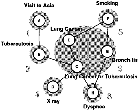
We demonstrate the usage of sensitivities on the well known Asia network [Lauritzen and Spiegelhalter, 1988] shown in Figure 3. The nodes in the network are: XA -"Visit to Asia", xn -"Tuberculosis, xc -"Lung Cancer or Tuberculosis", XD -"X-ray", XE -"Lung Cancer", XF -"Smoking", xc -"Bronchitis", XH -"Dyspnea". Tuberculosis and lung cancer are equally likely to cause shortness of breath (dyspnea), and are also equally likely to cause a positive chest X-ray. Bronchitis is another cause of dyspnea. Tu­ berculosis is more likely in people who have visited Asia. Smoking can cause lung cancer and bronchitis. The belief network describing this probabilistic model is given in Figure 3.

To convert the network to a multiply-valued node tree representation we combined nodes xc, XE, and xc in

Table 1: Prior Probability Distributions of Nodes in the Asia Network

Node	x o	x l	x 2	x 3	x 4	x s	x 6	x 7
x1 x2 x3	.9900 .9896 .5210 .8897	.0100 .0104 .4141 .1103	0	0	.0055	.0044	.0235	.0315

Table 2: Sensitivities between Adjacent Nodes in the Asia Network in QR-representation

one multiply-valued node X3. The six multiply-valued nodes are denoted by shadows on the background (all nodes but X3 remain binary). An instantiation of the node x2 divides the whole network into two, and an instantiation of the node x3 into four conditionally in­ dependent parts. The conditional probabilities for this network can be found in [Neapolitan, 1990]. The prob­ ability distributions and conditional probabilities for the multiply-valued nodes were computed using the LS algorithm and a perl script. The conditional probabil­ ities were converted to sensitivities using MATLAB. 5 Starting from this preprocessed information, the rest of the operations in the examples can be performed with a hand calculator.

The probability distributions for nodes X1 through X6 are given in Table 1. The states (columns) are enumer­ ated from zero, zero being the state where all nodes are false. Different states of the compound node are enumerated according to expression l::; 2i-1x;, where i is the position of a node from the right. Thus, for the compound node X3 = {xc,XE,XG} the ordering of states is C E G, C E G, . . . , C E G. From the table we can see that the probability of states X;i and X� is zero. Checking the conditional probabilities we find that indeed p( CIE) = 0 is zero and these states are im­ possible in a universe described by this belief network. Since their probability is always zero, we discard these states from further consideration. The sensitivities of the adjacent nodes in the QR-representation are given in Table 2. The information in Tables 1 and 2 com­ pletely describes the Asia network.

To illustrate our method we solve two practical prob­ lems. We perform probabilistic inference using node reduction ((6) and (13)), sensitivity reversal ((7) and

5The transformations used in Sections 4 and 5 were im­ plemented in MATLAB and are available upon request.

(14)), and update rule ((10) and (15)). We apply in­ cremental instantiation and update sensitivities and probability distributions between any two consecutive instantiations if necessary.

Example 1 From Table 1 we can see that among the general population about 1% visited Asia. What is the increase in this percentage for people with dyspnea?

The strategy to answer this query is to compute the binary sensitivity (Section 3.3) SHA and to convert it using (14) to the binary sensitivity SAH. The sensi­ tivity s61 of node x6 with respect to node xl is:

Since matrices R63 and Q32 contain only one row, the product R63QI2 is an inner product of two vectors of size six and, taking into account two zeros in the R63 matrix, it takes 4 multiplications and 3 summations to evaluate: R63QI2 = .5319. The product R32QI1 is an inner product of two vectors of size two and, taking into account the symmetric form of R32 and Q21, we evaluate: R32QI1 = .6726. For the binary sensitivity in the form (12), we get:

Now, we reverse the binary sensitivity S H A :

Rephrasing the result, the probability p(A) of the node XA changes by:::::; 5.8 x 10-4 each time when the proba­ bility p(H) of the node XH changes by one. If node XH is instantiated to true, the change in the probability

p(H) is �p(H) = p(H) = .5640 and the change in the probability p(A) of the node XA is:

Answer: The increase in the percentage is �p(xA) = 3.3 X 10 -2 % .

Example 2 A person visited Asia and has a positive chest X-ray result. What is the probability of dyspnea'?

We shall perform incremental instantiation with the first.

set { XA, XD }. We choose to instantiate node XA Using (6), we calculate 83 1 , 84 1 , and 861 (see the pre­ vious example):

The change in the probability distribution of the node X1 after instantiation is � p 1 = ( -.9900 .9900)T. Multiplying the sensitivity matrices by the change in the probability distribution of the node X 1 gives the changes in the probability distribution of nodes X3, X4, and X6. Adding the changes to the probability distributions in Table 1, we get:

Now we have to reverse the sensitivity 843 and to in­ stantiate node X4. The product Q43(A� 1 ))- 1 is the Q43 matrix with every element divided by the corre­ sponding probability from the probability distribution p(1 ) . 4 .

The multiplication by (I -�E) on the right is equiv­ alent to subtracting an arithmetic average (-1.170 + 6.892)/2 = 2.861 from both elements:

Reversing R43 to Q��) requires a little more work, but not much: the product R43A� 1 ) is the R43 matrix with every element multiplied by the corresponding probability from the probability distribution P�1\ the product R43P� 1 ) is the sum of all elements of the pre­ vious result and equals -.7423, and, as a reader can check, the final result can be expressed as (Q�Q), = (( � 3) p + .7423)((P � 1) )T),. The computation gives:

If the node XD is instantiated to true, the change in the probability pCl)(D) is �p(l)(D) = pCl)(D) = .8549 and the posterior probability pC2>(H) is:

Answer: The probability of dyspnea is p(2)(H) = .68.

DISCUSSION

Sensitivities provide a simple and intuitive description of the dependencies in a belief network. The term sen­ sitivity has been used before in a number of ways, but never in a way formal enough to show that probabilis­ tic inference can be performed based on sensitivities alone. Two definitions that are close in spirit to ours are in [Laskey, 1993], where sensitivity is a derivative of a target probability with respect to network parame­ ters, and in decision analysis [Howard, 1990], where the sensitivity describes the dependence of the expected value of the utility function on the input parameters to a probabilistic model. There have been other defi­ nitions of sensitivity as well [Pearl, 1988]. In our paper sensitivity is a linear transformation from the change in the probability of one node to the change in the probability of another node. The change can be due to the change in the network parameters, a change in the input parameters, or instantiations.

A belief network can be described in terms of sensi­ tivities between nodes and probability distributions of the nodes. Since the transformation from this rep­ resentation to the traditional representation in terms of conditional probabilities and back is a one-one re­ lation, both representations have the same expressive power. A person thinking in terms of probabilities asks the question "What is the probability of an event if certain facts are true?" A person thinking in terms of sensitivities asks "How does the probability distri­ bution change if some facts change?" Given the trans­ formation rules in this paper, these two questions are identical. We have shown how to make probabilistic inference based on sensitivities only, without ever con­ verting them back to conditional probabilities. Each node updates its own probability distribution based on the messages it receives from neighbors. In doing so it is not necessary to propagate messages throughout the whole network if we are concerned only with nodes in some localized part of the network.

Sensitivity is a very efficient and powerful repre­ sentation of dependencies. For binary nodes the node reduction is more than eight times more effi­ cient. For multiply-valued nodes the efficiency de­ pends on the rank of the probability matrix. The com­ putational complexity changes from 0 (IX;IIXiiiXkl) to O((IXil + I X k l ) x rank(8;j) x rank(8jk)) for the node reduction and from 0 (IX;IIXj I) to 0 ( (IX; I + I Xi I) x rank(8ij)) for the arc reversal. We believe that for the compound nodes obtained after

the conversion of an arbitrary network to a tree net­ work, the sensitivity matrices should have a low rank (see discussion at the end of Section 3.1).

One might argue that the efficiency of the operations with sensitivities is a result of the work done in trans­ forming conditional probabilities to sensitivities. In fact, this is exactly the result we want to achieve, i.e. to represent a belief network in a form that is conve­ nient for probabilistic inference. This representation can be computed once and then reused any number of times to evaluate different queries. The step of conversion from conditional probabilities to sensitiv­ ities is not absolutely necessary either: the learning algorithms that construct belief networks can be eas­ ily changed to train sensitivities instead of conditional probabilities.

Finally, although even approximate probabilistic in­ ference is NP-hard for general belief networks [Dagum and Luby, 1993], in Section 3.3 we showed that for a certain class of belief networks approximate probabilis­ tic inference with the exact upper bound on the error of the result can be performed in time independent of the size of the network. In fact, sensitivities open a path to a whole class of approximate algorithms. Given a belief network BN in tree representation we can build a belief network BN(r) where r is the maxi­ mum rank among all sensitivity matrices. Using linear algebra methods we can first remove those dependen­ cies from the sensitivity matrices which don't affect the joint probability distribution much, thus reducing r. The computation time for inference will decrease linearly with r, while the precision will have a weaker dependence provided that r is close to the original maximum rank.

On the whole, we believe that the concept of sensitivity is useful for probabilistic inference in belief networks. The reader is also referred to [Kozlov and Singh, 1995] for a more comprehensive treatment in which we build our theory beginning with a very simple case.

Acknowledgements

We thank the reviewers for valuable comments. We also thank Steve Hanks and Bruce D'Ambrosio for answering our many questions, Ross Shachter, Greg Provan, and Malcolm Pradhan for discussions, Adam Galper for his implementation of the LS algo­ rithm, John Hennessy for his support and guidance, and ARPA for financial support under contract no. N00039-91-C-0138.

References

Campbell, A. N. (1982). Recognition of a hidden min­ eral deposit by an artificial intelligence program. Sci­ ence, 217:927- 929.

Cooper, G. (1990). The computational complexity of probabilistic inference using Bayesian belief networks.

Artificial Intelligence, 42:393 - 405.

Dagum, P. and Luby, M. (1993). Approximating prob­ abilistic inference in Bayesian belief networks is NP­ hard. Artificial Intelligence, 60:141- 153.

Howard, R. A. (1990). From influence to relevance to knowledge. In Oliver, R. M. and Smith, J. Q., editors, Influence Diagrams, Belief Nets, and Decision Analy­ sis, pages 3 - 23. John Wiley & Sons, New York.

Kozlov, A. V. and Singh, J. P. (1995). Approxi­ mate probabilistic inference in Bayesian belief net­ works based on sensitivities. in preparation.

Laskey, K. B. (1993). Sensitivity analysis for prob­ ability assessment in Bayesian networks. In Hecker­ man, D. E., editor, Uncertainty in Artificial Intelli­ gence: Proceedings of the Ninth Conference, pages 136 - 142. Morgan Kaufmann.

Lauritzen, S. S. and Spiegelhalter, D. J. (1988). Lo­ cal computations with probabilities on graphical struc­ tures and their application to expert systems. Journal of the Royal Statistical Society, B 50:253 - 258.

Li, Z. and D'Ambrosio, B. (1994). Efficient infer­ ence in Bayes networks as a combinatorial optimiza­ tion problem. International Journal of Approximate Reasoning, 11(1):55- 81.

Middleton, B., Shwe, M. A., Heckerman, D. E., Hen­ rion, M., Horvitz, E. J., Lehmann, H. P., and Cooper, G. F. (1991). Probabilistic diagnosis using a reformu­ lation of the INTERNIST-1/QMR knowledge base. II. Evaluation of diagnostic performance. Methods of In­ formation in Medicine, 30( 4) :256 - 267.

Neapolitan, R. E. (1990). Probabilistic Reasoning in Expert Systems: Theory and Algorithms, page 279. John Wiley & Sons, New York.

Pearl, J. ( 1988). Probabilistic Reasoning in Intelligent Systems: Networks of Plausible Inference. Morgan Kaufmann.

Shachter, R. D. (1986). Evaluating influence diagrams. Operations Research, 34(6):871 - 882.

Shachter, R. D. (1991). A graph-based method for conditional independence. In D'Ambrosio, B., Smeth, P., and Bonissone, P., editors, Uncertainty in Artificial Intelligence: Proceedings of the Seventh Conference, pages 353- 360. Morgan Kaufmann.

Shortliffe, E. H. (1976). Computer-Based Medical Consultations: MYCIN. Elsvier-North Holland, New York.

Shwe, M. A., Middleton, B., Heckerman, D. E., Hen­ rion, M., Horvitz, E. J., Lehmann, H. P., and Cooper, G. F. (1991). Probabilistic diagnosis using a refor­ mulation of the INTERNIST-1/QMR knowledge base. I. The probabilistic model and inference algorithms. Methods of Information in Medicine, 30(4):241- 255.