Set Intersection and Consistency in Constraint Networks

Yuanlin Zhang

Department of Computer Science, Texas Tech University Lubbock, TX 79414 USA

Roland H. C. Yap

Department of Computer Science, National University of Singapore 3 Science Drive 2, Singapore 117543

Abstract

In this paper, we show that there is a close relation between consistency in a constraint network and set intersection. A proof schema is provided as a generic way to obtain consistency properties from properties on set intersection. This approach not only simplifies the understanding of and unifies many existing consistency results, but also directs the study of consistency to that of set intersection properties in many situations, as demonstrated by the results on the convexity and tightness of constraints in this paper. Specifically, we identify a new class of tree convex constraints where local consistency ensures global consistency. This generalizes row convex constraints. Various consistency results are also obtained on constraint networks where only some , in contrast to all in the existing work, constraints are tight.

1. Introduction

A constraint network consists of a set of variables over finite domains and a system of constraints over those variables. An important task is to find an assignment for all the variables such that all the constraints in the network are satisfied. If such an assignment exists, the network is satisfiable or globally consistent , and the assignment is called a solution. The problem of determining the global consistency of a general constraint network is NPcomplete. Usually a search procedure is employed to find a solution. In practice, due to efficiency considerations, the search is usually equipped with a filtering algorithm that prunes values of a variable or the combinations of values of a certain number of variables that cannot be part of any solution. The filtering algorithm can make a constraint network locally consistent in the sense that a consistent assignment of some variables can always be extensible to a new variable. An important and interesting question on local consistency is:

Is the local consistency obtained sufficient to determine the global consistency of the network without further search? As the filtering algorithm is of polynomial complexity, a positive answer would mean that the network can be solved in polynomial time.

Much work has been done to explore the relationship between local and global consistency in particular and the properties of local consistency in general. One direction is to make use of the topological structure of a constraint network. A classical result is that when the graph of a constraint network is a tree, arc consistency of the network is sufficient to ensure its global consistency (Freuder, 1982).

[email protected] [email protected]

Zhang & Yap

The second direction 1 makes use of semantic properties of the constraints. For monotone constraints , path consistency implies global consistency (Montanari, 1974). Van Beek and Dechter (1995) generalize monotone constraints to a larger class of row convex constraints . Dechter (1992) shows that a certain level of consistency in a constraint network whose domains are of limited size ensures global consistency. Later, Van Beek and Dechter (1997) study the consistency of constraint networks with tight and loose constraints.

The existing work along the two approaches has used specific and different techniques to study local and global consistency. In particular, there is little commonality in the details of the existing work. In much of the existing work, the techniques and consequently the proofs given are developed specifically for the results concerned.

In this paper, we show how much of this work can be connected together through a new approach to studying consistency in a constraint network. We unite two seemingly disparate areas: the study of set intersection on special sets and the study of k -consistency in constraint networks. In fact, k -consistency can be expressed in terms of set intersection, which allows one to obtain relationships between local and global consistency in a constraint network through the properties of set intersection on special sets. The main result of this approach is a proof schema that can be used to lift results from set intersection, which are rather general, to particular consistency results on constraint networks. One benefit of the proof schema lies in that it provides a modular way to greatly simplify the understanding and proofs of consistency results. This benefit is considerable as often the proofs of many existing results are complex and 'hard-wired'. Using this new approach, we show that it is precisely the various properties of set intersection that are the key to those results. Furthermore, the proofs become mechanical.

The following sketch illustrates briefly the use of our approach. One property of set intersection is that if the intersection of every pair ( 2 ) of tree convex sets (see Section 3) is not empty, the intersection of the whole collection of these sets is not empty too. From this property, we can see that the local information on the intersection of every pair of sets gives rise to the global information on the intersection of all sets. Intuitively, this relationship between the local and global information corresponds to obtaining global consistency from local consistency. The proof schema is used to lift the result on tree convex sets to the following consistency result. For a binary constraint network of tree convex constraints, ( 2 +1)-consistency (path consistency) implies global consistency of the network.

The usefulness of our new set-based approach is twofold. Firstly, it gives a clear picture of many of the existing results. For example, many well known results in the second direction based on semantic properties of the constraints (including van Beek & Dechter, 1995, 1997), as well as results from the first direction, can be shown with easy proofs that make use of set intersection properties. Secondly, by directing the study of consistency to that of set intersection properties, it helps improve some of the existing results and derive new results as demonstrated in sections 5-7.

This paper is organized as follows. In Section 2, we present necessary notations and concepts. In Section 3, we focus on properties of the intersection of tree convex sets and sets

1. There is a difference between the work concerned here and that studying the tractability of constraint languages (e.g., Schaefer, 1978; Jeavons, Cohen, & Gyssens, 1997). The latter considers the problems whose constraints are from a fixed set of relations while the former studies constraint networks with special properties .

with cardinality restrictions. In Section 4, we develop a characterization of k -consistency utilizing set intersection and the proof schema that offers a generic way to obtain consistency results from set intersection properties. The power of the new approach is demonstrated by new consistency results on the convexity and tightness of constraints. Tree convex constraints are studied in Section 5. On a constraint network of tree convex constraints, local consistency ensures global consistency, as a result of the intersection property of tree convex sets. The tightness of constraints is studied in Section 6. Thanks to the intersection properties of sets with cardinality restriction, a relation between local and global consistency is identified on weakly tight constraint networks in Section 6.1. These networks require only some, rather than all, constraints to be m -tight, improving the tightness result by van Beek and Dechter (1997). With the help of relational consistency, we show that global consistency can be achieved through local consistency on weakly tight constraint networks in Section 6.2. This type of result on tightness was not known before. In Section 6.3, we explore when a constraint network is weakly m-tight and present several results about the number of tight constraints sufficient or necessary for a network to be weakly tight. To make full use of the tightness of the constraints in a network, we propose dually adaptive consistency in Section 6.4. Dually adaptive consistency of a constraint network is determined by its topology and the tightest relevant constraint on each variable. For completeness, we include in Section 7 results on tightness and tree convexity that are based on relational consistency. We conclude in Section 8.

2. Preliminaries

/negationslash

A constraint network R is defined as a set of variables N = { x 1 , x 2 , . . . , x n } ; a set of finite domains D = { D 1 , D 2 , . . . , D n } where domain D i , for all i ∈ 1 ..n , is a set of values that variable x i can take; and a set of constraints C = { c S 1 , c S 2 , . . . , c S e } where S i , for all i ∈ 1 ..e , is a subset of { x 1 , x 2 , . . . , x n } and each constraint c S i is a relation defined on the domains of all variables in S i . Without loss of generality, we assume that, for any two constraints c S i , c S j ∈ C ( i = j ), S i = S j . The arity of constraint c S i is the number of variables in S i . For a variable x , D x denotes its domain. In the rest of this paper, we will often use network to mean constraint network.

/negationslash

An instantiation of variables Y = { x 1 , . . . , x j } is denoted by ¯ a = ( a 1 , . . . , a j ) where a i ∈ D i for i ∈ 1 ..j . An extension of ¯ a to a variable x ( / ∈ Y ) is denoted by (¯ a, u ) where u ∈ D x . An instantiation of a set of variables Y is consistent if it satisfies all constraints in R that do not involve any variables outside Y .

A constraint network R is k-consistent if and only if for any consistent instantiation ¯ a of any distinct k -1 variables, and for any new variable x , there exists u ∈ D x such that (¯ a, u ) is a consistent instantiation of the k variables. R is strongly k -consistent if and only if it is j -consistent for all j ≤ k . A strongly n -consistent network is called globally consistent .

For more information on constraint networks and consistency, the reader is referred to the work by Mackworth (1977), Freuder (1978) and Dechter (2003).

3. Properties on Set Intersection

In this section, we develop a number of set intersection results that will be used later to derive results on consistency. The set intersection property that we are concerned with is:

Given a collection of l finite sets, under what conditions is the intersection of all l sets not empty?

Here, we are particularly interested in the intersection property on sets with two interesting and useful restrictions: convexity and cardinality.

3.1 Tree Convex Sets

Given a collection of sets, some structures can be associated with the elements of the sets such that we can obtain interesting and useful set intersection results. Here we study the sets whose elements form a tree. We first introduce the concept of a tree convex set.

Definition 1 Given a discrete set U and a tree T with vertices U , a set A ⊆ U is tree convex under T if there exists a subtree of T whose vertices are A .

A subtree of a tree T is a subgraph of T that is a tree. Next we define when we can say a collection of sets are tree convex.

Definition 2 Given a collection of discrete sets S , let the union of the sets of S be U . The sets of S are tree convex under a tree T on U if every set of S is tree convex under T .

A collection of sets are said tree convex if there exists a tree such that the sets in the collection are tree convex under the tree.

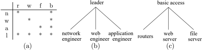
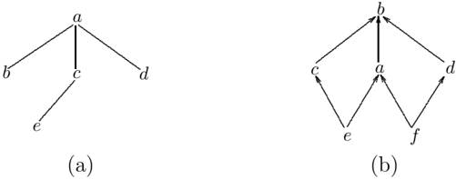
Example 1 Consider a set U = { a, b, c, d, e } and a tree given in Figure 1. The subset { a, b, c, d } is tree convex under the given tree. So is the set { b, a, c, e } since the elements of the set are a subtree. However, { b, c, e } is not tree convex as its elements do not form a subtree of the given tree.

Example 2 Consider S = {{ 1 , 9 } , { 3 , 9 } , { 5 , 9 }} . If we construct a tree on { 1 , 3 , 5 , 9 } with 9 being the root and 1 , 3 , 5 being its children, each set of S covers the nodes of exactly one branch of the tree. Hence, the sets of S are tree convex.

Tree convex sets have the following intersection property.

/negationslash

Lemma 1 (Tree Convex Sets Intersection) Given a finite collection of finite sets S , assume the sets of S are tree convex. ⋂ E ∈ S E = ∅ iff for all E 1 , E 2 ∈ S , E 1 ⋂ E 2 = ∅ .

/negationslash

Proof. Let l be the number of sets in S , and T a tree such that, for each E i ∈ S , E i is the vertices of a subtree T i of T . Assuming T is a rooted tree, every T i ( i ∈ 1 ..l ) is a rooted tree whose root is exactly the node nearest to the root of T . Let r i denote the root of T i for i ∈ 1 ..l .

/negationslash

To prove ⋂ i ∈ 1 ..l E i = ∅ , we want to show the intersection of the trees { T i | i ∈ 1 ..l } is not empty. The following propositions on subtrees are necessary in our main proof.

Proposition 1 Let T 1 , T 2 be two subtrees of a tree T , and T = T 1 ∩ T 2 . T is a tree.

/negationslash

If T = ∅ , it is a trivial tree. Now let T = ∅ . Since T is a portion of T 1 , there is no circuit in it. It is only necessary to prove T is connected. That is to show, for any two nodes u, v ∈ T , there is a path between them. u, v ∈ T 1 and u, v ∈ T 2 respectively imply that there exist paths P 1 : u, . . . , v in T 1 and P 2 : u, . . . , v in T 2 respectively. Recall that there is a unique path from u to v in T and that T 1 and T 2 are subtrees of T . Therefore, P 1 and P 2 cover the same nodes and edges, and thus they are in T , the intersection of T 1 and T 2 . P 1 is the path we want.

Proposition 2 Let T 1 , T 2 be two subtrees of a tree T , and T = T 1 ∩ T 2 . T is not empty if and only if at least one of the roots of T 1 and T 2 is in T .

/negationslash

Let r 1 and r 2 be the roots of T 1 and T 2 respectively. If r 1 ∈ T , the proposition is correct. Otherwise, we show r 2 ∈ T . Assume the contrary r 2 / ∈ T . Clearly, r 1 = r 2 . Let r be the first common ancestor of r 1 and r 2 and v the root of T ( T is a tree by Proposition 1). We have paths P 1 : r 1 , . . . , v in T 1 ; P 2 : r 2 , . . . , v in T 2 ; and P 3 : r, . . . , r 1 , and P 4 : r, . . . , r 2 in T . Since v is a descendant of both r 1 and r 2 , P 1 and P 2 share only the vertex v . Since r is the first common ancestor of r 1 and r 2 , P 3 and P 4 share only the vertex r . It can also be verified that P 3 and P 1 share only r 1 , P 2 and P 4 share only r 2 , and no vertex is shared by either P 1 and P 4 or P 2 and P 3 . Hence, the closed walk P 3 P 1 P ′ 2 P ′ 4 , where P ′ 2 and P ′ 4 are the reverse of P 2 and P 4 respectively, is a simple circuit. It contradicts that there is no circuit in T .

Further, we have the following observation.

Proposition 3 Let T be a tree with root r , and T 1 and T 2 two subtrees of T with roots r 1 and r 2 respectively. Let r 1 be not closer to r than r 2 , and T the intersection of T 1 and T 2 . r 1 is the root of T if T is not empty.

The proposition is true if r 1 = r 2 . Now let r 1 be farther to r than r 2 . Clearly r 2 / ∈ T 1 and thus r 2 / ∈ T . By Proposition 2, r 1 is the root of T .

/negationslash

T 1 , T 2 , . . . , T l such that its root r max is the farthest away from r of T among the roots of

Let T = ⋂ i ∈ 1 ..l T i . We are ready now to prove our main result T = ∅ . Select a tree T max from

the concerned trees. In accordance with Proposition 3, that T max intersect with every other tree implies that r max is a node of every T i ( i ∈ 1 ..l ). Therefore, r max ∈ T . ✷

Remark. A partial order can be represented by an acyclic directed graph. It is tempting to further generalize tree convexity to partial convexity in the following way.

Given a set U and a partial order on it, a set A ⊂ U is partially convex if and only if A is the set of nodes of a connected subgraph of the partial order. Given a collection of sets S , let the union of the sets of S be U . The sets of S are partially convex if there is a partial order on U such that every set of S is partially convex under the partial order.

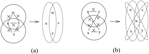
However, with this generalization, we can not get a result similar to Lemma 1, which is illustrated by the following example. Consider three sets { c, b, d } , { d, f, a } and { a, e, c } that are the nodes of the diagram given in Figure 1(b). These sets are partially convex and intersect pairwise. However, the intersection of all three sets is empty.

3.2 Sets with Cardinality Restrictions

Another useful restriction that we will place on sets is to restrict their cardinalities. As a special case, consider a set with only one element a . If its intersection with every other set is not empty, we are able to conclude that every set contains a , and thus the intersection of all the sets is not empty. Generally, if a set has at most m elements, we have the following result.

Lemma 2 Consider a finite collection of l sets S = { E 1 , E 2 , . . . , E l } and a number m < l . Assume one set E 1 ∈ S has at most m elements.

/negationslash

iff the intersection of E 1 and any other m sets of S is not empty.

Proof. The necessary condition is immediate.

To prove the sufficient condition, we show that the intersection of E 1 and any other k ( m ≤ k ≤ l -1) sets of S is not empty by induction on k . When k = m , the lemma is true according to its assumption. Assuming that the intersection of E 1 and any other k -1 ( ≥ m ) sets of S is not empty, we show that the intersection of E 1 and any other k sets of S is not empty. Without loss of generality, the subscripts of the k sets are numbered from 2 to k +1. For 2 ≤ i ≤ k +1, let A i be the intersection of E 1 and the k sets except E i :

First, we show by contradiction that there exist some i, j ∈ 2 ..k + 1 , i = j such that A i ∩ A j = ∅ . Assume A i ∩ A j = ∅ for all distinct i and j . According to the construction of A i 's,

/negationslash

/negationslash

and | A i | ≥ 1 by the induction assumption. Hence,

/negationslash which contradicts | E 1 | ≤ m .

/negationslash

✷

This lemma leads to the following corollary where the intersection of every m +1 sets is not empty.

Corollary 1 (Small Set Intersection) Consider a finite collection of l sets S and a number m<l . Assume one set of S has at most m elements.

/negationslash

iff the intersection of any m +1 sets of S is not empty.

There are other specialized versions (Zhang & Yap, 2003) of Lemma 2 on which some existing works by van Beek and Dechter (1997) and David (1993) are based.

When the sets of concern have a cardinality larger than a certain number, the intersection of these sets is not empty under some conditions. The reader may refer to the Large Sets Intersection lemma (Zhang & Yap, 2003) for more details.

4. Set Intersection and Consistency

In this section, we first relate consistency in constraint networks to set intersection. Using this result, we present a proof schema that allows us to study the relationship between local and global consistency from the properties of set intersection.

Underlying the concept of k -consistency is whether an instantiation of some variables can be extended to a new variable such that all relevant constraints on the new variable are satisfied. A relevant constraint on a variable x i with respect to Y is a constraint that contains only x i and some variables of Y . Given an instantiation of Y , each relevant constraint allows a set (possibly empty) of values for the new variable. We call this set an extension set . The satisfiability of all relevant constraints depends on whether the intersection of their extension sets is non-empty (see Lemma 3).

Definition 3 Given a constraint c S i , a variable x ∈ S i , and any instantiation ¯ a of S i -{ x } , the extension set of ¯ a to x with respect to c S i is defined as

An extension set is trivial if it is empty; otherwise it is non-trivial .

Since A i ∩ A j = ∅ for some i, j ∈ 2 ..k +1 , i = j ,

/negationslash

Recall that D x refers to the domain of variable x . Throughout the paper, it is often the case that an instantiation ¯ a of S - { x } is already given, where S - { x } is a superset of S i - { x } . Let ¯ b be the instantiation obtained by restricting ¯ a to the variables only in S i -{ x } . For ease of presentation, we continue to use E i,x (¯ a ), rather than E i,x ( ¯ b ), to denote the extension of ¯ b to x under constraint c S i . To make the presentation easy to follow, some of the three parameters i , ¯ a , and x may be omitted from an expression hereafter whenever they are clear from the context. For example, given an instantiation ¯ a and a new variable x , to emphasize different extension sets with respect to different constraints c S i , we write E i instead of E i,x (¯ a ) to simply denote an extension set.

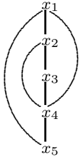
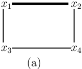
Example 3 Consider a network with variables { x 1 , x 2 , x 3 , x 4 , x 5 } :

Let ¯ a = ( a, b, a ) be an instantiation of variables Y = { x 1 , x 2 , x 4 } . The relevant constraints to x 3 are c S 1 , c S 2 , and c S 3 . c S 4 is not relevant since it contains x 5 outside Y . The extension sets of ¯ a to x 3 with respect to the relevant constraints are:

The intersection of the extension sets above is not empty, implying that ¯ a can be extended to satisfy all relevant constraints c S 1 , c S 2 and c S 3 .

Let ¯ a = ( b, c ) be an instantiation of { x 2 , x 3 } . E 1 ,x 1 (¯ a ) = ∅ and thus it is trivial. In other words, with a trivial extension set, an instantiation can not be extended to satisfy the constraint of concern.

The relationship between k-consistency and set intersection is characterized by the following lemma.

Lemma 3 (Set Intersection and Consistency; Lifting) A constraint network R is k -consistent if and only if for any consistent instantiation ¯ a of any ( k -1) distinct variables Y = { x 1 , x 2 , . . . , x k -1 } , and any new variable x k ,

/negationslash

where E i j is the extension set of ¯ a to x k with respect to c S i j , and c S i 1 , . . . , c S i l are all relevant constraints.

Proof. It follows directly from the definition of k -consistency in Section 2 and the definition of extension set. ✷

The insight behind this lemma is to examine consistency from the perspective of set intersection.

Example 4 Consider again Example 3. We would like to check whether the network is 4 -consistent. Consider the instantiation ¯ a of Y again. This is a trivial consistent instantiation since the network doesn't have a constraint among the variables in Y . To extend it to x , we need to check the first three constraints c S 1 to c S 3 . The extension is feasible because the intersection of E 1 , E 2 , and E 3 is not empty. We show the network is 4 -consistent, by exhausting all consistent instantiations of any three variables. Conversely, if we know the network is 4 -consistent, we can immediately say that the intersection of the three extension sets of ¯ a to x is not empty.

The usefulness of this lemma is that it allows consistency information to be obtained from the intersection of extension sets, and vice versa. With this point of view of consistency as set intersection, some results on set intersection properties, including all those in Section 3, can be lifted to get various consistency results for a constraint network through the following proof schema .

Proof Schema

1. ( Consistency to Set ) From a certain level of consistency in the constraint network, we derive information on the intersection of the extension sets by Lemma 3.
2. ( Set to Set ) From the local intersection information of sets, information may be obtained on intersection of more sets.
3. ( Set to Consistency ) From the new information on intersection of extension sets, higher level of consistency is obtained by Lemma 3.
4. ( Formulate conclusion on the consistency of the constraint network ). ✷ In the proof schema, step 1 (consistency to set), step 3 (set to consistency), and step 4 are straightforward in many cases. So, Lemma 3 is also called the lifting lemma because once we have a set intersection result (step 3), we can easily have consistency results on a network (step 4). The proof schema establishes a direct relationship between set intersection and
5. consistency properties in a constraint network.

In the following sections, we demonstrate how the set intersection properties and the proof schema are used to obtain new results on the consistency of a constraint network.

5. Global Consistency of Tree Convex Constraints

The notion of extension set plays the role of a bridge between the restrictions to set(s) and properties of special constraints. In this section, we consider the constraints arising from tree convex sets (Lemma 1). A constraint is tree convex if all the extension sets with respect to the constraint are tree convex.

Definition 4 A constraint c S is tree convex with respect to x i and a tree T i on D i if and only if the sets in

are tree convex under T i . A constraint c S is tree convex under a tree T on the union of the domains of the variables in S , if it is tree convex with respect to every x ∈ S under T .

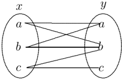
Example 5 Tree convex constraints can occur where there is a relationship among the values of a variable. Consider the constraint on the accessibility of a set of facilities by a

set of persons. The personnel include a network engineer, web server engineer, application engineer, and a team leader. The relationship among the staff is that the team leader manages the rest, which forms a tree structure shown in Figure 2(b). There are different accessibilities to a system which includes basic access, access to the network routers, access to the web server, and access to the file server. In order to access the routers and servers, one has to have the basic access right, implying a tree structure (Figure 2(c)) on the access rights. The constraint is that the team leader is able to access all the facilities while each engineer can access only the corresponding facility (e.g., the web server engineer can access the web server). This tree convex constraint is shown in Figure 2(a) where the rows are named by the initials of the engineers and the columns by the initials of the access rights. The tree on the union of personnel and the accessibilities can be obtained from their respective trees (in Figure 2(b) and (c)) by adding an edge, say between web server and leader. Note that the constraint in Figure 2(a) is not row convex.

Example 6 Tree convex constraints can also be used to model some scene labeling problems naturally as shown by Zhang and Freuder (2004).

Definition 5 A constraint network is tree convex if there exists a tree T on the union of all its variable domains such that all constraints are tree convex under T .

Tree convex constraints generalize row convex constraints introduced by van Beek and Dechter (1995).

Definition 6 A constraint c S is row convex with respect to x if and only if the sets in

are tree convex under a tree where any node has at most one child. Such a tree is called a total ordering . A constraint c S is row convex if, under a total ordering on the union of the involved domains, it is row convex with respect to every x ∈ S .

Example 7 For the constraint c in Example 5 to be row convex, b (basic access) has to be the neighbor of r (routers), w (web server), and f (file server). However, in a total ordering, a value can be the neighbor of at most two other values. Hence, c is not row convex but is tree convex.

By the property of set intersection on tree convex sets and the proof schema, we have the following consistency results on tree convex constraints.

Theorem 1 (Tree Convexity) Let R be a network of constraints with arity at most r and strongly 2( r -1) + 1 consistent. If R is tree convex then it is globally consistent.

Proof. The network is strongly 2( r -1) + 1 consistent by assumption. We prove that the network is k consistent for any k ∈ { 2 r, . . . , n } .

Consider any instantiation ¯ a of any k -1 variables and any new variable x . Let the number of relevant constraints be l . For each relevant constraint, there is one extension set of ¯ a to x . So, we have l extension sets. If the intersection of all l sets is not empty, we have a value for x such that the extended instantiation satisfies all relevant constraints.

( Consistency to Set ) Consider any two of the l extension sets: E 1 and E 2 . The two corresponding constraints involve at most 2( r -1)+1 variables since the arity of a constraint is at most r and each of the two constraints has x as a variable. By the consistency lemma, that R is (2( r -1) + 1)-consistent implies that the intersection of E 1 and E 2 is not empty.

( Set to Set ) Since all relevant constraints are tree convex under the given tree, the extension sets of ¯ a to x are tree convex. Henceforth, the fact that every two of the extension sets intersect shows that the intersection of all l extension sets is not empty, by the tree convex sets intersection lemma.

( Set to Consistency ) From the consistency lemma, we have that R is k -consistent. ✷ Since a row convex constraint is tree convex, this result generalizes the consistency result on row convex constraints reported by van Beek and Dechter (1995). It is interesting to observe that the latter can be lifted from a set intersection results on convex sets (Zhang & Yap, 2003).

A question raised by Theorem 1 is how efficient it is to check whether a constraint network is tree convex. Yosiphon (2003) has proposed an algorithm to recognize a tree convex constraint network in polynomial time.

6. Consistency and the Tightness of Constraints

In this section, we will present various consistency results on the networks with m -tight constraints.

6.1 Global Consistency on Weakly Tight Networks

The tightness of constraints has been related to the consistency of a constraint network by van Beek and Dechter (1997). The m-tightness of a constraint is characterized by the cardinality of the extension sets in the following way.

Definition 7 (van Beek & Dechter, 1997) A constraint c S i is m-tight with respect to x ∈ S i iff for any instantiation ¯ a of S i -{ x } ,

A constraint c S i is m-tight iff it is m-tight with respect to every x ∈ S i .

Given an instantiation, if its extension set with respect to x is the same as the domain of variable x , i.e., | E i,x | = | D x | , the instantiation is supported by all values of x and thus easy to be satisfiable. Hence, in the definition above, these instantiations do not affect the m -tightness of a constraint.

Example 8 Consider the constraint c xy in Figure 3 where D x = D y = { a, b, c } . An edge in the graph denotes that its ends are allowed by c xy . It can be verified that for the values of x , their extension sets have a cardinality of 2 , and for values of y , their extension sets have a cardinality from 1 to 3 . Hence, c xy can be said 2-tight or 3-tight but not 1-tight.

We are specially interested in the following tightness.

Definition 8 A constraint c S i is properly m-tight with respect to x ∈ S i iff for any instantiation ¯ a of S i -{ x } ,

A constraint c S i is properly m-tight iff it is properly m-tight with respect to every x ∈ S i .

A constraint is m -tight if it is properly m -tight. The converse might not be true. For example, the constraint x ≤ y , where x ∈ { 1 , 2 , . . . , 10 } and y ∈ { 1 , 2 , . . . , 10 } , is 9-tight but not properly 9-tight. It is properly 10-tight since | E x (10) | = 10 when y = 10.

Next, we define a special constraint network which allows us to make a more accurate connection between the tightness of constraints and the consistency of the network.

Definition 9 A constraint network is weakly m-tight at level k iff for every set of variables { x 1 , x 2 , . . . , x l } ( k ≤ l < n ) and a new variable x , there exists a properly m -tight constraint among the relevant constraints on x with respect to { x 1 , x 2 , . . . , x l } .

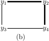
Example 9 The network in Figure 4(a) is weakly tight at level 3 because for any three variables and a fourth variable, one of the relevant constraints is properly m -tight. The network in Figure 4(b) is not weakly tight at level 3 since for { y 1 , y 3 , y 4 } and y 2 , none of the relevant constraints c y 1 y 2 and c y 4 y 2 is properly m -tight.

By the small set intersection corollary (Corollary 1), we have the following consistency result on a weakly m -tight network.

Theorem 2 (Weak Tightness) If a constraint network R with constraints of arity at most r is strongly (( m +1)( r -1)+1) -consistent and weakly m -tight at level (( m +1)( r -1)+1) , it is globally consistent.

Proof. Let j = ( m +1)( r -1)+1. The constraint network R will be shown to be k -consistent for all k ( j < k ≤ n ).

Let Y = { x 1 , . . . , x k -1 } be a set of any k -1 variables, and ¯ a be an instantiation of all variables in Y . Consider any additional variable x k . Without loss of generality, let the relevant constraints be c S 1 , . . . , c S l , and E i be the extension set of ¯ a to x k with respect to c S i for i ≤ l .

( Consistency to Set ) Consider any m +1 of the l extension sets. All the corresponding m + 1 constraints contain at most ( m + 1)( r -1) + 1 variables including x k . Since R is (( m +1)( r -1)+1)-consistent, by the set intersection and consistency lemma, the intersection of the m +1 extension sets is not empty.

( Set to Set ) The network is weakly m -tight at level (( m +1)( r -1) + 1). So, there must be a properly m -tight constraint among the relevant constraints c S 1 , . . . , c S l . Let it be c S i . We know its extension set | E i | ≤ m . Since the intersection of every m +1 of the extension sets is not empty, all l extension sets share a common element by the small set intersection corollary.

( Set to Consistency ) By the lifting lemma, R is k -consistent. ✷

In a similar fashion, the main tightness result by van Beek and Dechter (1997), where all the constraints are required to be m -tight, can be lifted from the small sets intersection corollary by Zhang and Yap (2003). This uniform treatment of lifting set intersection results to consistency results is absent from the existing works (e.g., Dechter, 1992; van Beek & Dechter, 1995, 1997; David, 1993).

The tightness result by van Beek and Dechter (1997) requires every constraint to be m -tight. The weak tightness theorem, on the other hand, does not require all constraints to be properly m -tight. The following example illustrates this difference.

Example 10 For a weakly m -tight network, we are interested in its topological structure. Thus we have omitted the domains of variables here. Consider a network with five variables labeled { 1 , 2 , 3 , 4 , 5 } . In this network, for any pair of variables and for any three variables, there is a constraint. Assume the network is already strongly 4 -consistent.

Since the network is already strongly 4 -consistent, we can simply ignore the instantiations with less than 4 variables. This is why we introduce the level at which the network is weakly m -tight. The interesting level here is 4 . Table 1 shows the relevant constraints for each possible extension of four instantiated variables to the other one. In the first row, 1234 → 5

Table 1: Relevant constraints in extending an instantiation of four variables to a new variable

Extension	Relevant constraints
1234 → 5,	125*,	135 ,	145 ,	235,	245,	345,	15+,	25 ,	35 ,	45
2345 → 1,	231 ,	241 ,	251*,	341,	351,	451,	21 ,	31 ,	41 ,	51+
3451 → 2,	132 ,	142 ,	152*,	342,	352,	452,	12 ,	32+,	42 ,	52
4512 → 3,	123 ,	143*,	153 ,	243,	253,	453,	13 ,	23+,	43 ,	53
5123 → 4,	124 ,	134*,	154 ,	234,	254,	354,	14 ,	24 ,	34+,	54

stands for extending the instantiation of variables { 1 , 2 , 3 , 4 } to variable 5 . Entries in its second column denote a constraint. For example, 125 denotes c 125 . If the constraints on { 1 , 2 , 5 } and { 1 , 3 , 4 } (suffixed by * in the table) are properly m -tight, the network is weakly m -tight at level 4 . Alternatively, if the constraints { 1 , 5 } , { 2 , 3 } and { 3 , 4 } (suffixed by +) are properly m -tight, the network will also be weakly m -tight. The tightness result by van Beek and Dechter (1997) requires all binary and ternary constraints to be m -tight.

6.2 Making Weakly Tight Networks Globally Consistent

Consider the weak tightness theorem in the previous section. Generally, a weakly m -tight network might not have the level of local consistency required by the theorem. It is tempting to enforce such a level of consistency on the network to make it globally consistent. However, this procedure may result in constraints with higher arity.

/negationslash

Example 11 Consider a network with variables { x, x 1 , x 2 , x 3 } . Let the domains of x 1 , x 2 , x 3 be { 1 , 2 , 3 } , the domain of x be { 1 , 2 , 3 , 4 } , and the constraints be that all the variables should take different values: x = x 1 , x = x 2 , x = x 3 , x 1 = x 2 , x 1 = x 3 , x 2 = x 3 . This network is strongly path consistent. In checking the 4-consistency of the network, we know that the instantiation (1 , 2 , 3) of { x 1 , x 2 , x } is consistent but can not be extended to x 3 . To enforce 4-consistency, it is necessary to introduce a ternary constraint on { x 1 , x 2 , x } to make (1 , 2 , 3) no longer a valid instantiation.

/negationslash

/negationslash

/negationslash

/negationslash

/negationslash

To make the new network globally consistent, the newly introduced constraints with higher arity may in turn require higher local consistency in accordance with Theorem 2. Therefore, it is difficult to predict an exact level of consistency (variable based) to enforce on the network to make it globally consistent.

In this section, relational consistency will be used to make a constraint network globally consistent.

Definition 10 (van Beek & Dechter, 1997) A constraint network is relationally m-consistent iff given (1) any m distinct constraints c S 1 , . . . , c S m , and (2) any x ∈ ∩ m i =1 S i , and (3) any consistent instantiation ¯ a of the variables in ( ∪ m i =1 S i - { x } ) , there exists an extension of ¯ a to x such that the extension is consistent with the m relations. A network is strongly relationally m -consistent if it is relationally j -consistent for every j ≤ m .

Variables are no longer of concern in relational consistency. Instead, constraints are the basic unit of consideration. Intuitively, relational m -consistency concerns whether all m constraints agree at every one of their shared variables. It makes sense because different constraints interact with each other exactly through the shared variables.

Relational 1-, and 2-consistency are also called relational arc, and path consistency, respectively.

Using relational consistency, we are able to obtain global consistency by enforcing local consistency on the network.

Proposition 4 The weak m -tightness at level k of a constraint network is preserved by the process of enforcing relational consistency on the network.

Proof. Let R be the constraint network before relational consistency enforcing and R 1 the network after consistency enforcing. Clearly, R and R 1 have the same set of variables. Consider any set of variables { x 1 , x 2 , . . . , x l } ( k ≤ l < n ) and a new variable x . Since R is weakly m -tight at level k , there exists a properly m -tight constraint c among the relevant constraints on x with respect to { x 1 , x 2 , . . . , x l } . Enforcing relational consistency on a constraint network will only tighten a constraint. So, the proper m -tightness of c is preserved. Hence, R 1 is weakly m -tight at level k . ✷

Now we have the main result of this subsection.

Theorem 3 A constraint network weakly m -tight at level ( m + 1)( r -1) + 1 , where r is the maximal arity of the constraints of the network, is globally consistent after it is made strongly relationally ( m +1) -consistent.

Proof. By Proposition 4, the network is still weakly m -tight at ( m +1)( r -1) + 1 after enforcing strong relational ( m + 1)-consistency on it. Let r 1 be the maximal arity of the constraints of the new network after consistency enforcing. Clearly, r 1 ≥ r . So, the network is m -tight at ( m +1)( r 1 -1) + 1 by Proposition 6. The theorem follows immediately from Theorem 8 in Section 7. ✷

The implication of this theorem is that as long as we have certain properly m -tight constraints on certain combinations of variables, the network can be made globally consistent by enforcing relational ( m +1)-consistency.

We have the following observation on the weak m -tightness of a network.

Proposition 5 A constraint network is weakly m -tight at any level if the constraint between every two variables in the network is properly m -tight.

Proof. Consider any level k , any set of variables Y = { x 1 , x 2 , . . . , x l } ( k ≤ l ≤ n ), and any new variable x / ∈ Y . Since the constraint between any two variables is properly m -tight, the constraint c { x 1 ,x } on x 1 and x is properly m -tight. Therefore, there is a properly m-tight constraint c { x 1 ,x } among the relevant constraints after an instantiation of Y . ✷

This observation shows that the proper m -tightness of the constraints on every two variables is sufficient to determine the level of local consistency needed to ensure global consistency of a constraint network.

Remark. Proposition 5 assumes there is a constraint between every two variables. If there is no constraint between some two variables, a universal constraint is introduced. In

this case, we can enforce path consistency on the constraint network to make the binary constraints tighter so that lower level of relational consistency is needed to make the network globally consistent.

6.3 Properties of Weakly Tight Constraint Networks

Since for a weakly m -tight constraint network global consistency can be achieved through local consistency, it is interesting and important to investigate the conditions for a network to be weakly m -tight. Although Proposition 5 shows a sufficient condition, it requires every binary constraint be tight. As we can see from Example 9(a), the required number of tight constraints for a constraint network to be weakly tight can be further reduced. This subsection is focused on the understanding of the relationship between the number of tight constraints and the weak tightness of a constraint network.

There is a strong relationship among different levels of weak tightness in a network.

Proposition 6 If a constraint network is weakly m -tight at level k for some m , it is weakly m -tight at any level j > k .

Proof. For any j > k , we prove that the network is weakly tight at level j . That is, for any set of variables Y = { x 1 , . . . , x j } ( k ≤ j < n ) and a new variable x , we show that there exists an m -tight relevant constraint on x with respect to Y . Since the network is weakly tight for k < j , there exists an m -tight relevant constraint on x with respect to a subset of Y . This constraint is still relevant on x with respect to Y , and thus the one we look for. ✷

In the following, we present two results on sufficient conditions for a constraint network to be weakly m -tight.

Theorem 4 Given a constraint network ( V, D, C ) and a number m , if for every x ∈ V , there are at least n -2 properly m -tight binary constraints on it, then the network is weakly m -tight at level 2 .

Proof. For any two variables { x, y } and a third variable z , the relevant constraints on z with respect to { x, y } are c xz and c yz . We know that the number of relevant binary constraints on z with respect to V is n -1. That n -2 of them are properly m -tight means either c xz or c yz must be properly m -tight. ✷

In fact, for the weak tightness at a higher level, we need fewer constraints to be m -tight as shown by the following result.

Theorem 5 A constraint network ( V, D, C ) is weakly m -tight at level k if for every x ∈ V , there are at least n -k properly m -tight binary constraints on it.

Proof. For any set Y of k variables and a new variable z , we show that there is a properly m -tight relevant constraint on z with respect to Y . Otherwise, none of the k binary constraints on z is properly m -tight. Since the total number of the relevant binary constraints on z is n -1, the number of properly m -tight binary constraints on z is at most ( n -1) -k , which contradicts that z is involved in n -k properly m -tight binary constraints. ✷

This result reveals that for a constraint network to be weakly tight at level k , it could need as few as n ( n -k +1) / 2 properly m -tight binary constraints, in contrast to the result in Theorem 3 where all binary constraints are required to be properly m -tight.

An immediate question is: What is the minimum number of m -tight constraints required for a network to be weakly tight? It can be answered by the following result on weak tightness at level 2.

Theorem 6 Given a number m , for a constraint network to be weakly m -tight at level 2 , it needs at least

m -tight binary or ternary constraints.

Proof. Given a network, its weak m -tightness at level 2 depends on the tightness of only binary and ternary constraints. Among all weakly m -tight (at level 3) constraint networks with n variables, let R 1 be the network that has a minimal set of properly m -tight binary and ternary constraints.

In the following exposition, a constraint is denoted by its scope. For example, we use { u, v, w } and { u, v } to denote ternary constraint c { u,v,w } and binary constraint c uv respectively. A constraint is non-properly-m-tight if it is not properly m -tight.

The proof consists of three steps.

Step 1. While preserving the weak m -tightness of R 1 and the number of properly m -tight constraints in R 1 , we modify, if necessary, the proper m -tightness of some constraints in R 1 such that, for any properly weak m -tight constraint { u, v, w } , none of the binary constraints { u, v } , { v, w } , and { u, w } is properly m -tight.

To modify the proper m -tightness of a constraint c in R 1 is to remove c from the network and introduce a new constraint on the same set of variables of c with the desirable proper m -tightness.

We claim that, for any properly m -tight constraint { u, v, w } , at most one of { u, v } , { v, w } , and { u, w } is properly m -tight. Otherwise, at least two of them are properly m -tight, which means { u, v, w } can be modified to be not properly m -tight, contradicting the minimality of the number of properly m -tight constraints in R 1 .

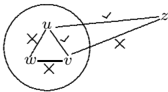
Assume { u, v } is properly m -tight. Since { u, v, w } is properly m -tight, there should be a reason for { u, v } to be properly m -tight. The only reason is that there exists another variable z such that one of { u, z } and { v, z } is not properly m -tight, and { u, v, z } is not properly m -tight, too. See Figure 5. Without loss of generality, let { u, z } be properly m -tight, implying that the constraint { v, z } is not properly m -tight. The constraint { z, v, w } is properly m -tight because { v, z } and { v, w } are not properly m -tight.

Now we modify the constraints { u, v, w } and { z, v, w } to be not properly m -tight and modify the constraints { z, v } and { v, w } to be properly m -tight. This modification preserves the number of properly m -tight constraints in R 1 and the weak m -tightness of R 1 .

Step 2. While preserving the weak m -tightness of R 1 and the number of properly m -tight constraints in R 1 , we next modify, if necessary, the proper m -tightness of the constraints in R 1 such that no two properly m -tight ternary constraints share any variables.

or otherwise

Case 1: Two properly m -tight constraints { u, v, w } and { u, v, z } share two variables { u, v } . See Figure 6(a). Since { w,u } and { u, z } are not properly m -tight (in terms of step 1), { w,u,z } has to be properly m -tight. Since { w,v } and { v, z } are not m -tight, { w,v, z } has to be m -tight.

We modify the four ternary constraints to be not properly m -tight and modify the four binary constraints { w,u } , { u, z } , { z, v } and { v, w } to be properly m -tight. This preserves the weak m -tightness of R 1 and the number of properly m -tight constraints in R 1 .

Case 2: Two properly m -tight constraints { u, v, w } , and { w,x,y } share one variable w . Since { u, w } and { w,x } are not properly m -tight, { u, w, x } has to be properly m -tight. Since { v, w } and { w,y } are not properly m -tight, { v, w, y } has to be properly m -tight. Similarly, { u, w, y } and { v, w, x } have to be properly m -tight. Now, if we modify the four binary constraints { u, w } , { w,x } , { v, w } , and { w,y } to be properly m -tight and the six ternary constraints to be non-properlym -tight, the new network is still weakly m -tight with fewer m -tight constraints. This contradicts the minimality of the number of properly m -tight constraints in R 1 . Hence, case 2 is not possible.

Step 3. As a result of the first two steps, in the network R 1 , the scopes of the properly m -tight ternary constraints are disjoint, and the binary constraint between any two variables of a properly m -tight ternary constraint is not properly m -tight.

Let B (and T respectively) be the set of the properly m -tight binary (and ternary respectively) constraints of R 1 .

Assume | T | = k . Since it is difficult to count B , we count the maximum number of non-properlym -tight binary constraints in R 1 . We have 3 k non-properlym -tight binary constraints due to T . We should not have any non-properlym -tight binary constraints between a variable in T and a variable outside T . Let V ′ be the variables outside T . We have | V ′ | = n -3 k . The other non-properlym -tight constraints fall only between variables in V ′ . Since R 1 is weakly tight at level 2, there is no two non-properlym -tight constraints on any variable in V ′ . Hence, there are at most ( n -3 k ) / 2 non-properlym -tight constraints if n -3 k is even, and otherwise at most ( n -3 k -1) / 2 ones. So the number, denoted by δ , of the properly m -tight constraints in R 1 would be the sum of the cardinality of T and B :

The fact that δ is minimal implies that k should be maximized. If n is a multiple of 3, the number of properly m -tight constraints is n ( n -1) / 2 -2 n/ 3; if n is 1 more than a multiple of 3, the number is n ( n -1) / 2 -2( n -1) / 3; otherwise the number is ( n -1)(3 n -1) / 6. ✷

This result shows that under the concept of k -consistency we still need a significant number of constraints to be properly m -tight to predict the global consistency of a network in terms of constraint tightness.

6.4 Dually Adaptive Consistency

A main purpose of our characterization of weak m -tightness of a network is to help identify a consistency condition under which a solution of a network can be found without backtracking, i.e., efficiently. We have studied constraint tightness under the concept of k -consistency in the previous subsections. In this subsection, we introduce dually adaptive consistency to achieve backtrack free search by taking into account both the tightness of constraints and the topological structure of a network.

The idea of adaptive consistency (Dechter & Pearl, 1987) is to enforce only the necessary level of consistency on each part of a network to ensure global consistency. It assumes an ordering on the variables. For any variable x , it only requires that a consistent instantiation of the relevant variables before x can be consistently extensible to x . Other variables do not play any direct role on x and thus are ignored when dealing with x .

We first introduce some notations used in adaptive consistency.

The width of a variable with respect to a variable ordering is the number of constraints involving x and only variables before x . See Figure 7 for an example.

Given a network, a variable ordering, and a variable x , the directionally relevant constraints on x are those involving x and only variables before x . In the following, DR ( x ) is used to denote the directionally relevant constraints on x , and S used to denote all variables occurring in the constraints of DR ( x ).

The constraints of DR ( x ) are consistent on x if and only if, for any consistent instantiation ¯ a of S - { x } , there exists u ∈ D x such that (¯ a, u ) satisfies all the constraints of DR ( x ).

We next define the adaptive consistency of a network.

Definition 11 Given a constraint network and an ordering on its variables, the network is adaptively consistent if and only if for any variable x , its directionally relevant constraints are consistent on x .

The adaptive consistency is presented as an algorithm by Dechter (2003) although, for the purpose of this paper, we prefer a declarative characterization.

For an adaptively consistent network, a solution can be found without backtracking.

Proposition 7 Given a constraint network and an ordering on its variables, a backtrack free search is ensured if the network is adaptively consistent.

Proof. Assume we have found a consistent instantiation of the first k variables (in terms of the given ordering). They can be consistently extended to x k +1 because all directionally relevant constraints on x k +1 are consistent on x k +1 . ✷

When a network is not adaptively consistent, the algorithm by Dechter (2003, p. 105) can be used to enforce adaptive consistency on it.

Adaptive consistency is not only more accurate in estimating the local consistency that ensures global consistency, but also makes intuitive the algorithms to enforce consistency and to find a solution.

With the knowledge of constraint tightness presented in the previous subsections, we know that for a network to be adaptively consistent, it is sufficient to make sure that only some, not all, directionally relevant constraints on a variable are consistent. We are now in a position to define dually adaptive consistency of a constraint network.

Definition 12 Consider a constraint network and an ordering of its variables. For any variable x in the network, let c x be one of the tightest directionally relevant constraints on x and c x be properly m x -tight. The network is dually adaptively consistent if and only if

1) for any variable x whose width is not greater than m x , its directionally relevant constraints are consistent on it, and

2) for any variable x whose width is greater than m x , c x is consistent with every other m x directionally relevant constraints on x .

Thanks to the set intersection result of Lemma 2, we have the main result on dually adaptive consistency.

Theorem 7 Given a constraint network and an ordering of its variables, a backtrack free search is ensured if it is dually adaptively consistent.

Proof. We only need to prove that the network is adaptively consistent: For any variable x , its directionally relevant constraints DR ( x ) are consistent on x . Let S be the variables involved in DR ( x ). Consider any consistent instantiation ¯ a of S -{ x } . We show that there exists u ∈ D x such that (¯ a, u ) satisfies constraints in DR ( x ). Let l be the number of constraints in DR ( x ), and let c x be one of the tightest constraint in DR ( x ) with proper tightness m x . For any constraint c i ∈ DR ( x ), let ¯ a 's extension set to x under c i be E i . It is sufficient to show

/negationslash

We know c x is consistent with every other m x constraints. Hence, E x , ¯ a 's extension set under c x , intersects with every other m x extension sets of ¯ a . Lemma 2 implies that

/negationslash

✷

By this theorem, we need only the tightest of the directionally relevant constraint on each variable, totally n -1 such constraints, to predict the global consistency of a network. This could be considered a significant improvement over the results in the previous two subsections.

Compared with the result by Dechter and Pearl (1987), this theorem also provides a lower level (the smaller of tightness or width) of consistency ensuring global consistency.

When a constraint network is not dually adaptively consistent with respect to a variable ordering, it can be made so by enforcing the required consistency on each variable, in the reverse order of the given variable ordering. To make the procedure more efficient, we should chose a better variable ordering, depending on both the topological structure of the network and the tightness of the constraints.

7. Tightness and Convexity Revisited

The consistency results derived from small set intersection and tree convex set intersection in Section 5 and Section 6.1 can be rephrased in a relational consistency setting. For example, a new version of weak tightness based on relational consistency is given as follows.

Theorem 8 (Weak Tightness) If a constraint network R of constraints with arity of at most r is strongly relationally ( m +1) -consistent and weakly m -tight at level of ( m +1)( r -1) + 1 , it is globally consistent.

Proof. Let j = ( m + 1)( r -1) + 1. The constraint network R will be shown to be k -consistent for all k ( j < k ≤ n ).

Let Y = { x 1 , . . . , x k -1 } be a set of any k -1 variables, and ¯ a a consistent instantiation of all variables in Y . Consider any new variable x k . Without loss of generality, let c S 1 , . . . , c S l be the relevant constraints on x k , and E i the extension set of ¯ a to x k with respect to c S i for i ≤ l .

Zhang & Yap

( Consistency to Set ) Consider any m +1 of the l extension sets. Since R is relationally ( m +1)-consistent, the intersection of m +1 extension sets is not empty.

( Set to Set ) The network is weakly m -tight. So, there must be a properly m -tight constraint in the relevant constraints c S 1 , . . . , c S l . Let it be c S i . Its extension set | E i | ≤ m . Since every m +1 of the extension sets have a non-empty intersection, all l extension sets share a common element by the small set intersection result (Corollary 1).

( Set to Consistency ) From the lifting lemma, we have that R is k -consistent. ✷ Compared with the weak tightness theorem in Section 6.1, the exposition of the result is neater and the proof is simpler.

For completeness, we also include here a new version of the tree convex theorem using relational consistency. The proof is omitted since it is a simplified version of the one in Section 5 as hinted by the proof above.

Theorem 9 (Tree Convexity) Let R be a tree convex constraint network. R is globally consistent if it is strongly relationally path consistent.

8. Conclusion

Through the lifting lemma and proof schema, we have shown that set intersection results can be easily lifted to consistency results in a constraint network. There are a few advantages for this approach of studying consistency.

Firstly, although this approach does not offer a 'completely new' way to prove consistency results, it does provide a uniform way to understand many seemingly different results on the impact of convexity and tightness on global consistency. In addition to the results shown here, some other results can also be obtained easily by the lifting lemma and proof schema. For example, the work by David (1993) can be obtained by lifting the corollary of Lemma 2 (Zhang & Yap, 2003). The work by Sam-Haroud and Faltings (1996) on convex constraint networks with continuous domains can be lifted from Helly's theorem (Eckhoff, 1993) on the intersection of convex sets in Euclidean spaces.

Secondly, the establishment of the relationship between set intersection and consistency in a constraint network makes it easier to communicate the consistency results to the researchers outside the constraint network community. It is also made possible for them to contribute to consistency results by exploiting their knowledge on set intersection properties.

More importantly, this approach singles out the fact that set intersection properties play a fundamental role in determining the consistency of a constraint network. This perspective helps us focus on properties of set intersection and discover or generalize the intersection properties of tree convex sets and sets with cardinality restrictions. The corresponding consistency results have extended our understanding of the convexity and tightness of constraints since Dechter and van Beek's work (1995, 1997). We identify a new class of tree convex constraints for which global consistency is ensured by a certain level of local consistency. This generalizes row convex constraints by van Beek and Dechter (1995). We also show that a weakly m -tight constraint network can be made globally consistent by enforcing local consistency. This type of result on tightness is new. Detailed study has been carried out on when a constraint network is weakly m -tight. To make full use of the tightness of the constraints, we propose dually adaptive consistency that exploits both the topology and

the semantics of a constraint network, which again results from the relation between set intersection and consistency. Under dually adaptive consistency, the topology of a network and the tightest relevant constraint on each variable determine the local consistency that ensures backtrack-free search.

Acknowledgments

We are indebted to Dr. Peter van Beek and Dr. Fengming Dong for very helpful discussions. The constructive comments from the anonymous referees of various versions of this paper have improved its quality. This material is based on works partially supported by a grant under the Academic Research Fund of National University of Singapore and by Science Foundation Ireland under Grant 00/PI.1/C075. Some materials of this paper appeared in the Proceedings of the International Joint Conference on Artificial Intelligence 2003 (Zhang & Yap, 2003) and the Proceedings of Principles and Practice of Constraint Programming 2004 (Zhang, 2004).

References

• David, P. (1993). When functional and bijective constraints make a CSP polynomial. In Proceedings of Thirteenth International Joint Conference on Artificial Intelligence , Vol. 1, pp. 224-229 Chambery, France. IJCAI, Inc.
• Dechter, R. (1992). From local to global consistency. Artificial Intelligence , 55 , 87-107.
• Dechter, R. (2003). Constraint Processing . Morgan Kaufmann, San Francisco, CA.
• Dechter, R., & Pearl, J. (1987). Network-based heuristics for constraint satisfaction problems. Artificial Intelligence , 34 , 1-38.
• Eckhoff, J. (1993). Helly, Radon, and Carath´ eodory type theorems. In Gruber, P. M., & Wills, J. M. (Eds.), Handbook of Convex Geometry , pp. 389-448. North Holland, Amsterdam.
• Freuder, E. (1978). Synthesizing constraint expressions. Communications of ACM , 21 (11), 958-966.
• Freuder, E. (1982). A sufficient condition for backtrack-free search. Journal of The ACM , 29 (1), 24-32.
• Jeavons, P. G., Cohen, D. A., & Gyssens, M. (1997). Closure properties of constraints. Journal of The ACM , 44 (4), 527-548.
• Mackworth, A. K. (1977). Consistency in networks of relations. Artificial Intelligence , 8 (1), 118-126.
• Montanari, U. (1974). Networks of constraints: fundamental properties and applications. Information Science , 7 (2), 95-132.
• Sam-Haroud, D., & Faltings, B. V. (1996). Solving non-binary convex CSPs in continous domains. In Proceedings of International Conference on Principles and Practice of Constraint Programming 1996 , pp. 410-424 Cambridge, Massachusetts. Springer.

Zhang & Yap

• Schaefer, T. J. (1978). The complexity of satisfiability problems. In Proceedings of 10th ACM Symposium on the Theory of Computing , pp. 216-226.
• van Beek, P., & Dechter, R. (1995). On the minimality and global consistency of row-convex constraint networks. Journal of The ACM , 42 (3), 543-561.
• van Beek, P., & Dechter, R. (1997). Constraint tightness and looseness versus local and global consistency. Journal of The ACM , 44 (4), 549-566.
• Yosiphon, G. (2003). Efficient algorithm for identifying tree convex constraints. Manuscript.
• Zhang, Y. (2004). On the tightness of constraints. In Proceedings of Principles and Practice of Constraint Programming 2004 , pp. 777-781 Toronto, Canada. Springer.
• Zhang, Y., & Freuder, E. C. (2004). Tractable tree convex constraints. In Proceedings of National Conference on Artificial Intelligence 2004 , pp. 197-202 San Jose, CA, USA. AAAI press.
• Zhang, Y., & Yap, R. H. C. (2003). Consistency and set intersection. In Proceedings of International Joint Conference on Artificial Intelligence 2003 , pp. 263-268 Acapulco, Mexico. IJCAI Inc.