Similarity Measures on Preference Structures, Part II: Utility Functions

Vu Ha*

* Department of EE&CS University of Wisconsin-Milwaukee PO Box 784 Milwaukee, WI 53211

vu@cs. uwm. edu

Peter Haddawy*t t CSIM Program School of Advanced Technologies

Asian Institute of Technology Bangkok, Thailand haddawy@cs. ait. a c. th

Abstract

In previous work [8] we presented a case­ based approach to eliciting and reasoning with preferences. A key issue in this ap­ proach is the definition of similarity between user preferences. We introduced the prob­ abilistic distance as a measure of similarity on user preferences, and provided an algo­ rithm to compute the distance between two partially specified value functions. This is for the case of decision making under certainty. In this paper we address the more challenging issue of computing the probabilistic distance in the case of decision making under uncer­ tainty. We present algorithms to compute the probabilistic distance between two com­ pletely or partially specified utility functions. We demonstrate the use of this algorithm with a medical data set of partially specified patient preferences, where none of the other existing distance measures appear definable. Using this data set, we also demonstrate that the case-based approach to preference elici­ tation is applicable in domains with uncer­ tainty.

1 INTRODUCTION

In previous work [8], we propose a case-based approach to preference elicitation. Assuming the existence of a population of users from whom we have elicited com­ plete or incomplete preferences, we propose eliciting the preferences of a new user interactively and incre­ mentally, using the closest existing preference struc­ tures as potential defaults. We envision our system to maintain a population of users with their preferences partially or completely specified in a given domain. When encountering a new user A, the system elicits some preference information from A and then deter-

John Miyamoto�

+ Department of Psychology University of Washington Box 351525 Seattle, WA 98195 jmiyamot@u. washington. edu mines which user in the population has the preference structure that is closest to the preference structure of A. The preference structure of that user will be used to determine an initial default representation of A's preferences.

This approach originates from the observation that people tend to form clusters according to their pref­ erences or tastes, an observation that has been ana­ lyzed in the area of market segmentation [7]. It is also inspired by recent work on collaborative filtering [15], in which the filtering system predicts how inter­ esting a user will find items he has not seen based on the ratings that other users give to items. Each user in a population rates various alternatives, e.g. news­ group postings or movies, according to a numeric scale. The system then correlates the ratings in order to de­ termine which users' ratings are most similar to each other. Finally, it predicts how well users will like new articles based on ratings from similar users.

One key issue common to this approach and the works in collaborative filtering is the choice of a distance measure on preference orders. In [8], we introduced a novel distance measures, called the probabilistic dis­ tance. According to this measure, the distance be­ twe e n two preference orders is determined by the prob­ ability that they disagree in their relative rankings of two randomly picked decision consequences. We pro­ vided an approximate algorithm to compute the prob­ abilistic distance between two partial preference or­ ders in the case of decision making under certainty. This work was later implemented in DIVA, a Decision­ Theoretic Video Advisor that recommends movies [13]. Empirical analysis with DIVA showed that using the probabilistic distance results in more accurate recom­ mendations than using the predominant Pearson's cor­ relation measure.

In this paper, we tackle the outstanding issue of com­ puting the probabilistic distance on preference orders in the case of decision making under uncertainty. We show that, under a reasonable assumption, this prob-

二

lem is reduced to the well-studied problem of com­ puting the volumes of convex bodies for which effi­ cient, randomized algorithms have been developed. A key ingredient of these algorithms is a Markov chain­ based, polynomial time sampling algorithm that sam­ ples points from a convex body according to a nearly uniform distribution. We propose to use this sam­ pling algorithm directly to estimate the probabilistic distance on partially specified utility functions.

2 A MOTIVATING EXAMPLE

In the area of collaborative filtering, recommender sys­ tems such as GROUPLENS [15] and the DIVA video rec­ ommender [13] all require the use of a distance measure on preferences. Because all of these systems concern with decision making under certainty, it is not clear whether a study of distance measures on preferences is warranted in the case of uncertainty. We argue that it is. The concept of "how different is my preference from yours" is intuitive, but far from well-understood, especially when the p r efe r en t ia l information is incom­ plete, or the choices are uncertain, or both. We shall now describe an example to illustrate this point.

Miyamoto and Eraker [12] described a psychology ex­ periment with 44 undergraduate students at the Uni­ versity of Michigan. The experiment is designed to test several assumptions about people's preferences and at­ titudes towards risks with regards to survival duration. The subjects were asked to assign certainty equiva­ lences (CE) to a total of 42 st a nd ar d gamble questions involving duration of survival. Below is a typical ques­ tion:

For any non-negative number n, let n be the event that you will live exactly n more years in good health, and then have a sudden and relatively painless death. Let (m, .5, n), 0 :::; m < n, be a lottery of 50% chance form and 50% chance for n. What is the number p for which you regard ( m, .5, n) and p as equiva­ lent (denoted (m, .5, n) "'p)?

Suppose that u denotes the utility function of a sub­ ject. Each answer of the form (m, .5, n) "' p trans­ lates into the following constraint on u: u( m ) + u( n ) = 2 u ( p ). Thus for each subject, we have a set of 42 con­ straints on his/her utility function u. Given two sub­ jects with utility functions u and u', how should we define a distance measure between u and u'? A sim­ plistic approach may use some well-known statistical measures such as Spearman's footrule, Ulam distance, or various correlation coefficients. The problem with this approach is twofold. First, it typically requires that the constraints on u and u' are obtained from ex­ actly the same set of CE questions, which substantially reduce its applicability. Second, this approach has to address sensitivity issues with respect to additional available constraints. Another possible approach is to completely determine u and u' (using methods such as interpolation, curve-fitting, or parameter estimation), and compute the distance on two completely specified utility functions. We believe that because of the strong assumptions required to compute the complete util­ ity functions, the suitability of this approach can only be determined on a case-by-case basis. As we shall show in t h i s paper, the probabilistic distance provides a principled solution for this problem that can be used in a wide range of other problems as well.

3 PRELIMINARY

In this section, we introduce the necessary background on orders, partial orders, value functions, utility func­ tions, and utility theory. We will occasionally use the terms d e c i s io n alternative and decision consequence in­ terchangably, as we are mainly interested in the con­ sequence of a decision.

Complete Preference Orders

A preference order-< on a set of decision consequences V is a weak order, i.e. an asymmetric (a-< b::::} b-/: a), negatively transitive (a -/: b, b -/: c =? a f: c) binary relation on V. For a, b E V, a -< b indicates that the decision maker prefers b to a. When neither of the two consequences is preferred to the other (a f: b, b f: a), we say that the decision maker is indifferent between them and denote this relation by a "' b. An important technique that is often used in association with preference orders is the use of consistent functions that capture preference orders. A real-valued function f : V .-. � is said to be consistent with a preference order -< on V if for all a, b E V, a -< b <::} f(a) < f(b). Any real-valued function f : V --. � induces a preference order -<t according to the above<::}.

When the decision consequences are certain, we call them outcomes, and denote the set of outcomes by n (thus V = 0). We will assume throughout the paper that n is finite and n = {1, 2, . .. , n }. It can be proven that for any preference order -< over n there exists a function v, called a value function, that is consis­ tent with -<. When the decision consequences are un­ certain, they are modeled by probability distributions over outcomes and called prospects. We denote the set of all prospects, which is the set of all probability distributions over n by S. The central result of util­ ity theory is a representation theorem that identifies a set of conditions guaranteeing the e xi s ten c e of a func-

tion consistent with the preference of a decision maker [17]. This theorem states that if the preference order of a decision maker satisfies a few "rational" proper­ ties, then there exists a real-valued function, called a utility function u : !l --+ 3?, over outcomes such that p-< q ¢::> (p, u) < (q, u). Here (p, u), the inner product of the probability vector p and the utility vector u, is the expected value of function u with respect to the distribution p: (p, u) == Ep[u]. It is often convenient to extend u, by means of expectation, to a function u: S---. 3? that maps a prospect pES to (p, u). This function is clearly consistent with the preference order (S, -<). In this paper, we work only with preference orders that satisfy the above rational properties.

Two va l u e (or utility) functions that induce identical preference orders are said to be strategically equivalent. (Note that strategic equivalence is an equivalence re­ lation, denoted ::::.) Otherwise, they are said to be strategically different.

Partial Preference Orders

How should one represent partial preferences? For the purpose of the case-based preference elicitation, a par­ tial preference of a person is obtained via an incom­ plete elicitation, such as the one described in Section 2. For the most generality, we may assume that a partial preference order -< is a binary relation on the set V of decision consequences. Furthermore, it is reasonable to assume that this binary relation is asymmetric: if we know that a person prefers a to b, then it is not the case that he prefers b to a. We may also assume transitivity: if he p r e fe r s a to b, and b to c, then he prefers a to c. In the theory of orders, an asymmetric, transitive binary relation is a called a partial order, or a poset. In this framework, we thus represent partial preferences using partial orders1. We have a slightly different concept of consistent functions for partial or­ ders. A real-valued function f : D ---. lR over the deci­ sion consequences is said to be consistent with a par­ tial preference order -< if for any decision consequences a,b, a-< b => f(a) < f(b) and a,....., b => f(a) = f(b). The set of all functions that are consistent with -< is denoted as C( -<). Intuitively, consistent functions capture all information contained in the partial orders, and they might contain more than that. Consequently, functions that are consistent with a partial preference order -< may be strategically different, as they induce weak orders that are different extensions of -<. There

1 Note that the difference between the definition of com­ plete preference order and that of partial preference or d er is the difference between negative transitivity and transitiv­ ity. Given asymmetry, transitivity is weaker than negative transitivity, i.e. the latter implies the former. This "weak­ ness" reflects the incompleteness of our information ab o u t the person's preference.

is however a one-to-one correspondence between the weak order extensions of -< and the equivalence classes of ( C ( -< ), �).

4 THE PROBABILISTIC DISTANCE ON COMPLETE PREFERENCES

In [8] we introduce the probabilistic distance as a mea­ sure of distance between two complete preference or­ ders. Given two persons with corresponding (com­ plete) preference orders -<1 and -<2, the probabilistic distance, denoted 5(-<1,-<2), is defined as the prob­ ability that a uniformly randomly chosen pair (a, b) of decision consequences causes a conflict between the two users, i.e, the two users rank a an d b differ­ ently. Formally, let the conflict indicator function C-<1,-<2 : D2 ---. {0, 1} be defined as follows:

The probabilistic distance is formally defined as

Here the expectation is taken with respect to a and b, which are two independent identically distributed uniform random variables on 'D. The probabilistic di s ­ tance is a metric on the set of preference orders: it is symmetric, and satisfies the triangle inequality and the "distinguishability of non-identicals" property [8].

4.1 THE CASE OF CERTAINTY

When the decision problem does not involve uncer­ tainty, the distance J( -< 1, -< 2 ) can be computed by sim­ ply averaging the conflict function c-< 1 ,-<2 ( i, j) over all n 2 pairs (i, j) E 02· Other popular metric on the set of permutations of { 1, 2, . .. , n} include Pearson's corre­ lation coefficient, Spearman's rho, Spearman's footrule, Ulam 's distance. See Critchlow [5] for a discussion these metrics from a statistical point of view.

4.2 THE CASE OF UNCERTAINTY

In the case of certainty, defining and computing dis­ tance measures on preference orders seem relatively straightforward. Things get a little bit more com­ plicated in the case of uncertainty. Let -<1 and -<2 be two preference orders on the set S of prospects.

Table 1: Algorithm for uniform sampling on S.

1. Generaten-1 numbersx;,i= 1,2, .. . ,n-1 according to n -1 independent uniform random variables on [0, 1].

2. Sort x; 's: 0 :s; X(>) :s; X(2) :s; . . . :s; X(n-1) :s; 1. This is the order statistics of the sample. Let X(o) = 0 and X(n) = 1.

3. Let p; = X(;) -X(i-1), i = 1, 2, . .. , n. (p, 's are called the spacings of the sample). Return (p,,p2, · · . ,pn)·

The probabilistic distance is defined as 6(-<1,-<2) = E[c-<t,-<2(p,q)], where p and q are two independent identically distributed uniform random variables on the set V of decision consequences. There are two possible ways to approach this definition. In the first approach, we assume no knowledge about the available decision alternatives and thus take D to be S, the set of all prospects:

In previous work [ 8 ] , we introduced this definition, but left open the non-trivial issue of how to com­ pute the above integral. The main difficulty here is that while it can be noted that computing this in­ tegral amounts to computing the volume of a poly­ tope in the (2 n - 2)-dimension space (both p and q have n -1 coordinates that can vary), the result­ ing volume-computing problem in general is computa­ tionally intractable [1]. There is, however, a simple Monte Carlo approximation algorithm for this par­ ticular problem. This algorithm works by sampling p( i ), i = 1, 2, . . . , k and q( i ), i = 1, 2, . . . , k according to the uniform distribution on S, and taking the av­ erage c = f .L7=l c-<1 ,-<2 (pli), q{i) ) . With a sufficiently big sample size k, the sample mean c can approxi­ mate 5(-< 1, -<2) with arbitrary precision, according to the Central Limit Theorem. Sampling p(i) and q(i) ac­ cording to the uniform distribution on S is basically the well-studied problem of mndom division of the unit interval and can be performed using the algorithm in Table 1 (see [14] for more details).

The probabilistic distance between two preference or­ ders, defined this way, depends only on the orders. It can be computed given the two orders, or two utility functions that are consistent with the two orders. This definition can be useful when the two preference or­ ders, or the two consistent utility functions are given, but little is known about the available decision alter­ natives. When we have more information about the decision alternatives and their consequences, it is de­ sirable that we tailor the definition of the probabilistic distance to reflect this knowledge. So in the second approach to defining the probabilistic distance, we as­ sume that the set D of decision consequences is finite and known. The probabilistic distance is defined as

The computation of this (discrete) formula is o b vi o u sly much simpler than the integral formula of Equation 2, provided that we know the set of decision alternatives D. Note that it is a subtle issue to determine which alternatives to include in 'D in the above definition.

5 PROBABILISTIC DISTANCE ON PARTIAL PREFERENCES

In [8], we proposed to extend the definition of proba­ bilistic distance to partial orders in the following way. Let -<1 and -<2 be two partial orders with correspond­ ing sets of weak order extensions E1 and E2· Recall that Ei can be viewed as a set of strategically differ­ ent value/utility functions fi consistent with -<i, for i = 1, 2. These functions form a one-to-one correspon­ dence with the weak order extensions of -< i (note that in the uncertainty case, the correspondence is with only extensions that satisfy the "rational properties" required for the existence of a utility function). We define the probabilistic distance 0(-<I, -<2) to be the average of the probabilistic distance between pairs of extensions of -<1 and -<2, respectively. Formally,

where fi are uniform random variables on E i , i = 1, 2, and a and bare uniform random variables on D. Note that this distance is not a metric on the set of par­ tial orders, since the distance between two identical partial orders that are not complete orders is always positive (which violates the "distinguishability of non­ identicals" property). This, however, is desirable if the two orders represent the preferences of two differ­ ent users, since the complete preference orders for the two may actually differ.

5.1 THE CERTAINTY CASE

In previous work [8], we have addressed the issue of computing the probabilistic distance on partial orders for the case of decision making under certainty. In this case, the set n of decision alternatives is finite, and so are the sets Et, E2 of weak order extensions of partial orders -<1, -<2. Thus, a simplistic approach would be to evaluate the conflict function c for all possible 4tuples {(ft,h,i,j)lft E E1,h E E2,i,j E !!} and

take the average. This however is impractical because the number of weak order extensions of a partial order can be exponentially large (the number of strict order extensions of a vacuous partial order - a partial order in which everything is incomparable with everything is n! ) . To get around this problem, we turned to an approximation approach. Instead of taking the (real) average of the conflict function c for all h E E1 and h E Ez, we use the Monte Carlo method and take the average of c for only a sample set of (fl, fz). This is made possible using an algorithm that samples almost uniformly randomly from E1 and E2. The sampling algorithm is due to Bubley and Dyer [2].

5.2 THE UNCERTAINTY CASE

In Section 4, we have seen that computing the proba­ bilistic d i s t a n c e on complete orders become more com­ plex when we go from the certainty to the uncertainty case. This suggests that the hardest issue of all is computing the probabilistic distance on partial pref­ erence orders in the uncertainty case. Let -< 1 and -<2 be the partial preference orders of two persons, A1 and A2. Recall that the probabilistic distance 8(-<1,-<2) is defined as 8(-<1,--<2) == E[8(-<h,-<J,)], where h, h are uniform random variables on E1, E2, the sets of weak order extensions of -< 1, -<2, respec­ tively. Exactly how should we interpret this defini­ tion? In the certainty case, this is easy since E1 and E2 are finite sets (a finite poset has only finitely many extensions) and we can just take the average of {5( -<h, -<h)ih E E1, h E E2}. But in the case of un­ certainty, the set E1 and E2 are typically infinite. For example, consider a typical partial preference elicita­ tion process. We may have determined that the utility function of A1 is additive over two binary attributes {x1,x2}:

In addition, we have also elicited the sub-utility func­ tions u1, u2. We have not, however, assessed the scal­ ing constants (or tradeoff coefficients) k1, k2· The set E1 is thus the set of all utility functions of the form in Equation 4, which is obviously infinite.

Partial Utility Functions As Polyhedral Cones

Defining the expectation of a quantity involving ran­ dom variables over infinite, multi-dimensional domains often requires the language and formalism of mea­ sure theory. W i t h a s i m p l i f ying assumption, how­ ever, we can define the probabilistic distance 6 us­ ing more elementary concepts. Note that since a utility function u : n ---+ iR can be viewed as a point in the n-dimensional Euclidean space iltn: u =

(u(l), u(2), . . . , u ( n ) ) , we can (and will) talk about the sets E1, E2 of consistent utility functions as sets of points in lRn. The simplifying assumption we shall make regarding E1, E2 is that they are determined by linear, homogeneous inequalities. Formally, they are sets of the forms

where A is some m x n matrix of real numbers, and 0 is the m x 1 zero vector. In geometric terms, such a set is the intersection of m half-spaces, each of which crosses the origin and having one of the rows of matrix A as its outward normal vector, and is called a polyhedral cone. Partial utility functions satisfying the above assump­ tion encompass most of the common kinds of partial utility functions encountered in the practice of decision analysis. For example, a multi-linear utility f u n ctio n with known sub-utility functions and unknown scaling coefficients satisfies this assumption [9]. It is not diffi­ cult to see that the same is true for multiplicative and additive utility f u nc t i o n s with k no w n sub-utility f u n c ­ tions and unknown scaling constants. Furthermore, a constraint on the partial preference order :::S of the form p :::S q, for some p, q E S would also translate to a homogeneous linear inequality: (u, pq) $ 0.

The nice thing of having E1 and E2 as polyhedral cones is that in the defining formula of the probabilistic dis­ tance

we can interpret the integral on the right hand side as the volume of a bounded polyhedral cone in some multi-dimensional Euclidean space. But more im­ portantly, we can reduce the problem of computing the probabilistic distance on partially specified utility functions to the well-studied problem of computing the volume of polyhedral cones. (In fact, the Problem of computing the probabilistic distance on partial orders in the certainty case can also be reduced to the volume­ computing problem, using some elementary geometric arguments.)

Computing the Volume of Convex Bodies

The problem of computing the volume of convex bod­ ies has received considerable in t e re s t in the theoretical computer s cie nc e community in the past fifteen years. Early results were negative for the prospect of finding an efficient deterministic algorithm [1]. But random­ ization techniques once again come to the rescue. The

first w o r k that uses randomization to o b t a i n a polyno­ mial time algorithm for this problem is due to Dyer et al [6]. A series of work followed and refined the algo­ rithm of Dyer et al, substantially reducing its complex­ ity [11]. These works are all based on various Mar � ov chain-based sampling techniques that samples pomts from the convex body according to a nearly uniform distribution. The convex body is input to the algo­ rithm by means of a membership oracle, i.e. a black box that provides the answer whether a given point belongs to the convex body. Note that this require­ ment fits excellently with the assumption that the set E1, E 2 are polyhedral cones determined by a set of ho­ mogeneous linear inequalities as in Equation 5: we _9 an check if a utility function i1 is consistent if Au $ 0 in time O(m) (recall that m is the number of rows of A).

In the rest of this section, we sketch out the main ideas behind the sampling algorithm. To sample uniformly from a convex body K, we perform a random walk on the points of K . Starting at an arbitrary point inside K, we move at each step to a uniformly selected ran­ dom point in a ball of radius E about the current point (if this remains inside K, if the new point is outside K we remain where we were). The size E of the radius is � ypically 1/ .,fii. It follows from elementary Markov chain theory that the distribution of the p o i n t after t step tends to the uniform distribution as t tends to in­ finity. The crucial issue is, how long to walk before the walking point becomes nearly uniformly distributed? There are two reasons for needing a long walk: we have to get to the "distant parts" of K, and we may get stuck in "corners", especially "sharp c o r n e r" of K. The first reason suggests that we choose a step-size that is large enough relative to the diameter of K, while the probability of the second can be reduced by choosing a small step-size. A number of advanced tech­ niques have been developed to address this dilemma to ensure that the Markov chain settles quickly to a nearly uniform distribution (in technical terms, such a chain is called rapidly mixing). See Lovasz et a! [11] for a comprehensive treatment of this topic.

While this Markov chain-based sampling algorithm was developed for the purpose of computing the vol­ ume of convex bodies (and thus can be used to com­ pute the volume of the polyhedron that is o (--< 1, --<2)), we can use it directly to perform a Monte Carlo es­ timation of the probabilistic distance on partial util­ ity functions. Specifically, we can estimate 8( --<1 ) b l. f(i) . 1 2 k d f(t) i , -<2 y samp mg 1 , � = , , ... , an 2 , -l, 2, . . . , k according to nearly uniform distributions on E1 and E2 respectively, and taking the average 8 = i 2::;=1 8(f�i), f�i)). Again, the Central Limit Theorem ensures that with a sufficiently big sample size k, the sample mean J can approximate o( -<1, -< 2 )

with arbitrary degree of precision.

6 AN ILLUSTRATIVE EXAMPLE

In this section, we illustrate the algorithm to compute the probabilistic distance on partially specified utility functions. The data we use are taken from the psy­ chology experiment by Miyamoto and Eraker [12], as described in Se ction 2. Out of the 44 subjects, 6 were dropped due to failure to complete the interview in the allocated time, or failure to understand the CE task. The effective sample size is thus 38. There are a total of 42 CE questions (see Table 2). Note that with this data set, it is not possible to define a distance measure that r e q u i r e s the knowledge of the d ec i s ion alternatives (Equation 3).

Since the survival duration in the CE questions ranges from 0 to 36, we scale the utility functions so that u(O) = 0 and u(36) = 1. The next step is to discretize the outcome space, which is discretizing the number of years of survival. Because each subject gave 4 different answers (at 4 different time points) to each CE ques­ tions, we take the average of the 4 answers as the CE. Because each answer is either integers or integers plus 0.5 (e.g. (1, .5, 10) ,..., 4.5), we discretize the number of years of survival to the granularity of 1/8, resulting in 36 x 8 + 1 = 289 outcomes. We also assume that all subjects prefer longer survival to shorter survival: u(i)::::; u (it1 ), i = 0, 1, ... , 287. Framed this way, the utility function u of each s u bj e c t has a total of 288 inequality constraints and 42 + 2 = 44 equality con­ straints. It is easy to see that these linear constraints determine a convex set of consistent utility functions.

To find a starting point for the random walk, we need to find a consistent utility function, i.e, a feasible solu­ tion for the linear constraints. For this we use the lin­ ear programming facility LINPROG of Matlab® Opti­ mization Toolbox, with some randomly generated tar­ get function. Interestingly, we found that out of the 38 subjects, only 3 provided consistent answers; the rest provided answers that lead to linear programs that are infeasible. This inconsistency can be at­ tributed to the fact that the expected utility paradigm is normative but not descriptive [10]. An example of this school of thought is the approach called subjec­ tive expected utility (SEU) [16], according to which a CE statement (m, .5, n) ,..., p translates into the equa­ t i o n : (1 - w(.5))u(m) + w(.5)u(n) = u(p). Here 0 < w(. 5) < 1 is the probability distortion for a .5 prob­ ability applying to the superior outcome. Note that in the standard expected utility paradigm, w(.5) = .5.

But even with more general utility models such as SEU, it is likely that subjects will have inconsistent preferences, due to variations in subject responses.

Table 2: Standard gamble questions. X/Y denotes a 50/50 gamble between X andY years of survival.

Basic	Times 2	Times 3	Plus 10	Plus 20	Zero
1 10	2/20	3/30	11/20	21730	0732
2 10	4/20	6/30	12(20	22/30	0/36
3; '10	o;:m	9/30	10/20	23/30
410	8 20	12/30	14/20	24 30
1 12	2 24	3 36	11/22	21 32
2 12	4 24	6, 36	12(22	22, '32
3 12	6 24	9 36	13/22	23 32
4/12	8/24	12/36	14/22	24;32

Our approach is to stay within the standard expected utility p a r a d i gm and account for the inconsistency in some way. While the fact that random error in judge­ ment exists is well-known, the question of how to deal with it remains open. For the purpose of our experi­ ment, we take the following simple approach. We keep all of the 288 inequality constraints that capture the "longer survival is better" assumption. For each sub­ ject, from the set of the 42 equality constraints pro­ vided by the CE answers, we incrementally randomly add one at a time to LINPROG and keep doing this as long as a feasible solution exists. Note that due to differences between subjects' responses and the ran­ domness of this method, different sets of CE answers may be taken into account for different subjects. For­ tunately, this is not a problem for the probabilistic distance.

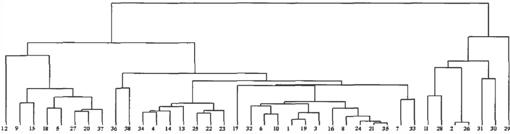
Now that a set of consistent CE answers is selected for each subject, we simultaneously start 38 random walks from 38 consistent utility functions, one for each sub­ ject. The radius f of the ball is initialized to 0.001. At each iterations, we g en era t e a random point in each ball of radius E. If the generated point is consistent with the constraints, we move to the new point and mark the iteration a success; otherwise we stay at the current location and call the iteration a failure. If two successes occur consecutively, we double the radius. If two failures occur consecutively, we halve the ra­ dius. We stop the random walk after 1000 iterations at which point we obtain a random sample of consis � tent utility functions for the 38 subjects. We compute the distance between any two consistent utility func­ tions and record the distances in a square dissimilarity matrix of size 38 x 38. This computation is performed by a routine that implements the algorithm in Table 1. We repeat the whole process for a total of 1000 times, updating the averages of the distances as we go. Fi­ nally, we input the average distance matrix to the hier­ archical clustering algorithm of ClustanGraphics ® to obtain the hierarchical clustering shown in Figure 1. The method used was average-linkage. 2

2 All of the codes were written in JavaTM and the math-

7 SUMMARY AND DISCUSSION

In previous work [8], we introduced the probabilis­ tic distance as a measure of dissimilarity among peo­ ple preferences, and provided algorithms to estimate this measure in the case of decision making under cer­ tainty. In this paper we complete the discussion of the probabilistic distance by providing algorithms to esti­ mate this measure in the uncertainty case. Under unc­ etainty, the problem is innately harder, because of the complexity introduced by probabilities and utilities. We have shown that with the reasonable assumption that the set of consistent utility functions is linearly bounded, computing the probabilistic distance can be reduced to the well-studied problem of computing the volumes of convex bodies for which efficient approxi­ mate algorithms exist. A key ingredient of these al­ gorithms is a Markov chain-based, polynomial time sampling algorithm that samples points from a con­ vex body according to a nearly uniform distribution. We use this sampling algorithm directly to estimate the probabilistic distance on partially specified utility functions. We demonstrate this procedure on a set of partially specified utility functions elicited from 44 subjects who are undergraduates at the University of Michigan. We show how the probabilistic distance be­ tween subjects can be computed based on arbitrary sets of answers to standard gamble questions. Note that in computing the probabilistic distance, we can incorporate any prior knowledge about user utilities in the form of utility constraints, as long as the con­ straints are linear. The more constraints there are, the more accurately the distance measure can be com­ puted. To our knowledge, this work is the first at­ tempt to define a similarity measure on partial utility functions and to develop a method to compute this measure. The implication of the probabilistic distance goes beyond the context of case-based preference elic­ itatio n , since it is in its most general form a distance measure on partial orders -a topic that has not been received adequate treatment.

We are currently investigating several medical decision problems as potential candidates for implementing the case-based preference elicitation approach. For such candidates, the basic requirement is that a database of patient utilities is available. Since utility data are routinely collected for a wide range of medical decision problems, and since the standard gamble CE method is one of the most widely used techniques to elicit util­ ities, we believe that the case-based approach using the probabilistic distance has serious potential to see

ematical programming language of MatLab®. The com­ putations were performed on an Athlon ™ @850Mhz sys­ tem with 512MB RAM running Windows® 2000, and took about an 30 minutes to finish.

二

1. M. D y er , A. Frieze, and R. Kannan. A random polynomial-time algorithm for a p p r o x im a t i ng the vol­ ume of convex b o d i e s . Journal of the ACM, 38(1) : 11 7, 1991.
2. R.E. Frank, W.F. M a ss y , and Y. W i n d . Market Seg­ mentation. Pr ent i ceH a l l , New Jersey, 1972.
3. V. H a and P. H ad d a wy . Towards case-based preference elicitation: Similarity measures on preference struc­ tures. In Proceedings of the Fourteenth Conference on Uncertainty in Artificial Intelligence, pages 193-201, July 1998.
4. V. Ha and P. Haddawy. A h yb r i d approach to reason­ ing with p a r tial p re fe rence models. In Proceedings of the Fifteenth Conference on Uncertainty in Artificial Intelligence, August 1999. To appear.
5. D. Kahneman and A. Tversky. Prospect theory: An analysis of of de c i si o n s under risk. Econometrica, 47:276-287, 1979.
6. [1 1] L. Lovasz, R. K a nn a n , and M. Simonovits. Random walks and an o * (n5) volume algorithm for convex b od i e s . Random Structures and Algorithms, 1 1 : 1-50, 1997.
7. J. M. Miyamoto and S. A. Eraker. Parametric models of the utility of survival: Tests of axioms in a ge n e r i c utility framework. Organizational Behavior and Hu­ man Decision Processes, 44:166-202, 1989.
8. [ 1 3] H. Nguyen and P. Haddawy. The decision-theoretic video advisor. In Proceedings of the 15th Conference in Uncertainty In Arti ficial Intelligence, 1999.
9. R. Pyke. Spacings. Journal of the Royal Statistical Society B, 27:395-436, 1965. Discussion: 437-49.
10. [ 15] P. Resnick, N. lacovou, M. Suchak, P. Bergstrom, and J. Reid!. Group lens: An open architecture for c ol ­ laborative filtering of n e tn ew s. In Proceedings of the 1994 Computer Supported Cooperative Work Confer­ ence, pages 175-186, New York, NY, 1994.
11. A. Tversky and D. Kahneman. Utility theory and additivity analysis of risky choices. Journal of Exp e r ­ imental Psychology, 75:27-36, 1967.
12. [ 1 7] J. von Neumann and 0. Morgenstern. Theory of Games and Economic Behavior. P ri nc e t o n Univesity Press, 1944.

real-world application.

Chajeswska et al. [3] pursue an approach to utility elicitation that is somewhat similar to ours. They also start from an assumption that there exists a database of utility functions, partially or completely specified. This assumption differs from ours in that here the database needs to contain the actual utilities ( as op­ posed to constraints on utilities ) . The novelty of this approach is that utilities are treated as random vari­ ables, and if drawn from a mixture of Gaussians, as they were postulated to, their density functions can be learned from the utility database using Bayesian learning techniques. Also, using standard Bayesian techniques, it is possible to determine the relevance of an elicitation question based on its value of informa­ tion [4] . In contrast, our case-based approach requires fewer structural assumptions and as such has an edge over Chajewska et al. 's approach in those situations where these assumptions are not applicable.

References

1. I. Barany and Z. Furedi. Computing the volume is difficult. In Proceedings of the 18th Annual Symposium on Theory of Computing, pages 442-447, May 1986.
2. R. Bubley and M. Dyer. Faster random generation of linear extensions. In Proceedings of the Ninth An­ nual A CM-SIAM Symposium on Discrete Algorithms, p age s 175-186, San Francisco, CA, Jan 1998.
3. U. Chajewska and D. Koller. U til i t i es as r a n d o m variables: Density estimation and s t r u c t u r e discov­ e r y. In Proceedings of the Sixteenth Conference on Un­ certainty in Artificial Intelligence, pages 63-71, July 2000.
4. U. Chajewska, D. K o l le r , and R. Parr. Making ratio­ nal decisions using adaptive util it y elicitation. In Proc AAAI 2000, pages 363-369, July 2000.
5. D. E. Critchlow. Metric Methods for Analyzing Par­ tially Ranked Data. Sp ri nger -Verlag, 1980. Lecture Notes in Statistics.