Soft Constraint Logic Programming for Electric Vehicle Travel Optimization /star

Giacoma Valentina Monreale 1 , Ugo Montanari 1 and Nicklas Hoch 2

1

Dipartimento di Informatica, Universit` a di Pisa, Italy

2 Volkswagen AG, Corporate Research Group Wolfsburg, Germany [email protected], [email protected] [email protected]

Abstract. Soft Constraint Logic Programming is a natural and flexible declarative programming formalism, which allows to model and solve real-life problems involving constraints of different types.

In this paper, after providing a slightly more general and elegant presentation of the framework, we show how we can apply it to the e-mobility problem of coordinating electric vehicles in order to overcome both energetic and temporal constraints and so to reduce their running cost. In particular, we focus on the journey optimization sub-problem, considering sequences of trips from a user's appointment to another one. Solutions provide the best alternatives in terms of time and energy consumption, including route sequences and possible charging events.

1 Introduction

Classical constraint satisfaction problems (CSPs) [12] represent an expressive and natural formalism useful to specify different types of real-life problems. A CSP can be described as a set of variables associated with a domain of values, and a set of constraints. A constraint is a limitation of the possible combinations of the values of some variables. So, solving a CSP consists in finding an assignment of values to all its variables guaranteeing that all constraints are satisfied.

Despite their applicability, the main limit suffered by CSPs is the ability of just stating if an assignment of certain values to the variables is allowed or not. This is indeed not enough to model scenarios where the knowledge is not either entirely available or not crisp. In these cases constraints are preferences and, when the problem is overconstrained, one would like to find a solution that is not so bad, i.e., the best solution according to the levels of preferences. For this reason, in [2,3], the soft CSP framework has been proposed. It extends classical constraints by adding to the usual notion of CSP the concept of a structure representing the levels of satisfiability or the costs of a constraint. Such a structure is represented by a semiring, that is, a set with two operations: one (usually denoted by +) is used to generate an ordering over the levels, while

/star Research partially supported by the EU FP7-ICT IP ASCEns .

the other one (denoted by × ) is used to define how two levels can be combined and which level is the result of such a combination.

Constraint logic programming (CLP) [10] extends logic programming (LP) by embedding constraints in it: term equalities is replaced with constraints and the basic operation of LP languages, the unification, is replaced by constraint handling in a constraint system. It therefore inherits the declarative approach of LP, according to which the programmer specifies what to compute while disregarding how to compute it, by also offering efficient constraint-solving algorithms.

However, only classical constraints can be handled in the CLP framework. So, in [4], it has been extended to also handle soft constraints. This has led to a highlevel and flexible declarative programming formalism, called Soft CLP (SCLP), allowing to easily model and solve real-life problems involving constraints of different types. Roughly speaking, SCLP programs are logic programs where constraints are represented by predicates which are defined by clauses whose body is a value of the semiring modelling the levels of satisfiability or the costs of the constraints. The flexibility of the approach is due to the fact that the same framework can be used to handle different kinds of soft constraints by simply choosing different semirings. It can indeed be used to handle fuzzy, probabilistic, prioritized and optimization problems, as well as classical constraints.

In this paper, before presenting an application of the SCLP framework to the e-mobility, we provide a slightly more general and elegant presentation of the SCSP framework based on the notion of named semiring, as briefly presented in [7]. In particular, soft constraints are elements of the named semiring which, besides the additive and multiplicative operations useful to combine the constraints, is equipped by a permutation algebra and a hiding operator allowing an explicit handling of names. The permutation algebra indeed allows to characterize the support of each constraint, that is, the subset of variables on which the constraint really depends, while the hiding operator allows us to remove variables from the support of a constraint. Then, the SCLP framework can be seen as the general case of the SCSP one.

We propose the SCLP framework as a high-level specification formalism useful to naturally model and also solve some e-mobility optimization problems. With e-mobility indeed new constraints must be considered: electric vehicles (EVs) have a limited range and they take long time to charge. So, it is needed to guarantee that throughout the user's itinerary the EV never underruns a limit energy level and that the user always arrives in time to all his appointments.

We consider the EV travel optimization problem described in [9]. In it the user has a set of appointments and he makes a series of decisions about the sequences of trips from an appointment to another one, for example which route to take, if and where to charge the EV and so on. The aim is to find the optimal combination of travel choices which minimizes the users cost criteria. In [9], the authors propose a hierarchical presentation of the mobility framework, which they exploit to decompose the optimization problem in sub-problems, and in particular, they study the journey level one. Here, beside it, we consider the optimization problem of the lower level, i.e., the one of the trip level. This last problem consists in finding the best trips in terms of travel time and energy consumption, while the former one consists in finding the optimal journey, that is, the optimal sequence of coupled trips, again in terms of the same criteria, guaranteeing that the user reaches each appointment in time and that the state of charge (SoC) of the EV never falls below a given threshold.

The trip level problem substantially coincides with the multicriteria version of the shortest path problem modelled in [5] as an SCLP program. So, starting from a slightly different specification of this problem, we propose an SCLP program modelling the journey problem. In order to also actually execute both the SCLP programs, we propose CIAO Prolog [6], a system supporting constraint logic programming. We therefore explicitly implement the soft framework, by defining two predicates, the plus and the times ones, which respectively model the additive and the multiplicative operations of the semiring.

This work arises from the research activity in the European project ASCENS (Autonomic Service Component ENSembles) aiming at studying formal models, languages, and programming tools, for the modelling and the development of autonomous, self-aware adaptive systems. E-mobility is right one of the case studies of the project and our work represents a first answer to the need of a high-level, declarative, executable specification language and of a powerful and flexible programming environment where e-mobility problems can be easily and naturally modelled and solved. We indeed show as the SCLP framework is able to satisfy all these requirements and it can thus be used as a support for rapid prototyping and exploratory programming for this kind of problems.

The paper is organized as follows. Section 2 introduces the SCSP framework as an instantiation of the named semiring framework. Section 3 briefly recalls the SCLP language and then Section 4 shows how the trip and journey optimization problems can be modelled and solved through (S)CLP programs. Finally, Section 5 concludes the paper by illustrating some open venues for further works.

2 Soft Constraints by means of Named Semirings

This section presents the soft CSP framework based on semiring [2,3] as an instantiation of the more general framework based on named semiring [7].

The notion of named semiring is based on the ones of c-semiring (c stands for constraint) and permutation algebra.

2.1 C-Semiring

Definition 1 (c-semiring). A c-semiring is a tuple 〈 A, + , × , 0 , 1 〉 such that:

• -A is a set and 0 , 1 ∈ A ;
• -+ : A × A → A is a commutative, associative and idempotent operation, such that 0 is its unit element and 1 is its absorbing element;
• -× : A × A → A is a commutative and associative operation, such that it distributes over + , 1 is its unit element, and 0 is its absorbing element.

Thanks to the idempotence of the + operator, the relation 〈 A, ≤〉 , defined as a ≤ b if a + b = b , is a partial order. Intuitively, a ≤ b means that b is better than a or that a implies b .

It is possible to prove that: (i) the two operations + and × are monotone on ≤ ; (ii) 0 is its minimum and 1 its maximum; (iii) 〈 A, ≤〉 is a complete lattice and + is its least upper bound 3 . Finally, if × is idempotent then: (iv)+ distribute over × ; (v) 〈 A, ≤〉 is a distributive lattice, and (vi) × is its greatest lower bound.

2.2 Permutation Algebra

Here we briefly recall the notion of permutation algebra . We refer the reader to [8] for a detailed introduction.

In the following, we fix a chosen infinite, countable, totally ordered set N of names, which we denote by x, y, z, . . . .

Definition 2 (Permutations). A name substitution is a function σ : N → N , while a permutation ρ is a bijective name substitution. The set of all such permutations on N is denoted by P ( N ) .

Definition 3 (Kernel). Let ρ ∈ P ( N ) be a permutation on N . The kernel of ρ is the set of the names that are changed by the permutation, formally, K ( ρ ) = { x ∈ N| ρ ( x ) = x } .

/negationslash

A permutation ρ is finite if its kernel is finite.

From now on we consider only finite permutations.

In the following, we introduce the notion of permutation algebra. It consists of a pair composed of a carrier set and a description of how the elements of the carrier set are transformed by permutations.

Definition 4 (Permutation Algebras). The permutation signature Σ p on N is defined as the set of unary operators { ̂ ρ | ρ ∈ P ( N ) } plus the two axioms ̂ id ( a ) = a and ̂ ρ 1 ( ̂ ρ 2 ( a )) = ̂ ρ 1 ρ 2 ( a ) .

A permutation algebra A = ( A, { ̂ ρ A } ) consists of a carrier set A and the set of the interpreted operations ̂ ρ A .

Definition 5 (Support). Let A be a permutation algebra and a an element of its carrier set. The support of a , supp ( a ) , is the smallest set of names such that, given a permutation ρ , if ρ ( x ) = x for all x ∈ supp ( a ) , then ̂ ρ A ( a ) = a .

Intuitively, supp ( a ) represents the free names of a : indeed the permutations which do not modify them are not influent on a .

Definition 6 (Finitely supported algebra). A permutation algebra A is finitely-supported if each element of its carrier has finite support.

3 Actually, in order to prove this result, we must assume that the sum of an infinite number of elements exists.

2.3 Named c-Semiring.

A named semiring [7] is a c-semiring plus a finitely-supported permutation algebra A and a hiding operator ( νx. ). The permutation algebra allows characterizing the finite set of free names of each element c of the named semiring (represented by the support of c ), while ( νx. ) applied to c makes the name x local in c .

Definition 7 (Fusion). A (name) fusion is a total equivalence relation on N with only finitely many non-singular equivalence classes. We denote by x = y the fusion with a unique non-singular equivalence class consisting of x and y .

Definition 8 (Named c-semiring). A named c-semiring C = 〈 C, + , × , νx., { ̂ ρ C } , 0 , 1 〉 is a tuple where: -x = y ∈ C for x, y ∈ N ; -〈 C, + , × , 0 , 1 〉 is a c-semiring; -〈 C, { ̂ ρ C }〉 is a finite-support permutation algebra; -νx. : C → C , for each name x , is a unary operation; -for all c, d ∈ C and for all ρ the following axioms hold: (FUSE) x = y × c iff x = y × [ y/x ] c (HIDE) νx. 1 = 1 νx.νy.c = νy.νx.c νx. ( c × d ) = c × νx.d if x /negationslash∈ supp ( c ) νx. ( c + d ) = c + νx.d if x /negationslash∈ supp ( c ) νx.c = νy. [ y/x ] c if y /negationslash∈ supp ( c ) (PERM) ̂ ρ C 0 = 0 ̂ ρ C 1 = 1 ̂ ρ C ( c × d ) = ̂ ρ C c × ̂ ρ C d ̂ ρ C ( c + d ) = ̂ ρ C c + ̂ ρ C d ̂ ρ C ( νx.c ) = νx. ( ̂ ρ C c ) if x /negationslash∈ K ( ρ )

In the (FUSE) axiom, [ y/x ] c denotes c where y is replaced by x .

2.4 The Named SCSP Framework

As briefly shown in [7], named c-semirings can be suitably instantiated to model SCSPs.

Definition 9 (Constraints). Let S = 〈 A, + , × , 0 , 1 〉 be a c-semiring, N a set of totally ordered names, and D a finite domain of interpretation for N . A soft constraint is a function ( N → D ) → A , which associates a value of A to each assignment η : N → D of the names.

We define C as the set of all soft constraints over N , D and A .

Definition 10. Let S = 〈 A, + , × , 0 , 1 〉 be a c-semiring, N a set of totally ordered names, and D a finite domain of interpretation for N . Moreover, let C be the set of all soft constraints over N , D and A . We define the C SCSP as the named c-semiring 〈C , + ′ , ⊗ , νx., { ̂ ρ C } , 0 ′ , 1 ′ 〉 , where fusions x = y are defined as ( x = y ) η = 1 if η ( x ) = η ( y ) and ( x = y ) η = 0 otherwise; ( c 1 + ′ c 2 ) η = c 1 η + c 2 η ; ( c 1 ⊗ c 2 ) η = c 1 η × c 2 η ; ( νx.c ) η = ∑ d ∈ D ( cη [ d/x ]) ; ( ̂ ρ C c ) η = cη ′ with η ′ ( x ) = η ( ρ ( x )) ; 0 ′ η = 0 and 1 ′ η = 1 ′ for all η .

The assignment η [ d/x ] is defined as usual: η [ d/x ]( y ) = d if x = y and η [ d/x ]( y ) = η ( y ) otherwise.

Note that, by definition, each constraint c ∈ C involves all the names in N , but it really depends on the assignment of the names in supp ( c ), and intuitively, restricting means eliminating a name from the support of the constraint, by choosing the best value for it.

Definition 11 (Soft CSP). A soft constraint satisfaction problem (SCSP) is a pair 〈 C, Y 〉 , where C ⊆ C is a set of constraints and Y ⊆ N is a set of names.

Intuitively, Y represents the set of interface names of the constraint set C .

Definition 12 (Solution). Let P = 〈 C, Y 〉 be an SCSP. The solution of P is the constraint Sol ( P ) = ( νx 1 ) . . . ( νx n )( ⊗ C ) , with { x 1 , . . . , x n } = ⋃ c i ∈ C supp ( c i ) \ Y .

Definition 13 (Best level). Let P = 〈 C, Y 〉 be an SCSP. Then, the best level of consistency of P is defined as the constraint blevel ( P ) = ( νx 1 ) . . . ( νx n )( ⊗ C ) , where { x 1 , . . . , x n } = ⋃ c i ∈ C supp ( c i ) .

Varying the semiring S , on which the named semiring C SCSP is based, several kinds of problems can be represented: we consider the semiring S CSP = 〈{ true, false } , ∨ , ∧ , f alse, true 〉 for classical CSPs; S FCSP = 〈{ x | x ∈ [0 , 1] } , max, min, 0 , 1 〉 for fuzzy CSPs; and S WCSP = 〈 N ∪{ + ∞} , min, + , + ∞ , 0 〉 for optimization CSPs.

Example 1. Let P be the SCSP with three names N = { x, y, z } , which can take values in D = { red, blue, green } . We assume that only x and y are of interest, while the constraints model the fact that all names must take different values.

We consider the semiring S WCSP , introduced above, and we define three constraints, one for each pair of names, c xy , c yz and c zx , associating the worst semiring value to the assignments which give the same color to both the names of interest for the constraint. In particular, we associate + ∞ to all the assignments giving the same color to both names, if at most one name takes the color red then we associate 1, otherwise we associate 2.

In Horn logic this problem can be expressed as the predicate P ( x, y ) below:

Q ( v, w ) : -if v = w then + ∞ else if either v or w are red then 1 else 2.

The predicate Q ( v, w ) represents the constraint shown on the left of Fig. 1, where the names v and w represents the only names of the support. Note that in this representation we only show the assignment for the names of the support of the constraint. Therefore, each table entry actually represents different entries, one for each possible color of the names which are not in the support. The constraint representing the problem is then represented by the combination of three constraints. Indeed, Q ( x, y ), Q ( y, z ) and Q ( z, x ) respectively represent the three constraints c xy , c yz and c zx , obtained by applying to the constraint represented by Q ( v, w ) the permutations mapping the names of the support v and w to the

Fig. 1. The constraint represented by Q ( v, w ) and the solution of the SCSP P .

x	y		v w
red red red blue blue blue green green green	red blue green blue red green green red blue	+ ∞ 1 1 + ∞ 1 2 + ∞ 1 2	red red red blue blue blue green green green	red blue green blue red green green red blue	+ ∞ 4 4 + ∞ 4 4 + ∞ 4 4
Q ( v,w )			Sol ( P )

names of interest of the three constraints. As said above, the relevant names of the problem are just x and y , thus the solution of the problem is obtained by combining the three constraints and restricting the scope of the name z . It can be expressed as ( νz )( c xy ⊗ c yz ⊗ c zx ). The resulting constraint, represented by the predicate P ( x, y ), is shown on the right of Fig. 1. Also in this case, we show the assignment of just the two names of the support. Each table entry is the minimum value among the ones of the solutions providing a different color for z . In this case, the best level of solution is 4, the minimum over all the entries.

3 Soft Constraint Logic Programming

This section briefly introduces the soft constraint logic programming (SCLP). For a more detailed and complete introduction, we refer the reader to [4].

The SCLP framework extends the classical constraint logic programming to also handle SCSPs. We can say that an SCLP program over a certain c-semiring S is just a CLP program where constraints are defined over S . In the following, we fix a semiring S = 〈 A, + , × , 0 , 1 〉 .

An SCLP program is hence a set of clauses composed of a head and a body, plus a goal. The head of a clause is simply an atom, while the body can be either a collection of atoms, or a c-semiring value, or a special symbol ✷ , denoting that it is empty. In this two last cases clauses are called facts and define predicates representing constraints. When the body is empty, we interpret it as 1, the best element of the semiring. Atoms are n -ary predicate symbols followed by a tuple of n terms, which can be either a constant or a variable or an n-ary function symbol followed by n terms. Ground terms are terms without variables, and finally, a goal is a collection of atoms.

Example 2. As an example, consider the simple SCLP program on the left of Fig. 2, previously proposed in [4]. We consider the semiring S KCSP and the domain D = { a, b, c } . The program is composed of six clauses. The last two are facts and the semiring values 2 and 3, associated respectively with the atoms

Fig. 2. An example of SCLP program and its fix point semantics.

			I 1	I 2	I 3	I 4
s(X)	:- p(X,Y).	t(a)	2	2	2	2
p(a,b)	:-	q(a). r(a)	3	3	3	3
		q(a)	+ ∞	2	2	2
p(a,c)	:-	r(a). p(a,c)	+	3	3	3
q(a)	:-	t(a).	∞
t(a)	:-	2. p(a,b)	+ ∞	+ ∞	2	2
	:-	3. s(a)	+ ∞	+ ∞	3	2
r(a)		s(b)	+ ∞ +	∞	+ ∞	+ ∞
		s(c)	+ ∞	+ ∞	+ ∞	+ ∞

t ( a ) and r ( a ), mean that they respectively cost 2 and 3 units. The set N of the semiring contains all possible costs, and the operations min and + allows us to minimize the sum of the costs. We consider as goal the atom :-s(a) : later on we will show its semantics.

Three equivalent semantics for the SCLP languages have been defined in [4]: the model-theoretic, the fix-point, and the operational one. These semantics are conservative extensions of the corresponding ones for logic programming: this means that by choosing the c-semiring S CSP we get exactly the LP semantics.

Actually, we can see the SCLP framework as the general case of the SCSP one. As shown in Example 1, we can indeed express an SCSP program as a set of predicates representing the constraints together with a unique clause which represents the problem and combines all constraints. In the case of the SCLP, the main difference is that the depth of clause nesting is unlimited and the possible values D of variables are elements of the Herbrand universe. So, the meaning of a predicate P ( x, y ) assigns a semiring value to all evaluations of variables x and y to the Herbrand domain. This is exactly what for example the fix-point semantics of the SCLP language does.

In order to present the fix-point semantics, we need to introduce the notion of interpretation and the T P operator, mapping interpretations into interpretations.

Definition 14 (Interpretation). An interpretation I consists of a domain D , representing the Herbrand universe, together with a function which takes a predicate and an instantiation of its arguments (that is, a ground atom), and returns an element of the semiring: I : ⋃ n ( P n → ( D n → A )) , where P n represents the set of n-ary predicates and A is the set of the values of the semiring.

Since interpretations are functions from ground atoms to semiring values, we consider programs composed of clauses where the head and the body contain only ground atoms. So, for example, in the SCLP program of Example 2, the clause s(X) :- p(X,Y) is replaced with all its instantiations. In particular, for each d ∈ D , we have three clauses s(d) :- p(d,a) , s(d) :- p(d,b) , and s(d) :- p(d,c) .

Definition 15 ( T P Operator). Let P be an SCLP program and IS P the set of all its interpretations. Moreover let I be an interpretation and GA a ground atom, such that P contains k clauses defining the predicate in GA and the clause i is of the shape GA : -B i 1 , . . . , B i n i . Then, we define the operator T P : IS P → IS P as T P ( I )( GA ) = ∑ k i =1 ( ∏ n i j =1 I ( B i j )) . Whenever B i j is a semiring value, its meaning I ( B i j ) is fixed in any interpretation I and it is the semiring value itself.

Definition 16 (Partial Order of Interpretations). Let P be a program and IS P the set of all its interpretations. We define the structure 〈 IS P , /precedesequal〉 , where ∀ I 1 , I 2 ∈ IS P , I 1 /precedesequal I 2 if I 1 ( GA ) ≤ I 2 ( GA ) for any ground atom GA , where ≤ is the order induced by the semiring.

Note that 〈 IS P , /precedesequal〉 is a complete partial order and its glb coincides with the glb operation in the lattice A (extended to interpretations). Since the function T P is monotone and continuous over this complete partial order, then T P has a least fix-point lfp ( T P ) = glb ( { I | T P ( I ) /precedesequal I } ) and it can be obtained by computing T P ↑ ω , i.e., by applying T P to the bottom of the partial order of interpretations, and then repeatedly applying it until a fix-point.

Example 3. Consider again the SCLP program in Fig. 2. In the definition of the T P operator we have to consider the additive and multiplicative operations of the semiring S KCSP , that is, the min and + operations. As in [4], we start the computing of the semantics from the bottom of the partial order of interpretations, I 0 , which maps each semiring element into itself and each ground atom into + ∞ . The table on the right of Fig. 2 shows the value associated by the interpretations to the most interesting ground atoms. The interpretation I 4 represents the fix-point of T P . As an example, we show the computation for one of the most interesting case, the ground atom s(a) , which also corresponds to our goal. We said that the clause s(X) :- p(X,Y) is considered equivalent to all its instantiations. Therefore, I 4 ( s ( a )) = min { I 3 ( p ( a, a )) , I 3 ( p ( a, b )) , I 3 ( p ( a, c )) } = min { + ∞ , 2 , 3 } = 2.

4 The Electric Vehicle Travel Optimization Problem

This section presents the EV travel optimization problem, introduced in [9], and shows how it can be naturally modelled and solved in the SCLP framework.

General description of the problem. A user has a set of appointments, each of them is in a location and has a starting time and a duration. The user makes a series of decisions regarding the sequences of trips from an appointment to another one. For example, he decides which route he wants to follow, where to park and if and how to charge the EV at the appointment location.

All possible combinations of travel choices form the choice set. A travel choice is optimal if it minimizes the users cost criteria.

In particular, finding a single optimal trip consists in finding the best trips in terms of travel time and energy consumption. Finding instead the optimal journey, that is, the optimal sequence of coupled trips, consists in finding the best journeys not only in terms of travel time and energy consumption, but also in terms of other important criteria for the user, such as the charging cost, the number of charging events, etc. However, in finding the solution it needs to guarantee that the user reaches each appointment in time and that the state of charge (SoC) of the vehicle never falls below a predefined threshold.

In [9], the authors propose a hierarchical presentation of the e-mobility framework, which they exploit to decompose the optimization problem in suboptimization problems. In particular, they identify four levels of mobility: the component level , whose main tasks are the inter- and intra-component coordination; the trip level , whose main task is the time and energy optimal routing; the journey level , which handles sequences of trips together with charging and parking strategies; and the mobility level , which handles mobility services, such as, car and ride service.

Each level represents a different optimization problem and the results of the lower level will be inputs of the higher level. However, since, in general, the best solution of the lower level could be not optimal for the higher one, the results of the lower level could contains several solutions and not only the best one.

In the following, we consider only the trip level and the journey level optimization problems. In particular, we first present their formalization and then we show how we can model them in the SCLP framework.

Formalizations of the trip and journey level optimization problems.

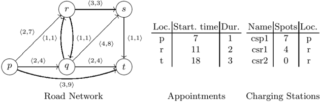
The trip level optimization problem substantially coincides with the multicriteria shortest path problem. The road network is indeed represented by a directed graph G := ( N,E ), where each arc e ∈ E from a node p to a node q has associated a label 〈 c T , c E 〉 , that is, a pair whose elements represent the costs, respectively in terms of time and energy consumption, of the arc from p to q .

So, given the road network G , such as the one on the left of Fig. 3, a source node n s and a destination node n d , the problem consists in finding all the best paths between n s and n d in terms of time and energy consumption. Note that, since the costs of the arcs are elements of a partially ordered set, the solution can contain several paths, that is, all paths which are not dominated by others, but which have different incomparable costs. For example, if we want to know the best paths from p to t in the graph of Fig. 3, the solution will contain both the paths { p, t } with cost 〈 3 , 9 〉 and { p, q, t } with cost 〈 4 , 8 〉 . The former is indeed better in terms of time while the latter in terms of energy consumption.

As far as the journey level optimization problem is concerned, we use the formalization presented in [9]. Actually, we consider a simpler version of it, which avoids to consider car parks and the time that the users would take to go from either the car park or the charging station to the location of the appointment. Moreover, we consider only the time and energy consumption as cost criteria to be minimized. All these simplifications allows a slender and more readable presentation of the SCLP program modelling the problem.

Let A = { A 1 , . . . , A n } be the set of the user's appointments. In order to describe the problem, we use different time variables. All of them have the shape i t Y Z , where i denotes the appointment, Y ∈ { D,A } ( D stands for drive and A for appointment), and Z ∈ { S, E } ( S stands for start and E for end).

/d47

/d53

/d53

/d47

/d47

/d47

Fig. 3. The road network, the user's appointments and the charging stations.

Each appointments is defined by a location L i , a starting time i t A S , an end time i t A E and therefore a duration i d A . In order to go from an appointment A i to the next one A i +1 , the user leaves with an EV from the location L i at time i t D S and drive to location L i +1 . The user travels along the route alternative iR D (computed by the trip level problem), which consumes energy and hence reduces the SoC. Obviously, the chosen route must allow the user to arrive to destination with the SoC of his EV. We assume that the SoC always decreases during driving and increases during charging events 4 . The user arrives at i t D E and the appointment starts at i t A S . The user must arrive in time to the appointment, so it is required that i t D E ≤ i t A S . During the appointment, it is also possible to schedule a charging event if the SoC of the EV is not enough to continue the journey. We assume to have a set of charging stations. Each of them is simply defined by its name CSname , the number of available charging spots SpotsNum , and the location L where it is.

Therefore, given the road network G , a set of appointments, as the ones described in the table in the middle of Fig. 3, and a set of charging stations, as the ones in the rightmost table of Fig. 3, the problem consists in finding all the best journeys through all the appointment locations in terms of time and energy consumption. As for the travel optimization problem, also here the solution can contain several journeys, that is, all the non-dominated ones.

SCLP programs for the optimization problems. In the following, we show how the SCLP framework can be used as a linguistic support and a high-level and flexible programming environment where naturally modeling and solving the two optimization problems presented above.

As far as the trip level optimization problem, we propose a slightly different version of the model proposed in [5] for the multi-criteria shortest path problem. So, as there, we consider an SCLP program over the c-semiring denoted P H ( S ) which, given a source node n s and a target node n d , allows us to obtain the set of the costs of all non-dominated paths from n s to n d .

4 This is the typical behaviour of EVs, however, as explained in [9], in particular cases it might also increase during driving and decreases during charging.

/d63

/d63

/d74

/d74

/d10

/d10

/d47

/d47

/d63

/d63

/d15

/d15

findall([P,T,E],path(X,Y,P,[X],[T,E],Lim),ResL),

:-module(paths,_,_). :-use_module(library(lists)). :-use_module(library(aggregates)). minPair([T,E],[T1,E1]):T < T1, E < E1. times([T1,E1],[T2,E2],[T3,E3]):T3 = T1 + T2, E3 = E1 + E2. plus([],L,[]). plus([[P,T,E]|RestL],L, [[P,T,E]|BestPaths]):nondominated([T,E],L), plus(RestL,L,BestPaths). plus([[P,T,E]|RestL],L,BestPaths):\+nondominated([T,E],L), plus(RestL,L,BestPaths). nondominated([T,E],[]). nondominated([T,E],[[P,T1,E1]|L]):\+minPair([T1,E1],[T,E]), edge(p,q,[2,4]). edge(q,t,[2,4]). edge(p,r,[2,7]). edge(r,s,[3,3]). edge(p,t,[3,9]). edge(r,q,[1,1]). edge(q,r,[1,1]). edge(s,t,[1,1]). edge(q,s,[4,8]). path(X,Y,[X,Y],_,[T,E],Lim):edge(X,Y,[T,E]), E =< Lim. path(X,Y,[X|L],V,[T,E],Lim):edge(X,Z,[T1,E1]), nocontainsx(V,Z), path(Z,Y,L,[Z|V],[T2,E2],Lim), times([T1,E1],[T2,E2],[T,E]), E =< Lim. paths(X,Y,Lim,BestPaths):plus(ResL,ResL,BestPaths).

nondominated([T,E],L).

The semiring P H ( S ) is obtained starting from a semiring S = 〈 A, + , × , 0 , 1 〉 , which in our case is the one modelling the costs associated to each edge, i.e, S = 〈 N 2 , min ′ , + ′ , 〈∞ , ∞〉 , 〈 0 , 0 〉〉 , where min ′ and + ′ are the min and + operations extended to pairs. Indeed, in general we want to minimize the sum of each cost, but, since we want to obtain all the non dominated paths, we consider P H ( S ).

Given a semiring S , we define P H ( S ) = 〈 P H ( A ) , /unionmulti , × ∗ , ∅ , A 〉 , where P H ( A ) is the Hoare Power Domain of A , that is, P H ( A ) = { S ⊆ A | x ∈ S, y ≤ S x implies y ∈ S } . These sets are isomorphic to those containing just the nondominated values, thus, in the following, we will use this more compact and efficient representation, where each element of P H ( A ) will represent the costs of all non-dominated paths from a node to another one. The top element of the semiring is the set A (its compact form is { 1 } , which in our example is {〈 0 , 0 〉} ); the bottom element is the empty set; /unionmulti is the formal union that takes two sets and gives their union; × ∗ takes two sets and produces another one obtained by multiplying (using the multiplicative operation of the original semiring, in our case + ′ ) each element of the first set with each element of the second one.

Note that, in the partial order induced by the additive operation of this semiring, a ≤ P H ( S ) b intuitively means that for each element of a , there exists an element of b which dominates it (in the partial order of the original semiring).

Following [5], in order to also really execute the SCLP program, we model the problem with a program in CIAO Prolog [6], a system supporting CLP, by explicitly implementing the soft framework. The program is shown in Fig. 4.

Here we consider the road network presented in Fig. 3, so we have a set of clauses modelling it. In particular, we have a set of facts modelling all the edges

Ciao 1.14.2-13646: Mon Aug 15 10:49:59 2011 ?-paths(p,t,10,BestPaths). BestPaths = [[[p,t],3,9],[[p,q,t],2+2,4+4]] ?. no ?-

of the graph. Each fact has the shape edge ( n s , n d , [ c T , c E ]), where n s represents the source node, n d represents the destination node and the pair [ c T , c E ] represents the costs of the edge in term of time and energy. Note that, differently from what would happen in the pure SCLP framework, these facts (representing constraints) have the cost in the head of the clauses and not in the body. This is needed for implementing the soft framework, and in particular the two operations of the semiring.

Moreover, there are two clauses path describing the structure of paths: the upper one models the base case, where a path is simply an edge, while the lower one represents the recursive case, where a path is an edge plus another path. The head of the path clauses has the following shape path ( n s , n d , L N , L V , [ c T , c E ] , Lim ), where n s and n d are respectively the source and destination nodes, L N is the list needed to remember, at the end, all the visited nodes of the path in the ordering of the visit, L V is the list of the already visited nodes needed to avoid infinite recursion where there are graph loops, [ c T , c E ] is used to remember the cost of the path in terms of time and energy, and finally, Lim represents the maximum amount of energy that the EV can consume. It is used to retrieve only the paths with a total cost in terms of energy equal to or less than the passed value.

The times and plus clauses are useful to model the soft framework. In particular, the first clause is useful to model the multiplicative operation of the semiring allowing us to compose the global costs of the edges together, time with time and energy with energy. The plus predicate instead mimics the additive operation and it is useful to find the best, i.e. non-dominated, paths among all the possible solutions. The plus predicate is indeed used in the body of the paths clause, which collects all the paths from a given source node to a given destination node and returns the best solutions chosen with the help of the plus predicate. So, if we want to know the best paths, in the graph of Fig. 3, from p to t with a total cost in terms of energy consumption less than or equal to 10, we have to perform the CIAO query paths ( p, t, 10 , BestPaths ), where the BestPaths variable will be instantiated with the list containing all the nondominated paths. In particular, for each of them, the list will contain the sequence of the nodes in the path and the total cost of the path in terms of time and energy. The output of the CIAO program for this query is shown in Fig. 5.

Now, by using the SCLP program modelling the travel optimization problem, we can also show the one modelling the journey level problem. Also in this case, as before, we consider the P H ( S ) semiring and we propose a CIAO program, where we also model the soft framework. The CIAO program modelling the journey optimization problem is presented in Fig. 6.

:-module(journey,_,_). :-use_module(paths). plus([],L,[]). plus([[P,T,E,ChEv]|RestL],L, [[P,T,E,ChEv]|BestPaths]):nondominated([P,T,E],L), plus(RestL,L,BestPaths). plus([[P,T,E,ChEv]|RestL],L, BestPaths):\+nondominated([P,T,E],L), plus(RestL,L,BestPaths). nondominated([P,T,E],[]). nondominated([P,T,E], [[P1,T1,E1,ChEv1]|L]):\+minPair([T1,E1],[T,E]), nondominated([P,T,E], L). appointment(p,7,1). appointment(r,11,2). appointment(t,18,3). chargingStation(csp1,7,p). chargingStation(csr1,4,r). chargingStation(csr2,0,r). journeys(Places,EV,BestJourneies):findall([P,T,E,ChEv],journey(Places,P,ChEv,[T,E],SoC),ResL), plus(ResL,ResL,BestJourneies). journey([X,Y],[P],[],[T,E],SoC):appointment(X,Tx,Dx), appointment(Y,Ty,Dy), path(X,Y,P,[X],[T,E],SoC), timeSum(Tx,Dx,T,ArrT), ArrT=

We have a set of facts modelling the user's appointments and the charging stations. In particular, for each appointment A i , there is a clause appointment ( L i , i t A S , id A ), while for each charging station we have a clause chargingStation ( CSname,SpotsNum,L ) .

Moreover, there are four journey clauses describing the structure of journeys. The upper two represent the base case, while the other two represent the recursive case. The first clause models the case where a journey is simply a path with a cost in terms of energy less than or equal to the SoC of the EV. The second clause models the case where the SoC of the EV is not enough to do any path and so a charging event, incrementing the energy level, must be scheduled. The third journey clause represents the case where a journey is a path with a cost in terms of energy less than or equal to the SoC of the EV, plus another journey. Finally, the last clause models the recursive case where a charging event is needed. In all cases we check that the paths allow the user to arrive in time.

The head of the journey clauses has the shape journey ( L L , L P , L ChEv , [ C T , C E ] , SoC ), where L L is the list of the locations of the appointments, L P is the list needed to remember, at the end, all the paths of the journey in the correct ordering, L ChEv is the list needed to

Ciao 1.14.2-13646: Mon Aug 15 10:49:59 2011 ?-journeys([p,r,t],10,BestJourneys). BestJourneys = [ [[[p,r],[r,s,t]],2+(3+1),7+(3+1),[[r,csr1]]], [[[p,r],[r,q,t]],2+(1+2),7+(1+4),[[r,csr1]]], [[[p,q,r],[r,s,t]],2+1+(3+1),4+1+(3+1),[]], [[[p,q,r],[r,q,t]],2+1+(1+2),4+1+(1+4),[]] ] ?. no ?-

remember all the charging events needed to complete the journey, [ C T , C E ] represents the cost of the journey in terms of time and energy, and finally, SoC represents the current energy level of the EV.

To make the program as readable as possible, we omit the predicates newSoC and timeSum , useful to respectively compute the new energy level of the EV after a charging event and the arriving time of the user to an appointment.

The plus clauses are useful to model the soft framework and they are very similar to the ones of the trip level problem. The only difference is that here we have to consider the charging events. Moreover, note that we reuse the times predicate defined in the CIAO program in Fig. 4.

The journeys clause collects all the journeys through a set of locations (the ones of the user's appointments) and returns the best solutions chosen with the help of the plus predicate. So, if we want to know the best journeys, in the graph of Fig. 3, through the locations where the user has the appointments, with an EV having an energy level equal to 10, we have to perform the CIAO Prolog query journeys ([ p, r, t ] , 10 , BestJourneys ), where p, r, t are the locations of the appointments and the BestJourneys variable will be instantiated with the list containing all the non-dominated journeys. In particular, for each of them, the list will contain the sequence of the paths of the journey, the total cost of the journey in terms of time and energy, and the list of the charging events, each of them described by the name of the charging station and its location. The output of the CIAO program for this query is shown in Fig. 7.

5 Conclusion

In this paper we proposed the SCLP framework as a high-level declarative, executable specification notation to model in a natural way some aspects of the e-mobility optimization problem [9], consisting in coordinating electric vehicles in order to overcome both energetic and temporal constraints. In particular, we considered the trip and journey optimization sub-problems, consisting in finding respectively the energyand time-optimal route from one destination to another one, and the optimal sequence of coupled trips, in terms of the same criteria, guaranteeing that the user reaches each appointment in time. For both the optimization problems, we provided an SCLP program in CIAO Prolog, by explicitly implementing the soft framework, that is, the additive and the multiplicative operations of the chosen semiring. The former is a slight variant of the CIAO program proposed in [5, Section 4.4] to specify the multicriteria version of the shortest path problem. With respect to the program proposed there, here we implemented a different semiring, (also proposed in [5]), i.e., the one based on the Hoare Power Domain operator, which allowed us to obtain only the best (i.e. non-dominated) routes in terms of time and energy consumption. We thus provided an implementation of the two operations of this semiring, by defining two predicates modelling them. The SCLP program modelling the journey optimization problem then uses the trip optimization problem results as inputs. It is also based on the same semiring that, in this case, allowed us to find the best journeys in terms of the two cost criteria.

As said above, the soft framework is explicitly implemented into each CIAO program: there is for example a different plus predicate in each optimization program we have proposed. However, it would be interesting to study a general way to embed the soft framework in Ciao Prolog. Trivially, one could provide a library offering a more general implementation of the operations of the semiring of each type of problem. Most interestingly, one could instead think to provide a meta-level implementing more efficiently the soft framework.

Differently from our solution, which allows us to obtain the set of all the optimal journeys, in the mathematical model proposed in [9] a form of approximation is introduced, by considering an aggregated cost function to be optimized. Their goal is indeed to minimize this cost function, which considers different cost criteria: besides the travel time and the consumed energy, they also take into account the charging cost, the number of charging events, etc. In modelling the problem, here we introduced a simplification by considering just the two main cost criteria, that allows us a slender presentation of the work. However, it is obvious that the SCLP programs can be easily modified to also take into account several other cost criteria. On the other side, we preferred not to introduce any approximation of the solution, by instead returning all optimal journeys considered equivalently feasible. However, since the use of partially ordered structures, as in our case, can in general lead to a potentially exponential number of undominated solutions, sometimes it becomes crucial to keep the number of configurations as low as possible through some form of approximation allowing us to adopt a total order. In this case, the right solution could be to adopt a function that composes all the criteria in a single one and then to choose the best tuple of costs according to the total ordering that the function induces [5, Section 6.1].

As said above, our aim is mainly to propose the SCLP framework as an expressive and natural specification language to model optimization problems. We indeed think that not only problems representing an extension of the one treated here can be modelled by adapting the solution we presented easily enough, but that in general our approach can be followed to model hierarchical optimization problems. All the SCLP programs we proposed are effective only when data of small size are considered. We are indeed conscious that the proposed encodings cannot be used to really solve the problem on practical cases, but on the other side, we think that CIAO represents a powerful system programming environment allowing us not only to write declarative specifications but also to reason about them.

It is therefore clear that here we do not take care of the performances of the proposed programs and that our aim is not to compare the performance with existing algorithms solving these problems. We indeed leave as future work the study of how to improve the performance of our programs. In [5, Section 8], the authors show some possible solutions that could be used towards this end, such as tabling and branch-and-bound techniques (implementable for example in ECLiPSe [1]). We however would also like to study how our programs can take advantage of the use of dynamic programming techniques based, for example, on the perfect relaxation algorithm for CSPs [11].

Finally, from a theoretical point of view, as future work, we plan to propose a more general framework based on named semiring, allowing us to give a unifying presentation of the SCSP and SCLP frameworks, providing an explicit handling of the names.

References

1. Apt, K.R., Wallace, M.: Constraint logic programming using Eclipse. Cambridge University Press (2007)
2. Bistarelli, S., Montanari, U., Rossi, F.: Constraint solving over semirings. In: IJCAI (1). pp. 624-630 (1995)
3. Bistarelli, S., Montanari, U., Rossi, F.: Semiring-based constraint satisfaction and optimization. J. ACM 44(2), 201-236 (1997)
4. Bistarelli, S., Montanari, U., Rossi, F.: Semiring-based contstraint logic programming: syntax and semantics. ACM TOPLAS 23(1), 1-29 (2001)
5. Bistarelli, S., Montanari, U., Rossi, F., Santini, F.: Unicast and multicast QoS routing with soft-constraint logic programming. ACM TOCL 12(1), 5 (2010)
6. Bueno, F., Cabeza, D., Carro, M., Hermenegildo, M., L´ opez-Garc´ ıa, P., Puebla, G.: The ciao prolog system. Reference manual. Tech. Rep. CLIP3/97.1, School of Computer Science, Technical University of Madrid (UPM) (1997)
7. Buscemi, M., Montanari, U.: Cc-pi: A constraint-based language for specifying service level agreements. In: ESOP. LNCS, vol. 4421, pp. 18-32. Springer (2007)
8. Gadducci, F., Miculan, M., Montanari, U.: About permutation algebras, (pre)sheaves and named sets. HOSC 19(2-3), 283-304 (2006)
9. Hoch, N., Zemmer, K., Werther, B., Siegwarty, R.Y.: Electric vehicle travel optimization - customer satisfaction despite resource constraints. In: IEEE IVS (2012)
10. Jaffar, J., Lassez, J.L.: Constraint logic programming. In: POPL. pp. 111-119. ACM Press (1987)
11. Montanari, U., Rossi, F.: Perfect relaxation in constraint logic programming. In: ICLP. pp. 223-237 (1991)
12. Tsang, E.: Foundations of constraint satisfaction. Computation in cognitive science, Academic Press (1993)