二

Solving Influence Diagrams using HUG IN, Shafer-Shenoy and Lazy Propagation

Anders L. Hugin Expert NS Niels Jernes Vej 10

DK-9220 Aalborg 0, Anders.L.Madsen@ hugin.com

Madsen Box 8201 Denmark

Abstract

In this paper we present three different architec­ tures for the evaluation of influence diagrams: HUGIN, Shafer-Shenoy (S-S), and Lazy Prop­ agation (LP). HUGIN and LP are two new ar­ chitectures introduced in this paper. The compu­ tational complexity using the three architectures are compared on the same structure, the Limited Memory Influence Diagram (LIMID), where on­ ly the requisite information for the computation of optimal policies is depicted. Because the req­ uisite information is explicitly represented in the diagram, the evaluation procedure can take ad­ vantage of it. Previously, it has been shown that significant savings in computational time can be obtained by performing the calculation on the LIMID rather than on the traditional influence diagram. In this paper we show how the ob­ tained savings is considerably increased when the computations are performed according to the LP scheme.

1 Introduction

In the last decade, several architectures have been proposed for the evaluation of influence diagrams. The pioneering ar­ chitecture was proposed by Olmsted (1983), and Shachter (1986). Their method works directly on the influence di­ agram by eliminating the nodes from the diagram in a re­ verse time ordering. Shenoy (1992) proposed an alterna­ tive formulation, valuation based systems, for the repre­ sentation and evaluation of such decision problems. Later on, Jensen et al. (1994) described an algorithm that solves influence diagrams by the propagation of messages in so­ called strong junction trees.

Recently, Lauritzen and Nilsson (1999) introduced the no­ tion of Limited Memory Influence Diagrams (LIMIDs) to describe multistage decision problems, and presented a

Dennis Nilsson

Department of Mathematical Sciences Aalborg University Fredrik Bajers Vej 70 DK-9220 Aalborg 0, Denmark nils son @math.auc.dk procedure, termed Single Policy Updating (SPU), for eval­ uating them. In contrast with traditional influence dia­ grams, LIMIDs allow for the possibility of violating the 'no-forgetting' assumption. Thus, in particular any influ­ ence diagram can be represented as a LIMID whereas the converse does not hold in general. In Nilsson and Lau­ ritzen (2000), it is shown how SPU applied on influence diagrams, can yield significant savings in computational time when compared to traditional influence diagram al­ gorithms. In the above paper, the computations performed during SPU were done by the passage of messages in a suit­ able junction tree using the S-S architecture.

In this paper we show how SPU for influence diagrams can be performed using two new architectures: The LP ar­ chitecture which has some resemblance with the method described in Madsen (1999), and the Hugin architecture which has some resemblance with the method described in Jensen et al. (1994). A comparison of the computational efficiency of the three architectures is then presented.

2 LIMIDs

A LIMID is a directed acyclic graph consisting of three types of nodes: Chance nodes representing random vari­ ables, decision nodes representing decisions to be taken, and value nodes representing (local) utility functions. The three types of nodes are represented as circles, boxes, and diamonds, respectively. The set of chance nodes is denoted r. the set of decision nodes is denoted by�. and the set of value nodes is denoted by Y.

The arcs in the LIMID have a different meaning depend­ ing on their destination. Arcs into chance nodes represent probabilistic dependence, and associated with chance node r is a conditional probability function Pr of the variable given its parents. Arcs into decision nodes are informa­ tional, and the parents of decision node d are the variables whose values are known to the decision maker at the time the decision d must be taken. Arcs into value nodes indi­ cate functional dependence, and the parents of value node u are the variables that the local utility function Uu. associ-

ated with u depends on.

In contrast with traditional influence diagrams, the infor­ mational arcs in LIMIDs are not restricted to obey the 'no­ forgetting' assumption. This assumption states that an ob­ servation made prior to a given decision must be known to the decision maker on all subsequent decisions. Since no-forgetting is not assumed in LIMIDs, the LIMID evalu­ ation algorithm (SPU) can take advantage of this flexibility, by removing informational arcs into decision nodes that are not neccessary for the computation of the optimal strategy. The removal of informational arcs are determined solely from the structure of the LIMID, and is performed prior to any numerical evaluation of the LIMID.

2.1 Strategies

We let V = r U .6.. Elements in V will be termed variables or nodes interchangeably. The variable n E V can take val­ ues in a finite set Xn. For W � V, we let Xw == XnewXn. Elements of Xw are denoted by lower case letters such as xw, abbreviating xv to x. The set of parents of a node n is denoted pa(n). The f amily of n, denoted fa(n), is defined by fa( n) = pa( n) U { n } .

A policy for decision node d is a function dd that as­ sociates with each state Xpa(d) a probability distributi � n 8d(-i Xpa(d)) on Xd. A uniform policy ford, denoted 8d, is given by Jd = 1/IXdl· A strategy q is a collection of policies q = {8d : d E .6.}, one for each decision. The strategy q induces a joint distribution of all the variables in Vas

The expected utility of a strategy q is the expectation of the total utility U = LuEY Uu wrt. the joint distribution of V induced by q: EU(q) = Lx /q(x)U(x). A global maximum strategy, or simply an optimal strategy, denot­ ed q, is a strategy that maximizes the expected utility, i.e. EU ( q ) ? EU ( q ) for all strategies q. The individual poli­ cies in an optimal strategy are termed optimal.

2.2 Single Policy Updating

SPU is an iterative procedure for evaluating general LIM­ IDs. The procedure starts with an initial strategy and im­ proves it by local updates until convergence has occurred, i.e. until every local change would result in an inferior stra­ tegy. Given a strategy q = { 8d : d E .6.} and do E 6, we let Q-do = q \ { 6do} be the partially specified strategy ob­ tained by retracting the policy for do from q.

SPU starts with an initial strategy and proceeds by modi­ fying (updating) the policies in a random or systematically order. If the current strategy is q and the policy for d; is to be updated, then the following steps are performed:

• Retract: Retract the current policy for d; from q to obtain Q-d;.
• Optimize: Compute a new policy ford; by:

• Replace: Redefine q :== Q-d; U {Jd.}.

The policies are updated until they converge to a strategy in which no single policy modification can increase the ex­ pected utility.

2.3 Single Policy Updating for Influence Diagrams

Suppose we apply SPU on a traditional influence diagram with decision nodes 6 = { d1, . · . , dk}, where the index of the decisions indicate the order in which they are to be tak­ en, i.e. d1 is the initial decision, and dk is the last decision to be taken. In this case, we always compute an optimal strategy using SPU, if we

• start with the uniform policies on all the decisions;
• update the policies for the decisions using the order dk, . . . , d l.

Furthermore, the optimal strategy is computed after exactly one update of each policy.

When the policy for di is to be updated, the optimal policy for di is found by computing (letting d = di)

where o;. are optimal policies for dj. j = i + 1, .. . ' k. '

Note that in the expression (2), the uniform policies for d1, . . . , di-l are not included. This is because they have no effect on the maximizing policy od, .

2.4 Construction of the junction tree

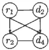
SPU is performed efficiently in a computational structure called junction tree. We abstain here from explaining all the details in the compilation procedure, but refer to Lau­ ritzen and Nilsson (1999) for further reading. In brevity, the compilation of a LIMID into a junction tree consists of four steps, see Fig. I :

Reduction: Here, all non-requiste informational arcs i n to the decision nodes are removed. A non-requiste arc from a node n into decision node d has the property that there exists an optimal policy for d that does not depend on n. Denote the obtained LIMID Lmin·

Moralization: In this step, pair of parents of any node in Lmin are 'married' by inserting a link between them. Then, the diagram is made undirected, and finally util­ ity nodes are removed. Denote the obtained undirect­ ed graph by em.

Triangulation: Here em is triangulated to obtain

£1.

Construction of the junction tree: In this final step, a junction tree is constructed whose nodes correspond to the cliques of ct .

In the Triangulation step it is important to note that any tri­ angulation order may be used. As a nice consequence, our junction tree is typically smaller than the strong junction tree as described in Jensen et al. (1994).

2.5 Partial collect propagation

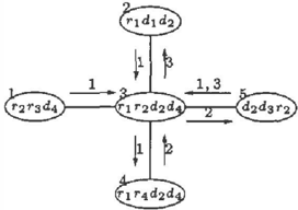
Suppose we are given the junction tree representation T of a LIMID C with decision nodes d1, ... , dk. Initially, we update the policy for the last decision dk by passing messages from the leaves ofT towards any one clique con­ taining fa(dk)· After this 'collect operation', a local opti­ mization is performed to compute the updated policy for dk. The local optimization processes differ slightly for the three architectures and are explained later. Next, the policy for decision dk-l is updated, and we could apply the same algorithm for this purpose. This procedure suggests that we have to perform k collect operations in the course of the evaluation of the LIMID. The procedure usually involves a great deal of duplication. After the first collect operation towards any clique, say Rk, containing fa(dk), we must collect messages towards any one clique, say Rk-t, con­ taining fa( dk-d. However, because some of the messages have already been performed during the first collect opera­ tion, we need only pass messages from Rk towards Rk-l· Thus, it can be seen that we need only perform one 'full' collect (towards Rk), and k -1 'partial' collect operations, see Fig. 2 for an illustration of the partial collect algorithm.

3 The Shafer-Shenoy architecture

In our local propagation scheme, the utilities and probabil­ ities specified in the LIMID £ are represented by entities called potentials:

Definition 1 [Potential]

A potential on W � V is a pair 1rw = (pw, u w) where Pw is a non-negative real function on Xw, and uw is a real function on Xw.

Thus, a potential consists of two parts: The first part is called the probability part, and the second part is termed the utility part. We call a potential 1rw vacuous, if 1rw = (1, 0). To represent and evaluate the decision problem in terms of potentials, we define basic operations of combina­ tion and marginalization:

Definition 2 [Combination]

The combination of two potentials 7r W 1 = (pw1 , u w1) and 7r W2 = ( P w2, ttw2) denotes the potential on W1 UW2 given by1rw1 ® 1r w2 = (pw1Pw2,uw1 +uw2).

Definition 3 [Marginalization]

The marginalization of 1rw = (pw, ttw) onto W1 � W is defined by

Here we have used the convention that 0/0 = 0 which will be used throughout.

As shown in Lauritzen and Nilsson (1999), the operations of combination and marginalization satisfy the properties of S-S axioms (see Shenoy and Shafer (1990)). This estab­ lishes the correctness of the propagation algorithm present­ ed in Theorem 1.

3.1 Initialization

To initialize the junction tree T one first associates a vacu­ ous potential to each clique C E C. Then, for each chance node, r, Pr is multiplied onto the probability part of any clique C satisfying C 2 fa(r). Similarly, for each deci­ sion node, d, the uniform policy sd is multiplied into the probability part of any clique C satisfying C 2 fa( d). Fi­ nally, for each value node u, Uu is added onto the utility part of any clique C satisfying C 2 fa(u). The compila­ tion process of the LIMID into T guarantees the existence

of such cliques. Since we start with uniform policies it is unnecessary to include policies in the initialization.

Let rr0 = (pc, uc) be the potential on C after these oper­ ations have been performed. The joint potential1rv is the combination of all the potentials and satisfies

So, we may write the updating policy in (2) shortly as

3.2 Message passing

Suppose we wish to find the marginal1r t 0 of some clique C. To achieve our purpose we pass messages in T via a pair of mailboxes placed on each edge in the junction tree. The mailboxes between two neighbours A and B can contain potentials on A n B.

Now, we direct all the edges in T towards the clique C. Then, each node pass a message towards its child when­ ever the sender has received messages from all its parents. When a message is sent from A to B, we insert a message 1r A--. B in the mailbox given by

where ne(A) is the set of neighbours of A.

Theorem 1 Suppose we start with a joint potential1rv on a junction tree T, and pass messages towards a 'root-clique' R as described above. When R has received a message from each of its neighbours, the combination of all mes­ sages with its own potential is equal to the R-marginal of the joint potential 1ry:

where C is the set of cliques in T.

3.3 Local optimization

This section is concerned with showing how SPU is per­ formed by message passing in the junction tree T.

Letting the contraction cont( 1rw) of a potential 1rw = (pw, uw ) be the real valued function on Xw given as cont(7rw) = Pw U w it is easily shown that for wl � w we have

Suppose we want to update the policy for di after hav­ ing updated the policies for di+l, ... , dk and obtained o; ,+l , .. . '8;i k ' and assume the joint potential on r is

Then, according to (4), (5), and Theorem I, the updated policy 8;t , for di can be found by carrying out the following steps (abbreviating di into d):

1. Collect: Collect to any clique R containing fa(d) to b . * ( * ) .J- R o tam1r R = 1l"v .
2. Marginalize: Compute 1r;a(d) = (7r:R).!-fa(d)_
3. Contract: Compute the contraction era( d) of 1Tra( d ) .
4. Optimize: Define J;t(xpa(d)) for all X p a(d ) as the dis­ tribution degenerate at a point x ;I satisfying

When the above steps have been performed, the policy o;i, is multiplied onto the probability part of R such that the joint potential on T becomes

Now, we can in a similar manner update the policies for di-l, ... , d1. When all policies have been updated in this way, the obtained strategy ( J;t , , ... , J;ih) is optimal.

4 Lazy Propagation architecture

The LP architecture is based on maintaining decomposi­ tions of potentials. Therefore, a generalized notion of po­ tentials is introduced.

Definition 4 [Potential]

A potential on W � V is a pair 1r = ( .P, 'II) where .P is a set of non-negative real functions on subsets of Xw, and 'II is a set of real functions on subsets of Xw.

Thus, the probability part of a potential is a set of prob­ ability functions and policies whereas the utility part is a set of local utility functions. We call a potential 1rw vac­ uous, if rrw = (0, 0). We define new basic operations of combination and marginalization:

Definition 5 [Combination]

The combination of two potentials 1l"W1 = (of? 1, W t) and 1l"W2 = (.Pz, 'liz) denotes the potential on wl u Wz given by 1l"W1 ® 11W2 = (of?1 U <l>z, IJ!1 U IJ!2).

Definition 6 [Marginalization]

The marginalization of 1rw = (<P, 'J!) onto W \ W1 is de­ fined by

where

<Pw, = {¢ E <PI wl n dom(¢) -1 0}, and 'Jiw, = {¢ E 'J!I W1 n d om ( ¢ ) # 0}.

The above operations of combination and marginalization satisfy the properties of the S-S axioms, see Shafer and Shenoy (1990).

Lemma 1 (Commutativity and Associativity)

Let 1rwl' 1rw2, and 1rw 3 be potentials. Then

Lemma 1 allows us to use the notation 1TW1 0 1TW2 0 1Tw3·

Lemma 2 (Consonance)

Let 1T W be a potential on W, and let w :) wl :) w2. Then (1ft:'' )·l.w2 = 1TW 2 .

Lemma 3 (Distributivity)

Let 1T W, and 1T W 2 be potentials on wl and W2, respective­ ly. Then ( 1rw1 0 1r w 2 ).!-w , = 1TW1 0 1r�1·

Lemmas 1-3 establish the correctness of the propagation algorithm presented in Theorem 2.

4.1 Initialization

The initialization of the junction tree proceeds as in the S-S architecture with the exception that the probability, policy, and utility functions associated with a clique are not com­ bined. Thus, after initialization each clique C holds a po­ tential?r c = ( <P, 'JI). Since we start with uniform policies it is unnecessary to include policies in the initialization. No­ tice, that U<i>E<�> dom(¢), Utt-E'�' dom('l/;) �C.

Let 1rc = ( <P, Ill) be the potential on clique C after initial­ ization. The joint potential1rv = (<Pv, 'l!v) = 0cEC1TC on T is the combination of all potentials and satisfies 1Ty == (<Pv, 'Jiv) = ({Pr: r E f}, {Uu: u E T}).

The updating policy in (2) may be written as

4.2 Message passing

Messages are passed between the cliques of T via mail­ boxes as in the S-S architecture. Let { 1rc : C E C} be the collection of potentials on T. The passage of a message 1TA-+B from clique A to clique B is performed by absorp­ tion. Absorption from clique A to clique B involves elim­ inating the variables A \ B from the potentials associated with A and its neighbours except B. The structure of the message 1TA-+B is given by

where ne(A) are the neighbours of A in 7 and 1fC-+A is the message passed from C to A.

Theorem 2 Suppose we start with a joint potential ?Tv on a junction tree T, and pass messages towards a 'root clique' R as described above. When R has received a message from each of its neighbours, the combination of all mes­ sages with its own potential is equal to a decomposition of the R-marginal of 1ry:

where C is the set of cliques in T.

4.3 Local optimization

This section is concerned with showing how SPU is per­ formed by message passing in the junction tree using LP. SPU in the LP architecture proceeds as SPU in the S-S architecture. The operations are, however, different. The contraction cont( 1rw) of a potential1rw = ( .P, w) is the real function on Xw given as

As in S-S, it is easily shown that for W1 � W we have

Let 1rc = (<P, Ill) be the clique potential for clique C. The domain of the contraction of 1r c is

and has the property d o m ( cont( 1r c)) � C.

Assume we want to update the policy for di after having updated the policies for di+1, .. . , dk. Further, assume the joint potential on I is

Then, according to (6), (7), and Theorem 2, the updated policy J.:f, for di can be found by carrying out the steps of Section 3.3 using the operations of the LP architecture. When these steps have been performed, the policy 8,1; is assigned to the probability part of R such that the joint po­ tential on 7 becomes

The policies for di-l, . .. , d1 are updated in a similar man­ ner. Once all policies have been updated, the obtained s­ trategy ( c5,j1 , ... , J,jk) is a global maximum strategy.

4.4 Local computation

When computing the message 7f A---+B , the marginalization of A\ B can be performed efficiently by local computation, if variables are eliminated one at a time. By eliminating variables one at a time, barren variables can be exploited.

Definition 7 A variable n is a barren variable wrt. a po­ tential 1rv = (q,, \Ji) and a set W, if neither n E W nor n E dom( 'ljJ) for any 'ljJ E \Ji, and n only has barren descen­ dants in the domain graph of 1rv. A probabilistic barren variable wrt. 1rv and W is a variable which is barren when only q, is considered.

The marginalization of a barren variable n from a potential 1rw when computing a message produces a vacuous condi­ tional probability function ¢� which is not included in the probability part of 1r"i:'\{n}. Whether or not n is a barren variable can be detected efficiently by a structural analy­ sis on the domain graph of 7f before the marginalization operations are performed. A barren variable can be elimi­ nated without computation since it does not contribute with any information to 1fA---+B· Similarly, a probabilistic bar­ ren variable does not contribute with any information to the probability part of 1r A---+B.

5 The HUG IN architecture

The final architecture to be considered is HUGIN. It differs from both the S-S architecture and the LP architecture in the representation of the joint potential and also in the mes­ sages passed. With each pair of neighbours A and B in I we associate the separatorS = An B. The set of sepa­ rators S play an explicit role in the HUGIN architecture as they themselves hold potentials 1rs, S E S.

In addition to the combination and marginalization as de­ fined in Section 3, we define a third operation on potentials:

Definition 8 [Division]

The division between two potentials 7f A = (p A, u A) and 1f'B = (PB, un) is defined as

5.1 Initialization

The initialization of the junction tree proceeds as in the S-S architecture. In addition, the separator S E S is initialized with a vacuous potential. When the tree is initialized, the joint potential 1rv is given by

5.2 Message passing

The messages to be sent differ from the messages in the previous architectures by exploiting the separator poten­ tials directly. Suppose that prior to a message is passed from A to B across the separatorS, the potentials are 7fA, 1fB, and ns respectively. After the message is passed, the potentials change as 1rA = 1fA, 1r.5 = 1r�5, and 1fs = 1fB l8l (n5 e 7rs). The reader may easily verify that

(1fA 0 7r B ) 8 7fS = (1rA_ ®1fs) 8 7fs, from which it can be seen that the joint potential is unchanged under message passing.

The standard proofs in Dawid (1992) and Nilsson (2001) can be used directly to show that after collecting messages towards a node R in the junction tree, R will hold a poten­ tial from which the contraction of 1rt R can be computed:

Theorem 3 Suppose we start with a joint potential nv on a junction tree, and collect messages towards an arbitrary 'root-clique' R as described above. Then, the resulting po­ tential1f'R = (p'R, u'R) on R satisfies

Notice the difference between Theorem 3 and Theorems 1 and 2 which is due to the way, the theorems are proved.

一

5.3 Local optimization

The contraction cont( nw) of a potential1rw is defined in the same way as in the S-S architecture. Further, when de­ cision d; is to be updated in SPU, the steps to be carried out in the HUGIN architecture differ slightly from the pre­ vious architectures. According to Theorem 3, and (5), the updated policy 6:f , for d; can be found by carrying out the following steps (abbreviating d; into d):

1. Collect: Collect to any clique R containing fa(d) to obtain 1r R = (pR, uR )·
2. Contract: Compute the contraction CR of 1rR.
3. Marginalize: Compute Cfa(d) = L:R\fa(d) CR.
4. Optimize: Define 6:f(xpa(d)) for all Xpa(d) as the dis­ tribution degenerate at a point xj satisfying

6 Comparison

The message passing proceeds in the same way in each of the three architectures and it is for the LIMID C (Fig. 1) indicated in Fig. 2. The number of operations performed in each architecture during message passing is, however, different. The difference in the number of operations per­ formed when solving C is shown in Tab. I assuming each variable to be binary.

Algorithm	Sums	Mults	Divs	Subs	Total
S-S	390	346	40	0	776
HUGIN	254	256	60	20	590
LP	170	180	16	0	280

Table 1: The number of operations performed for each al­ gorithm when solving the LIMID C shown in Fig. 1.

Tab. 1 shows that the number of operations performed in the S-S architecture (776) is larger than the number of op­ erations performed in the HUGIN architecture (590) which again is larger than the number of operations performed in the LP architecture (280) when solving £. The num­ bers in Tab. 1 do not include the operations required for initialization. The initialization of the junction tree struc­ ture proceeds in the same manner for both the S-S and the HUGIN architectures. A straightforward implementation of the initialization would require 88 additional operations (48 multiplications and 40 additions). This excludes the combination of vacuous policies and clique probability po­ tentials. In the LP architecture the junction tree is initial­ ized when the probability potentials and utility functions have been assigned to cliques of the junction tree. This requires no additional operations and enables on-line ex­ ploitation of barren variables and independence relations.

6.1 Message passing

The fundamental differences between the LP, HUGIN, and S-S architectures can also be illustrated using C. Consider the passing of the message 1r32 from clique 3 to clique 2. Before this message is passed clique 3 has received mes­ sages 1r13, 1r 43, 1r53 from its other neighbours.

The message 1r32 is in the S-S architecture computed using the following equation

This equation requires a total of 164 operations. Described in words, to compute the message 1r32, the combination of the clique potential 1r3 of clique 3 and the incoming mes­ sages from neighbours of 3 except 2 is marginalized to 2 n 3 = {r1, d2 }. The potential1r32 is stored in the ap­ propriate mailbox between 2 and 3.

The message 1r32 is in the HUGIN architecture computed using the following equations

These equations require a total of 76 operations. Described in words, the message 1r32 is computed by marginalization of 1r3 to 2 n 3 = { r1, d2}. Before updating the clique po­ tential of 1r2, the message 1r32 is divided by the previous message 1r23 passed in the opposite direction. The updated separator potential1r32 is stored in the mailbox between 2 and 3 replacing the previous separator potential1r23.

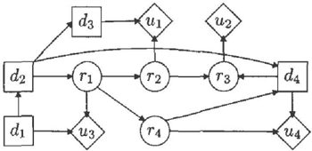
The message 1r32 is in the LP architecture computed us­ ing equation 11 which requires a total of 60 operations. In words, to compute the message 1r32, the combination of the clique potential 1r3 of clique 3 and the incoming messages from neighbours of 3 except 2 is marginalized to 2 n 3 = { r1, d2}. Thus, r2 and d4 have to be elimi­ nated from the combination of potentials 1r3, 1r13, 1f43, and

1r53. Since potentials are represented as decompositions it is possible to exploit independence relations between vari­ ables when computing messages. The domain graph G in­ duced by na, n13, 1r43, and 1r53 is shown in Fig. 3. From G it is readily seen that r2 and d4 are both probabilistic barren variables. This can be detected and exploited by the on-line triangulation algorithm. In the example, the order of elimination determined on-line when computing 1r3 2 is u =< d4, r 2 >. Since d4 is only included in 1r13 and 1r 43, d4 is eliminated from their combination and subsequently r2 is eliminated. The potential 1r32 is stored in the appro­ priate mailbox between 2 and 3.

The number of operations to perform when computing the message 1r3 2 is for each architecture shown in Tab. 2.

Table 2: The number of operations performed for each al­ gorithm when sending the message 7r32·

Algorithm	Sums	Mults	Divs	Subs	Total
S-S	88	80	4	0	164
HUGIN	32	32	8	4	76
LP	36	24	0	0	60

6.2 Architectural differences

The S-S architecture is a general architecture for infer­ ence in graphical models. It is based on the operations of marginalization and combination. Once the clique poten­ tials are initialized, they are not changed during message passing.

The HUGIN architecture is a less general architecture than the S-S architecture since it requires a division operation. During message passing the clique potentials are updated by incoming messages. The division operation is intro­ duced to avoid passing the information received from one clique back to the same clique. The update of clique poten­ tials implies that in their basic form the HUGIN architec­ ture is more efficient than the S-S architecture.

The LP architecture is based on operations of combination and marginalization. The architecture is similar to the S-S architecture in the sense that once initialized the clique po­ tentials are not updated. The representation of the clique potentials is, however, different for the two architectures. Potentials are represented as decompositions. The elimina­ tion of a variable from a subset of potentials corresponds to on-line binarization of the secondary computational struc­ ture. This is a feature which is unique to the LP architec­ ture. In the S-S and the HUGIN architectures the on-line order of elimination of variables does not have an impact on the computational requirements of computing a message. The domain graph induced by a potential is the complete graph and directions have been dropped. Therefore, the or­ der of elimination is unimportant. In the LP architecture the on-line order ofelirnination is of high importance. Poten­ tials are represented as decompositions and the direction of edges is maintained. This supports on-line exploitation of independence relations and directions of the LIMID from which the junction tree is constructed.

The LP architecture maintains decompositions of the prob­ ability and utility parts of potentials and postpone opera­ tions such that many unnecessary operations are avoided. Operations are performed during marginalization of vari­ ables and local optimization. The LP architecture may re­ quire repetition of already performed computations both when computing messages and eliminating variables. For instance, in the example the combination 1r23 0 1r13 is performed twice. It is performed when 1r34 is computed and subsequently when n35 is computed. This could be solved by binarization of the computational structure, but this increases the storage requirements. Binarization of the computational structure does not eliminate all repetitions of computations since variables are e l imi n ate d by local computation within each clique when computing messages. Thus, in order to eliminate all repetitions of computations some kind .of nested caching structure like nested junction trees (Kjrerulff (1998)), nested binary join trees (Shenoy (1997)), or a hash table of potentials is required. Binariza­ tion and nested caching structures reduce the degrees of freedom available when performing on-line triangulation. Basically, there is a time/space tradeoff with respect to the choice and granularity of the computational structure.

一

6.3 Evaluating general LIMIDs

The secondary computational structures of the S-S, HUG­ IN, and LP architectures are similar, but there are some im­ portant differences. The S-S and LP architectures use two mailboxes between each pair of neighbouring cliques to hold the most recent messages passed between the cliques. In HUG IN there is one mailbox between each pair of neigh­ bouring cliques. This mailbox contains the most recent message passed between the two neighbouring cliques. In contrast with S-S and LP architectures, the HUGIN archi­ tecture multiplies the updated policy onto the clique poten­ tial. As a consequence the HUGIN architecture is not ap­ plicable for evaluating general LIMIDs. When evaluating general LIMIDs, we may have to update each policy more than once. In this case, we initially retract the policy to be updated from the joint potential before the updated policy is computed. This is easily done in LP, and can be done in S-S if we always store the policies separately in the cliques. However, as indicated above, the HUG IN architecture can­ not retract policies, because messages are multiplied onto clique potentials during message passing.

7 Conclusion

The example LIMID ,C is not particularly complicated or has certain features. In fact, it is quite simple. Despite the simplicity of the example, there is a rather large difference in the number of operations required by each architecture to solve the LIMID. As can be seen from Tab. 1, LP offers an efficiency increase over HUGIN which offers an efficiency increase over S-S. We have compared the basic forms of the three architectures without applying any of the various speed-up techniques available (e.g. binary computational structures). This is done since each of the various speed­ up techniques known by the authors applies equally well to each of the architectures.

In this paper we have introduced three different computa­ tional architectures for solving LIMID representations of influence diagrams. The HUGIN and the LP architectures are new whereas the S-S arc h itec t ure was described in its original form in Nilsson and Lauritzen (2000). The dif­ ferences between the architectures have been described in some detail. The LP architecture offers a way to reduce both the number of operations performed and the amount of space required during message passing. The LP archi­ tecture dissolves the difference between the HUGIN and S-S architectures. Finally, see Lepar and Shenoy (1998) for a similar comparison of HUGIN and S-S propagation, and Madsen and Jensen ( 1999) for a comparison of LP, and HUGIN and S-S architectures for computing marginals of probability distributions.

Acknowledgement

Nilsson was supported by DINA (Danish Informatics Net­ work in Agricultural Sciences), funded by the Danish Re­ search Councils through their PIFT progr amm e.

References

• Dawid, A. P. (1992). Applications of a general propagation algo­ rithm for probabilistic expert systems. Statistics and Com­ puting, 2, 25�36.
• Jensen, F., Jensen, F. V., and Dittmer, S. L (1994). From influence diagrams to junction trees. In Proceedings of the lOth Con­ ference on Uncertainty in Artificial Intelligence, (ed. R. L. de Mantaras and D. Poole), pp. 367�73. Morgan Kaufmann Publishers, San Francisco, CA.
• Kjrerulff, U. (1998). Nested junction trees. In Learning in Graph­ ical Models, (ed. M. I. Jordan), pp. 51�74.
• Lauritzen, S. L. and Nilsson, D. (1999). LIMIDs of decision prob­ lems. R-99-2024, Dept. of Mathematical Sciences, Aalborg U n ive rsity. To appear in Management Science.
• Lepar, V. and Shenoy, P. P. (1998). A Comparison of Lauritzen­ Spiegelhalter, Hugin, and Shenoy-Shafer Architectures for Computing M ar g inals of Probability Distributions. In Pro­ ceedi n g s of the 14th Conference on Uncertainty in Artificail Intelligence, (ed. G. F. Cooper and S. Moral), pp. 328�37.
• Madsen, A. (1999). All Good Things Come to Those Who are Lazy. PhD thesis, Aalborg Universi t y.
• Madsen, A. L. and Jensen, F. V. (1999). Lazy p r op agat io n : A junction tree inference algorithm based on lazy evaluation. Artificial Intelligence, 113, (1-2), 203-45.
• Nilsson, D. (2001). The c om p u t a tion of moments of decompos­ able functions in probabilistic e x pert systems. In Proceed­ ings of the Third International Symposium on Adaptive Sys­ tems, pp. 116-21. Habana, CUBA.
• Nilsson, D. and Lauritzen, S. (2000). Evaluating influence dia­ grams using LIMIDs. In Proceedings of the 16th Conference on Uncertainty in Artificial Intelligence, (ed. C. Boutilier and M. Goldszmidt), pp. 436-45. Morgan Kaufmann, Stanford, California.
• Olmsted, S. (1983). On Representing and Solving Decision Prob­ lems. PhD thesis, Stanford University.
• Shachter, R. (1986). Evaluating influence diagrams. Operations Research, 34, 871�82.
• Shafer, G. and Shenoy, P. P. (1990). Pr o ba b i l i ty p ro p a g a t io n . An­ nals of Mathematics and Artificial Intelligence, 2, 327�52.
• Shenoy, P. P. (1992). Valuation-based systems for Bayesian deci­ sion analysis. Operations Research, 40, 463�84.
• Shenoy, P. P. (1997). Binary jo i n trees for computing marginals in the Shenoy-Shafer architecture. International Journal of Approximate Reasoning, 17, (2-3), 239-63.
• Shenoy, P. P. and Shafer, G. R. (1990). Axioms for pro ba bil i ty and belief-function p r o p agati on . In Uncertainty in Artificial Intelligence IV, (ed. R. D. Shachter, T. S. Levitt, L. N. Kanal, and J. F. Lemmer), pp. 169�98. North-Holland, Amsterdam.