Some Properties of Joint Probability Distributions

Marek J. Druzdzel

University of Pittsburgh Department of Information Science Pittsburgh, PA 15260 marek@lis. pitt. edu

Abstract

Several Artificial Intelligence schemes for reasoning under uncertainty explore either explicitly or implicitly asymmetries among probabilities of various states of their uncer­ tain domain models. Even though the correct working of these schemes is practically con­ tingent upon the existence of a small number of probable states, no formal justification has been proposed of why this should be the case. This paper attempts to fill this apparent gap by studying asymmetries among probabili­ ties of various states of uncertain models. By rewriting the joint probability distribu­ tion over a model's variables into a product of individual variables' prior and conditional probability distributions and applying cen­ tral limit theorem to this product, we can demonstrate that the probabilities of indi­ vidual states of the model can be expected to be drawn from highly skewed lognormal distributions. With sufficient asymmetry in individual prior and conditional probability distributions, a small fraction of states can be expected to cover a large portion of the total probability space with the remaining states having practically negligible probabil­ ity. Theoretical discussion is supplemented by simulation results and an illustrative real­ world example.

is explicated by the logical Artificial Intelligence (AI) approaches to reasoning under uncertainty - at any given point various extensions of the current body of facts are possible, one of which, although unidentified, is assumed to be true. The number of possible exten­ sion of the facts is exponential in the number of uncer­ tain variables in the model. It seems to be intuitively appealing, and for sufficiently large domains practi­ cally necessary, to limit the number of extensions con­ sidered. Several AI schemes for reasoning under un­ certainty, such as case-based or script-based reasoning, abduction (e.g., (Charniak & Shimony, 1994)), non­ monotonic logics, as well as recently proposed search­ based methods for belief updating in Bayesian belief networks (e.g., (Henrion, 1991; Poole, 1993)), seem to be following this path. If a domain is uncertain and any of the exponential number of extensions of obser­ vations is possible, one might ask why concentrating merely on a small number of them would work. In this paper, I show that we can usually expect in uncertain models a small fraction of all possible states to account for most of the total probability space.

1 INTRODUCTION

One way of looking at models of uncertain domains is that those models describe a set of possible states of the world, 1 only one of which is true. This view

1 A state can be succinctly defined as an element of the Cartesian product of sets of outcomes of all individ­ ual model's variables. There is a richness of terms used to describe states of a model: extension, instantiation, pos­ sible world, scenario, etc. Throughout this paper, I will attempt to use the term state of a model or briefly state whenever possible.

My argument refers to models rather than the systems that they describe. As argued elsewhere (Druzdzel & Simon, 1993), deriving results concerning models and relating these results to reality is the best that we can hope for as scientists. I will assume that for any uncer­ tain domain, there exists a probabilistic model of that domain, even though in some cases construction of a probabilistic model may be impractical. In all deriva­ tions and proofs, for the reasons of convenience, I will consider only discrete probability distributions. The analysis can be generalized to continuous distributions by, for example, discretizing them or considering in­ tervals over probabilities (in particular, infinitesimally small intervals). Further, I will be making certain as­ sumptions when applying centnl.l limit theorem. I be­ lieve these assumptions to be sufficiently weak to refer to the applicability of the argument as "most of the time" or "usually the case."

The remainder of this paper is structured as follows. Section 2 d es cr i b e s the probabilistic framework for rep­ resenting uncertainty, outlines my approach to study­ ing the properties of joint probability distributions

over models, and briefly discusses applicability of cen­ tral limit theorem to this analysis. Section 3 presents the main argument of the paper. Section 3.1 dis­ cusses the general case, where conditional probability distributions are arbitrary. In this case, any proba­ bility within the joint probability distribution can be expected to come from a lognormal distribution, al­ though each probability can be possibly drawn from a distribution with different parameters. It is shown that if the individual conditional probabilities are suf­ ficiently extreme, then a small fraction of the most likely states will cover most of the probability space. Section 3.2 looks at the simplest special case, where each of the conditional distributions of the model's variables is identical, showing that probabilities within the joint probability distribution are distributed log­ normally. Section 3.3 extends this result to the case where conditional distributions are not identical, but are identically distributed. Section 3.4 argues that there are good reasons to expect that the special case result may be a good approximation for most practical models. Section 4 analyzes the joint probability distri­ bution of ALARM, a probabilistic model for monitor­ ing anesthesia patients, showing empirical support for the earlier theoretical derivations. Finally, Section 5 discusses the implications of the discussed properties of uncertain domains for uncertain reasoning schemes.

2 PRELIMINARIES

2.1 PROBABILISTIC MODELS

The essence of any probabilistic model is a specifi­ cation of the joint probability distribution over the model's variables, i.e., probability distribution over all possible deterministic states of the model. It is suffi­ cient for deriving all prior, conditional, and marginal probabilities of the model's individual variables2.

Most modern textbooks on probability theory relate the joint probability distribution to the interactions among variables in a model by factorizing it, i.e., breaking it into a product of priors and condition­ als. While this view has its merits in formal expo­ sitions, it suggests viewing a probabilistic model as merely a numerical specification of a joint probability distribution that can be possibly algebraically decom­ posed into factors. This clashes with our intuition that whatever probability distributions we observe, they are a product of structural, causal properties of the domain. Causal interactions among variables in a sys­ tem determine the observed probabilistic dependences and, in effect, the joint probability distribution over all model's variables. An alternative view of a joint prob­ ability distribution is, therefore, that it is composable from rather than decomposable into prior and condi-

2 ! will often refer to the prior probability distribution over a variable as "prior" and a conditional probability distribution over a variable's outcomes given the values of other model's variables as "conditionaL"

tiona! probability distributions. In this view, each of these distributions corresponds to a causal mechanism acting in the system (Druzdzel & Simon, 1993). This reflects the process of constructing joint probability distributions over domain models in most practical sit­ uations.

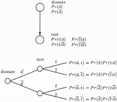
Since insight obtained from two modeling tools: Bayesian belief networks (BBNs) (Pearl, 1988) and probability trees may prove useful for the reader, I will show how they both represent a simple uncertain model involving a common activity of a clinician inter­ preting the result of a screening test for a disease. This model contains two binary variables: disease and test. The outcomes of variable disease, d and d, stand for disease present and disease absent respectively. The outcomes of variable test, t and t, stand for test posi­ tive and test negative respectively. A BEN represent­ ing this problem, shown in Figure 1, reflects the qual­ itative structure of the domain, showing explicitly de­ pendences among variables. Each variable is charac­ terized by a probability distribution conditional on its predecessors or by a prior probability distribution if the variable has no predecessors. Figure 1 shows also

a probability tree encoding the same problem. Each node in this tree represents a random variable and each branch originating from that node a possible outcome of that variable. Each complete path starting at the root of the tree and ending at a leaf corresponds to one of the four possible deterministic states of the model.

The probabilities of various states of a model can be easily retrieved in BBNs and probability trees by mul­ tiplying out the prior and conditional probabilities of individual variables. In the models of Figure 1, we multiply the priors of various outcomes of disease by the conditionals of respective outcome of test given presence or absence of disease.

2.2 STATE PROBABILITIES

Let us choose at random one state of a model that con­ sists of n variables X1, X2, X3, . . . , Xn. We choose this state equiprobably from among all possible states, regardless of its probability. One way of imagining this is that we are drawing a marble out of a basket contain­ ing uniquely marked but otherwise identical marbles. As a state is an instantiation of each of the model's n variables, another way of looking at this selection process is that we are traversing the probability tree representing the model from its root to one of its leaves taking at each step one of the possible branches with equal probability. This amounts to a random choice of one outcome from among the outcomes of each of the variables. For example, we might randomly select one of the four states in the model of Figure 1 by first choosing one of the two possible outcomes of the vari­ able disease by flipping a coin (let the outcome be for example d) and then choosing one of the two possible outcomes of the variable test by flipping a coin again (let this outcome be for example t). Our procedure made selection of each state equiprobable (with prob­ ability 0. 25 in our example). The probability p of a selected state is equal to the product of conditionals of each of the randomly selected outcomes. It is equal for our selected state to p = Pr(d, t) = Pr(d)Pr(tld). In general, if we denote Pi to be the conditional (or prior) probability of the randomly selected outcome of variable X;, we have

In random selection of a state, we chose each Pi to be one number from among the probabilities of vari­ ous outcomes of variable X;. We can, therefore, view each Pi as a random variable taking equiprobable val­ ues from among the probabilities of the outcomes of variable X;. Of course, the distribution of p; is not in general independent from the distribution of p1, i 1' j, as the outcomes of some variables may impact the conditional probability distributions of other vari­ ables. Selection of Pi within its distribution, however, is independent of any other pj, i # j. Note that in our simple example we used outcomes of independent coin tosses to choose a state. Intuitively, if the model is causal, then even though the mode in which a mech­ anism is working, described by a conditional probabil­ ity distribution, depends on the outcomes of its causal ancestors, the exact form of this distribution (i.e., the values of probabilities of different outcomes) is a prop­ erty of the mechanism and is independent on anything else in the system.

Having described the process of randomly drawing a state as above, can we say anything meaningful about the distribution of p? It turns out that we can say quite a lot about a simple transformation of p. By taking the logarithm of both sides of (1), we obtain

As for each i, p; is a random variable, its logarithm lnpi is also a random variable, albeit with a differ- ent distribution. The asymptotic behavior of a sum of random variables is relatively well understood and ad­ dressed by a class of limit theorems known collectively as central limit theorem. When the number of compo­ nents of the sum approaches infinity, the distribution of the sum approaches normal distribution, regardless of the probability distributions of the individual com­ ponents. Even though in any practical case we will be dealing with a finite number of variables, the theorem gives a good approximation even when the number of variables is small.

2.3 CENTRAL LIMIT THEOREM: "ORDER OUT OF CHAOS"

Central limit theorem (CLT) is one of the fundamen­ tal and most robust theorems of statistics, applica­ ble to a wide range of distributions. It was originally proposed for Bernoulli variables, then generalized to independent identically distributed variables, then to non-identically distributed, and to some cases where independence is violated. Extending the boundaries of distributions to which CLT is applicable is one of active areas of research in statistics. CLT is so ro­ bust and surprising that it is sometimes referred to as "order out of chaos" (de Finetti, 1974).

One of the most general forms of CLT is due to Lia­ pounov (to be found in most statistics textbooks).

Theorem 1 Let X1, X2, X3, ... , Xn be a sequence of n independent random variables such that E(Xi) = J-t i , E((X;J-t;) 2 ) =crt, and E(IX;- J-t;l3) = wr all exist for every i. Then their sum, Y = L:�=1 Xi is asymp­ totically distributed as N(E�=l J-ti, E�=l crJ), provided that

If the variables X; are identically distributed, i.e., when \ll:':i:':n J.Li = J-t, cr; = cr, and wi = w, (3) reduces to

This condition is satisfied for any distribution for which J-t and cr exist and the theorem reduces to Linde­ berg and Levy's version of CLT (also reported in most textbooks).

Returning to Equation (2), we have by the CLT, that assuming that the preconditions of CLT are satisfied, the sum on the right side is in the limit normally dis­ tributed, If lnp is normally distributed, then p itself must be drawn from a lognormal distribution.

3 PROPERTIES OF THE JOINT PROBABILITY DISTRIBUTION

CLT captures the growth of a process showing strong regularity and satisfying certain independence condi­ tions. For the purpose of this paper, I choose to

demonstrate that these conditions are reasonably sat­ isfied in the process of constructing a joint probability distribution. I will argue that the type of process that we are dealing with is one that is addressed by the theorem.

In what follows, I will be studying the properties of the logarithm of the distribution rather than the distribu­ tion itself. This is motivated by a practical consid­ eration - the lognormal distributions resulting from the application of the CLT tend to span over many orders of magnitude and are extremely skewed. Loga­ rithmic scale can be most appreciated in the diagrams that will be shown later in the paper - the skewness of the distributions makes diagrams drawn in linear scale practically unreadable. Changing the scale be­ tween logarithmic and linear is straightforward.

3.1 ARBITRARY CONDITIONAL PROBABILITY DISTRIBUTIONS

3.1.1 Preconditions

Establishing the circumstances under which the con­ dition (3) of CLT holds for multiply valued variables is not straightforward. It turns out that the condition is satisfied for propositional variables under a weak assumption, requiring only that the sequence of vari­ ances of the variables in the model is divergent in the limit.

Let a variable X; have two outcomes: x; with proba­ bility p; and outcome x; with probability 1 - p;. The mean Jl;, variance a } , and w; over the logarithm of this probability distribution are

It is clear, that for any variable i, la;l = lwd. Equa­ tion (3) transforms into

where D.; > 0 for 1 ::; i ::; n. If the sequence of variances is divergent, the denominator becomes in the limit infinitely larger than the numerator and the whole expression will approach zero, as required by (3).

3.1.2 Distribution of Probabilities of States

Let a model consist of n variables Xt, X2, X3, ... , Xn, having k1, k2, k3, . . . , kn outcomes respectively ( 1 ::; i ::; n). For any single state, we can apply the CLT to (2), viewing each p; as an independent random variable. The value of Pi will be the proba­ bility of a randomly selected outcome of variable X; ( equiprobably selected value from among the prob­ ability distribution of Xi)Let the mean and the variance of the distribution of Pi be Jli and a f re­ spectively. The logarithm of p, the probability of an individual state, obtained by multiplying priors and conditionals of individual variables is then distributed as lnp'"" N(E:1 f..L;, E�=l a l ) . The density function f(lnp) is

where 0 < p <

3.1.3 Expected Probability Mass of Various States

While f(lnp) expresses the distribution of the loga­ rithm of the probability of the randomly chosen state, a normalized pf(Inp) will express the expected con­ tribution of all states with probability p to the total probability mass (in logarithmic scale).

This function belongs the same class as f(lnp). Cis a normalizing constant that makes the integral of the function for -oo < lnp < 0 equal to 1.0.

Several important qualitative properties of this func­ tion are determined purely by its form. As E:1 a f is positive, the function is shifted with respect to f(lnp) by E7=l a? towards higher values of proba­ bilities. This shift depends on both the number of variables in the model and the individual variances in probabilities: it is stronger for distributions with high variance (i.e., distributions that show stronger asym­ metries in probabilities of various outcomes). The contribution function reaches its maximum for higher probabilities than the distribution of probabilities of states. (Exactly for lnp = E7=1 1--l i + E7 = 1 a z or for lnp = 0, whichever is lower. The zero cutoff point re­ flects the fact that the distribution is defined only for -oo < lnp < 0.) For 0::; E7=1 f..li + E�=l a ; , we will observe the pattern that a few most likely states ex­ plain most of the probability mass. Large variance in individual distributions makes, therefore, not only the

distribution of probabilities spread over many orders of magnitude but accounts for the shift of the distribu­ tion of their contributions to the total probability mass larger. The more we know about a domain, the more asymmetry individual conditionals will show. When the domain and its mechanisms are well known, prob­ ability distributions tend to be extreme. This implies a large variance and a large shift in the expected contri­ bution function and, therefore, a small number of very likely states of the model. This makes intuitive sense -we tend to act with confidence in environments that we know well, just because we can easily predict what will happen. When an environment is less familiar, the probability distributions tend to be less extreme, there is less variance in probabilities. The shift in contribu­ tion function is small and none of the states is very likely.

3.2 IDENTICAL CONDITIONAL PROBABILITY DISTRIBUTIONS

The previous section has derived limiting distribution for each individual state. Although this gives much insight into expected asymmetries in uncertain do­ mains, of more practical interest is the distribution over all probabilities of the joint probability distribu­ tion. Clearly, there are cases for which we will be able to derive these. One such special case is when the sums of means and variances of individual distribu­ tions are always the same for each state. This may be, for example, the case when all variables are indepen­ dent or when all conditional probability distributions of each of the model's variables are permutations of one another. Since we are not concerned with the out­ comes of variable X; but their probabilities, it does not matter how these probabilities are assigned to the outcomes. This special case is the subject of the cur­ rent section. The next section will relax this to the case where the conditionals for each of the variables have the same means and variances.

Let each of the random variables X; have k outcomes and let each probability Pi in (1) come from the same probability distribution (i.e., each variable's condition­ als are permutations of some discrete probability dis­ tribution over k outcomes). Since in generating the probability of a randomly selected state we choose one of the possible k outcomes of each variable equiprob­ ably, we have the mean and the variance of the dis­ tribution of each individual variable Pi in the product equal to

Since the distribution of each of the factors is the same, it is independent of other factors. Given inde­ pendence of distributions and the fact that both the mean f.l and the variance u2 exist, we can apply Linde­ berg and Levy's version of the CLT to (2), obtaining lnp""' N(nf.l, nu 2 ). The density function f(lnp) is

The normalized pf(lnp) of Equation (4), expressing the expected contribution of all states with probability p to the total probability mass becomes

As shown in Section 3.1, this function will be shifted towards higher values of probabilities, as na 2 is posi­ tive. The magnitude of this shift depends on the vari­ ances in individual probability distributions.

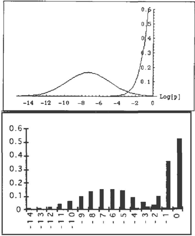
The upper diagram in Figure 2 shows this theoretically derived relationship for a model consisting of n = 10 binary (k = 2) variables with probability distributions p1 = 0.1 and P2 = 0.9. 3 Please, note that the distri­ bution of the contributions of probabilities of states to the total probability mass is strongly shifted towards higher probabilities and cut off at point logp = 0. The lower diagram in Figure 2 shows the result of a simulation in which an uncertain model satisfying the assumption was randomly created and then its joint probability distribution analyzed. This simulation was done in the spirit of a demonstration device similar to those proposed by Gauss or Kapteyn to show a mech­ anis m by which a distribution is generated. Similarity

3 This and other figures use decimal rather than n a tural logarithm because of the ease with which we can translate the value of the decimal logarithm to order of magnitude in the decimal system.

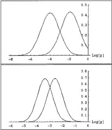
of the theoretically derived distributions to the simula­ tion results, even for as few as 10 random variables, is apparent. Figure 3 shows theoretically derived dis­ tribution functions for similar models, in which in­ dividual probability distributions were p1 = 0.2 and p2 = 0.8 (upper diagram) and Pr = 0.3 and P2 = 0. 7 (lower diagram). With smaller variances in probabili­ ties (the distributions are closer to being symmetric), the shift is much smaller. In such cases, most states will have low probabilities and, hence, no very likely states will be observed.

Since In p follows normal distribution, p will be log­ normally distributed. This distributions will usually be highly positively skewed, even for such moderate values of probabilities as 0.1. The skewness coeffi­ cient of the distribution of Figure 2, for example, is I� 7.3 X 10 7 .

Fitting a lognormal distribution with parameters E and ¢ to the distribution of probabilities within joint prob­ ability distribution allows for determining the proba­ bility threshold t for which all states less likely than t contribute totally less than fraction f of the total prob­ ability space. This threshold t can be used as an error bound in search-based belief updating algorithms. It is the solution to the following equation

This equation does not have a closed-form solution.

After solving it numerically, we can easily convert t into the fraction of states l that are less likely than t.

3.3 IDENTICALLY DISTRIBUTED CONDITIONAL PROBABILITY DISTRIBUTIONS

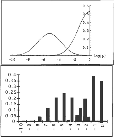
Suppose that instead of identical probabilities, we have probabilities coming from the same probability distri­ bution. Let the mean and the variance of this distribu­ tion be JJ. and rJ 2 respectively. We are still able to apply Lindeberg and Levy's version of the theorem to (2) as the distribution of each factor In Pi is independent of the distribution of any other factor. Figure 4 shows the

analogue of Figure 2 for both the theoretically derived relationship and simulation results, where the model consists of n = 10 binary (k = 2) variables with proba­ bility distributions drawn uniformly from the intervals [0,0.1] and [0.9, 1.0].

3.4 EXPECTATIONS REGARDING PRACTICAL MODELS

The general c as e result of Section 3.1, sh o w i n g t h a t e a c h p r ob a bilit y in the joint probability distribution comes f r o m a lo gn o r mal distribution, although each with perhaps different parameters, is rather conserva­ tive. In fact, CLT is known for its robustness and vio­ lations of the preconditions for the theorem may sim­ ply a ff e c t the speed of convergence ra t h e r than the nor­ mality of the sum. There are several intuitive reasons for why the distribution over probabilities of different states of a model might approach the lognormal dis­ tribution in most pra cti c a l models. Conditional pr o b ­ abilities in practical mo d e ls tend to belong to modal ranges, at most a few places after the decimal point, such as between 0.001 and 1.0. This may be an ar­ tifB-ct caused by experts' tendency to use landmark pr o b ab i liti e s that not only make various distributions modal, but also similar to one another. Another reason for this is that interactions characterized by e xtr e m el y small probabilities may be excluded from models as not relevant. Translated into the decimal logarith­ mic scale, it means the interval between -3 and 0, which is further a v erag e d over all probabilities (t h at have to add up to on e ) and for variables with few out­ comes will result in mean probabilities that belong to even more modal ranges. In effect, even though each p r o b a bilit y in the joint probability distribution comes from a di ffe r e nt lognormal distribution, the parame­ ters of these distributions may be quite close to one a not h e r . L J.L and L a2 a r e unlikely to show large vari­ ation and there will be many similar values. Topology of the model, i.e., the connectivity of the underlying g r a p h can be expected to have influence on the good­ ness of fit -as sparsely connected graphs contain less d e p e n de n c e s , they should provide a better fit. Most practical graphs seem to be sparsely connected. Fi­ nall y , the limit effects expressed by the CLT may be robust against dependences between conditional dis­ tributions of various variables. It is not unreasonable to expect that in many practical models, the distri­ bution of probabilities of the model states the joint p rob a bility distributon will approach lognormaiity.

4 EXAMPLE: ALARM

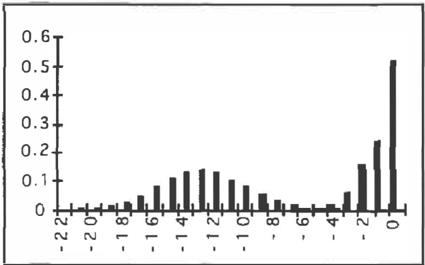
Given the strength of the conclusions of the theoret­ ical analysis, it m i gh t be useful to study the prop­ erties of the joint p r o b a b ilit y distribution over a real model. The most realistic model with a f u l l numerical specification that was available to me was ALARM, a medical d i agn o s t i c model of monitoring anesthesia patients in in te n s i v e care units (Beinlich et al., 1989). With its 38 random v ariab l e s , each having two or three outcomes, ALARM has a computationally prohibitive number of states. I se l e c t e d , therefore, several self­ contained subsets of ALARM consisting of 7 to 13 variables, and analyzed the distribution of p ro b a b il ­ ities of all states within those subsets.

Figure 5 s h o w s the result of one of such run, i d en t i ­ cal with the results of all o t h er runs with respect to the form of the observed distribution. It is a p p ar e n t that the histogram of states appears to be for nor­ mally distributed variables, which, given that the or­ dinate is in logarithmic scale, supports the the o re ti­ cally expected lognormality of the actual distribution. The histogram also indicates and small contribution of its tail to the total p r obab i lit y mass. The subset studied contained 13 va r i a bl e s , resulting in 525,312 states. The probabilities of these states were spread over 22 ord e r s of magnitude. Of all states, there was one state with probability 0.52, 10 states with proba­ bilities in the range (0.01, 0.1) and the total probability of 0.23, and 48 states with probabilities in the range (0.001, 0.01) and the total probability of 0.16. The most likely state covered 0.52 of the total probability space, the 11 most likely states covered 0.75 of the t o t a l probability space, and the 49 most likely states ( o ut of the total of 525,312) covered 0.91 of t he total probability space.

5 CONCLUSION

Using a hy po t het i c al p r o b abi l is t i c model of a. typical un c e r t a i n do ma i n , I have demonstrated that the joint probability distribution over it s variables is created by a mul t ip li ca ti ve process, c ombi n i n g conditional prob­ abilities of individual variables. Asymmetries in these individual distributions, which I argued can be ex­ pe c te d because of st r u c t ura l properties of models, re­ sult in joint probability distributions exhibiting or­ ders of magnitude differences in probabilities of var­ ious states of the model. In p ar ti c u l a r , there is usually a small fraction of states that cover a large portion of the total probability space with the remaining states having p ra c ti c a ll y ne g li gi ble p r o b a b i lit y .

Even though I referred t o m o d el s as wholes, the asym­ metries derived in the p r e c e din g sections will h o ld for their self-contained parts. Having a large probabilistic

model, we can at each reasoning step determine what, if anything, is relevant for a given query. 4 If this se­ lected part contains random variables, it is amenable to our argument.

The analysis contained in this paper concerns static systems. I believe, however, that the essential ar­ gument is easily transferable into dynamic systems. Note, that to model a transition of a system over time, we can replace each variable X in a static model by additional variables Xt, specifying the state of X at time ti. The value of variable Xt, can be specified by a probability distribution conditional on the values of variables Xt1, j < i. Then, it is straightforward to ex­ tend the argument to all newly introduced variables in the way I did for static systems.

Two special classes of interest are variables with sym­ metric probability distributions, such as the outcomes of die tosses, and deterministic variables. If all of the variables in a model had symmetric distributions or all of them were deterministic, then the denominator of (3) would be zero. Clearly, the argument will hold as long as there is a sufficient number of variables that be­ long to the complement of these two classes. Variables with symmetric distributions simply tend to shift the distribution of the probability mass towards lower val­ ues, decreasing the expected contributions of the most likely states, while deterministic variables achieve the opposite.

The significance of this analysis is that it provides a clarification for what has been long assumed but never, to my knowledge, explicated. By providing a frame­ work for studying the distribution of probabilities of individual states in the joint probability distribution, this analysis provides foundations for one direction of research on approximate reasoning schemes that are correct and yet computationally tractable. The ob­ served and theoretically derived asymmetry in the dis­ tribution of probabilities of individual states of the model suggests that considering only a small number of them can lead to good approximations in belief up­ dating. One possible reasoning scheme might consist of considering most probable states within a relevant subset of the network until the sum of the probabilities of the remaining states is below a small error thresh­ old E. Incorporation of utility considerations into such algorithm and converting it into a normatively cor­ rect decision procedure is straightforward (Druzdzel, 1993). A crucial issue in such a computation is con­ trolling for precision so that atypical symmetric mod­ els lead merely to loss of efficiency but not to incor­ rect posterior beliefs or inferior decisions. This can be accomplished by fitting a lognormal distribution to the joint probability distribution and computing the expectations based on this distribution, as shown in Section 3.2.

4(Druzdzel & Suermondt, 1994) review a variety of methods for determining relevance in the context of BBNs.

Acknowledgments

While I am solely responsible for any possible remain­ ing errors, discussions with several individuals im­ proved the above argument significantly. Feedback ob­ tained during my presentation of this work in CMU's Department of Philosophy allowed me to notice a ma­ jor flaw in an early version of the paper. Thanks to Clark Glymour, Richard Scheines, Peter Spirtes, Greg Cooper, and others for their friendly criticism. Com­ ments from Herb Simon helped in framing the argu­ ment. Anonymous reviewers provided useful feedback about the presentation.

References

• Beinlich, I., Suermondt, H., Chavez, R., & Cooper, G. (1989). The ALARM monitoring system: A case study with two probabilistic inference techniques for belief networks. In Proceedings of the Second Euro­ pean Conference on Artificial Intelligence in Medical Care (pp. 247-256). London.
• Charniak, E. & Shimony, S. E. (1994). Cost-based ab­ duction and MAP explanation. Artificial Intelligence, 66(2).
• de Finetti, B. (1974). Theory of probability. New York, NY: John Wiley & Sons.
• Druzdzel, M. J. (1993). Probabilistic reasoning in de­ cision support systems: From computation to com­ mon sense. PhD thesis, Department of Engineering and Public Policy, Carnegie Mellon University, Pitts­ burgh, PA.
• Druzdzel, M. J. & Simon, H. A. (1993, July). Causality in Bayesian belief networks. In Proceedings of the Ninth Annual Conference on Uncertainty in Artificial Intelligence (UAI-93) (pp. 3-11). Washington, D.C.
• Druzdzel, M. J. & Suermondt, H. J. (1994). Rel­ evance in probabilistic models: "backyards" in a "small world". In preparation.
• Henrion, M. (1991, July). Search-based methods to bound diagnostic probabilities in very large belief nets. In Proceedings of the Seventh Conference on Uncertainty in Artificial Intelligence (pp. 142-150). Los Angeles, CA: Morgan Kaufmann Publishers, Inc., San Mateo, CA.
• Pearl, J. (1988). Probabilistic reasoning in intelligent systems: Networks of plausible inference. San Mateo, CA: Morgan Kaufmann Publishers, Inc.
• Poole, D. (1993, July). The use of conflicts in search­ ing Bayesian networks. In Proceedings of the Ninth Annual Conference on Uncertainty in Artificial Intel­ ligence (UAI-93). Washington, D.C.