Spherical Leech Quantization for Visual Tokenization and Generation

Yue Zhao 1 , 2 Hanwen Jiang 1 , 3 Zhenlin Xu 4 , † Chutong Yang 1 Ehsan Adeli 2 , * Philipp Kr¨ ahenb¨ uhl 1 , * 1 UT Austin 2 Stanford University 3 Adobe Research 4 Mistral AI

http://cs.stanford.edu/˜yzz/npq/

simple square lattice hexagonal lattice

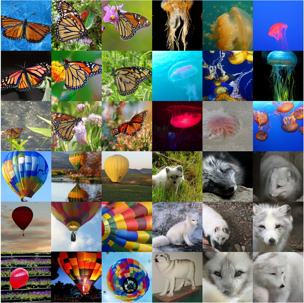
Figure 1. Upper left: A Venn Diagram that contains all definitions and quantization methods covered in this paper . We provide a unified formulation of various non-parametric quantization methods [56, 86, 91] from a lattice-coding perspective in Section 3.1. The geometric interpretation of the entropy penalties in Section 3.2 then leads to a family of densest hypersphere packing lattices (Section 3.3). Based on the spherical Leech lattice, a 24 -d case of the densest hypersphere packing lattices, we instantiate Spherical Leech Quantization ( Λ 24 -SQ) in Section 3.4 and apply it to modern discrete auto-encoders (middle) and visual autoregressive models (right). Lower left: An illustrative 2D comparison between BSQ and spherical densest-packing lattice quantization ( A 2 ). Middle: An auto-encoder with Λ 24 -SQ outperforms BSQ in image reconstruction and compression (Qualitative results on the top). Right: Qualitative and quantitative results of a visual autoregressive generation model with Λ 24 -SQ on ImageNet-1k. For the first time, we train a discrete visual autoregressive generation model with a codebook of 196 , 560 without bells and whistles and achieve an oracle-like performance .

Abstract

Non-parametric quantization has received much attention due to its efficiency on parameters and scalability to a large codebook. In this paper, we present a unified formulation of different non-parametric quantization methods through the lens of lattice coding. The geometry of lattice codes explains the necessity of auxiliary loss terms when training auto-encoders with certain existing lookup-free quantization variants such as BSQ. As a step forward, we explore a few possible candidates, including random lattices, gen-

* Equal advising.

† Work done before joining Mistral AI.

eralized Fibonacci lattices, and densest sphere packing lattices. Among all, we find the Leech lattice-based quantization method, which is dubbed as Spherical Leech Quantization ( Λ 24 -SQ), leads to both a simplified training recipe and an improved reconstruction-compression tradeoff thanks to its high symmetry and even distribution on the hypersphere. In image tokenization and compression tasks, this quantization approach achieves better reconstruction quality across all metrics than BSQ, the best prior art, while consuming slightly fewer bits. The improvement also extends to stateof-the-art auto-regressive image generation frameworks.

1. Introduction

Learning discrete visual tokenization is fundamental to visual compression [19, 29], generation [10, 27, 75], and understanding [5]. Although discrete token-based visual modeling [4, 75] follows a recipe similar to that of language modeling, we observe a paradox: Visual information carries much more data than language in quantity and diversity 1 ; However, the visual vocabulary size of vision models lags far behind that of Large Language Models (LLM) 2 . To bridge this gap, non-parametric quantization (NPQ) methods [56, 86, 91] have recently been proposed, demonstrating codebook scalability and parameter efficiency compared to vector quantization [33, 77]. However, existing NPQ methods have their own flaws and require ad hoc tweaks ( e.g ., regularization terms), which eventually boil down to the fact that most methods are heuristic and lack a principled design.

In this paper, we propose a simple and effective quantization method, called Spherical Leech Quantization ( Λ 24 -SQ), which scales to a codebook of ∼ 200 K while keeping the training of both visual tokenizers and visual autoregressive models as simple as possible. Λ 24 -SQ is theoretically grounded in the intersection of vector quantization and lattice codes. We first provide a unified formulation of existing non-parametric quantization methods from the perspective of lattice coding and reinterpret entropy penalties as a lattice relocation problem. This motivates a family of densest hypersphere packing lattices, among which the Leech lattice in the first shell [51] instantiates the codebook of Λ 24 -SQ.

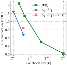
Spherical Leech Quantization features the following advantages. (i) Simplicity : Thanks to the densest sphere packing principle, Λ 24 -SQ enables the autoencoder to train with the simplest loss trio ( i.e . ℓ 1 , GAN, and LPIPS) without any regularization terms such as commitment loss and entropy penalties. (ii) Efficiency : Because of the fixed lattice vectors, Λ 24 -SQ is excluded from gradient updates, being both memory and runtime efficient. (iii) Effectiveness . Λ 24 -SQ effectively pushes the rate-distortion tradeoff frontier. Specifically, Λ 24 -SQ-based autoencoder improves rFID from 1.14 to 0.83 compared to BSQ with a slightly smaller effective bitrate ( d ⋆ = 17 . 58 vs . d = 18 ). See Figure 1.

Based on Λ 24 -SQ, we introduce improved techniques in training autoregressive visual generation models with a very large codebook. For the first time, we train a discrete visual autoregressive generation model with a codebook of ∼ 200 K , comparable to frontier language models, without bells and whistles (index subgrouping [86, 91], multihead prediction [36], bit flipping/self-correction [80], etc .) and achieve a generation FID of 1.82 FID, close to the valida-

1 Human language conveys information at several tens of bits/s [61, 69] while the brain receives visual input at 10 6 bits/s [47].

2 The tokenizer has 199,997 elements in GPT-4o [41] while 129,280 in Deepseek-R1 [34]. Meanwhile, a typical visual codebook is around 1 , 024 ∼ 16 , 384 .

tion oracle (1.78 FID) on ImageNet-1k.

2. Preliminaries

2.1. Visual tokenization and quantization

Visual tokenization. Visual tokenization transforms visual input into a set of discrete representations using an auto-encoder architecture and a bottleneck module based on vector quantization (VQ) [33, 77]. In this paper, we consider single images as input for simplicity. Given an image I ∈ R H × W × 3 and an encoder (decoder) denoted by E ( G ), we have

where p is the spatial downsample factor and the quantizer Q assigns each z ∈ Z to the closest entry k ⋆ in a learnable codebook C = [ c 1 , · · · , c K ] ∈ R K × d , i.e . ˆ z = c k ⋆ = arg min c k ∥ z -c k ∥ 2 . The entire model ( E , G , and Q ) is end-to-end trainable using approximation methods such as straight-through estimator (STE) [8], Gumbel Softmax [42], or more recent tricks like Rotation Trick [28]. One of the key challenges is to learn the codebook effectively, especially when the codebook size K increases.

Implicit codebooks. Yu et al . introduced a fixed implicit codebook C LFQ = {± 1 } d [86], where its best quantizer is binary quantization Q LFQ ( z ) = sign( z ) . Binary Spherical Quantization (BSQ) [91] further projects the hypercubeshaped codebook onto a unit sphere, i.e . C BSQ = {± 1 √ d } d . Finite Scalar Quantization (FSQ) [56] extends the codebook to multiple values per dimension i.e . ∏ d i =1 { 0 , · · · , ±⌊ L i 2 ⌋} . We refer to these implicit codebook-based methods as nonparametric quantization (NPQ) . Both LFQ and BSQ require an entropy regularization term [43] to encourage high code utilization:

where q ( z ) ≈ ˆ q ( c | z ) = exp( -τ ( c -z ) 2 ) ∑ c ∈ C LFQ exp( -τ ( c -z ) 2 ) is a soft quantization approximation [1].

Each of the NPQ variants has its own pros and cons. (1) LFQ is easiest to implement, but the computational cost for entropy increases exponentially. (2) BSQ provides an efficient approximation with a guaranteed bound, but still suffers from codebook collapse without proper entropy regularization. (3) FSQ does not need such complex regularization, but the way to obtain the number of levels per channel ( L 1 , · · · , L d ) is somewhat heuristic [56]. Although the geometric landscape of all these quantization methods varies (Figure 2 in [91]), we show in the upcoming chapter that they can be interpreted from the same lattice coding perspective. This unified formulation further motivates us to develop a novel non-parametric quantization variant that is both theoretically sound and implementation-wise easy.

Table 1. Comparisons of different non-parametric quantization methods. we overload ∏ for both scalar product and Cartesian product.

Method	LFQ [86]	FSQ [56]	BSQ [91]	F d ( N ) -SQ	Λ 24 -SQ (this paper)
Input range	R d	∏ d i =1 ( - L i 2 , L i 2 )	S d - 1	S d - 1	S 23
Code vectors	{± 1 } d	∏ d i =1 {-⌊ L i 2 ⌋ , · · · , ⌊ L i 2 ⌋}	{± 1 √ d } d	§3.3 and §A	1 √ 32 ⋃ { 2 , 3 , 4 } Λ 24 (2) s [18]
Codebook size ( |C| )	2 d	∏ d i =1 L i	2 d	N	196,560 √
Minimum distance ( d min )	2	1	2 √ d	δ min ( N )	3 2

2.2. Lattice-based codes

Lattice. A d -dimensional lattice is defined by a discrete set of points in R d that constitutes a group. In particular, the set is translated such that it includes the origin. Mathematically, an d -dimensional lattice Λ n is represented by

where G ∈ R d × d is called the generator matrix , comprising of d generator vectors g i in columns, and b ∈ Z d .

Lattice-based codes. Λ d in Eq. (3) has infinite elements by definition. In practice, we include additional constraints so that the new set is enumerable:

Particularly, spherical lattice codes [26] refers to a family of lattice-based codes with a constant squared norm, i.e . Λ d,m = { λ ∈ R d | λ = Gb , ∥ λ ∥ 2 = m } . We will see more examples in Section 3.3. Besides, we define the quantizer associated with a lattice Λ by Q Λ ( z ) = arg min t ∈ Λ ∥ z -t ∥ , which offers a bridge to vector quantization (Section 2.1).

3. Method

3.1. Non-parametric quantization as lattice coding

From the perspective of the lattice-based codes defined in Eq. (4), we can describe all variants of non-parametric quantization methods [56, 86, 91] in the same language, despite the varying geometric landscapes.

(i) Vanilla Lookup-Free Quantization [86]:

Here, e i is the standard basis vector, taking the value of 1 at the i -th index and 0 elsewhere. The constraints in Eq. (6) are equivalent to saying that λ i = ± 1 for all i .

(ii) Finite Scalar Quantization [56]: For simplicity, we consider the special case where any L i equals L .

(iii) Binary Spherical Quantization [91]:

Although it appears that Eq. (8) is simply a scaled version of Eq. (6), it is worth noting that the input range varies: z ∈ S d -1 in BSQ while z ∈ R d in LFQ.

(iv) Random-projection Quantization (RPQ) [14]. RPQ initializes the codebook { p 1 , · · · , p N } using a standard normal distribution, followed by an ℓ 2 normalization. Due to the codebook existence, strictly speaking, RPQ does not belong to lookup-free quantization by definition. Nevertheless, we can still include it in the same picture, where the generator matrix and contraints look like the following:

where G ∈ R d × N slightly abuses the definition, p i follows a projected normal distribution p i ∼ PN d (0 , I ) .

3.2. Entropy regularization as lattice relocation

Wereview the entropy regularization term from the perspective of lattice coding. We give a geometric interpretation of the entropy regularization and show that the two subterms correspond to pushing the input point towards the lattice points and finding an optimal configuration of the lattice.

Re-interpretating entropy regularization. The first term in Eq. (2) minimizes the entropy of the distribution that z is assigned to one of the codes. This means that every input should be close to one of the centroids instead of the decision boundary 3 . This becomes less of an issue since the codebook of interest is huge, exemplified by γ being greater than 1 as reported in [43, 86]. Ablation studies in BSQ [91] also reveal that we can omit E [ H [ q ( z )]] - but not H [ E [ q ( z )]] - while achieving a similar performance.

The second term maximizes the entropy of the assignment probabilities averaged over the data, which favors 'class balance' [48]. Assuming that z has a uniform distribution over its input range, we have E [ q ( z )] = P ( q ( z ) = c k ) = ∫ V k d z = | V k | , where V k is the Voronoi region for the codeword c k . H [ E [ q ( z )]] is maximized when all V k have equal volumes.

3 This principle is also known as the 'cluster assumption' [11, 32].

FSQ implicitly maximizes entropy. The interpretation explains why FSQ does not suffer from codebook collapse even without entropy penalties. Given an input z ∈ R d , FSQ first applies a bounding function f , and then rounds to the nearest integers,

Therefore, the input range is ( -L/ 2 , L/ 2) and all integer points within this range are valid lattice points 4 . The codebook size is L d , often in the range of 2 8 ∼ 2 16 . The Voronoi cell for each lattice point ˆ z is a unit-length hypercube ∏ d i =1 [ˆ z i -1 2 , ˆ z i + 1 2 ) , implicitly complying with the entropy maximization principle.

LFQ requires explicit entropy maximization. Although the Voronoi cell for each point in LFQ is also identical, the range of input and quantized output is unbounded. This breaks the uniform distribution assumption, thus requiring explicit regularization.

What's left? BSQ is missing so far. Since its input lies on a hypersphere, BSQ has to be treated separately. We will discuss the lattice relocation problem for spherical lattice codes in Section 3.3, where BSQ is one such code.

3.3. Spherical lattices and hypersphere packing

Spherical lattices. The overall pipeline is written as follows:

where norm( · ) is another way of 'bounding', and the Voronoi regions now take arbitrary shapes on the hyperspherical shell. For simplicity, we study a surrogate problem that approximates the Voronoi regions by placing N d -dimensional balls with varied radii 5 , where N is the cardinality of the lattice in which we are interested.

Entropy maximization as dispersiveness pursuit. The entropy maximization term corresponds to finding the most dispersive configuration to relocate the balls. Sloane et al . formally state this problem of placing N points on a d -dimensional sphere to maximize the minimum distance (or angle) between any pair of points in [71]. This problem generalizes the Tammes' problem [73] in dimensions greater than 3 . Mathematically, we write this max-min problem as max c 1 , ··· , c N ∈ S d -1 min 1 ≤ j<k ≤ N distance ( c j , c k ) , where we de-

︸

δ

︷︷

min

(

N

)

note δ min ( N ) for future empirical analysis.

4 When L = 2 , d = 3 , this is the well-known 'simple cubic' or 'primitive cubic' lattice in crystallography; We will see this again in Section 3.3.

5 This will leave some holes, but we believe that the total volume of holes is negligible compared to the balls.

︸

Table 2. Best known results for dense packing. The content is adapted from Table 1.1 in [18].

Dimension	1 2 3 4 5 6 7 8 12 16 24
densest packing	Z A 2 A 3 D 4 D 5 E 6 E 7 E 8 K 12 Λ 16 Λ 24

Entropy maximization as hypersphere packing. An alternative way is to assume equal radii for all hyperspheres and find the densest sphere packing [18]. The best known results in dimensions 1 to 8, 12, 16, and 24 are summarized in Table 2, where Z to E 8 and Λ 24 have been proved optimal among all lattices [16, 18].

Given these basics, we now propose a few candidates.

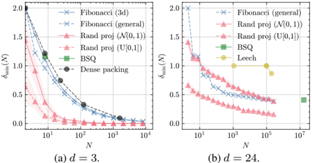
• (i) Random projection lattice follows RPQ in Section 3.1 where the projected normal distribution initializes points. We use it as a baseline to compare the dispersiveness of different candidate lattice codes in Figure 2, which turns out to be surprisingly strong in higher dimensions.
• (ii) Fibonacci lattice constructs points that 'are evenly distributed with each of them representing almost the same area' [30] in a unit square [0 , 1) 2 . We can map this point distribution to a unit-length sphere S 2 using cylindrical equal-area projection. From Figure 2a, δ min ( N ) achieved by this 3D spherical Fibonacci lattice is close to the known densest packing [71] and much better than random projection. We explore its high-dimensional generalization with the hyperspherical coordinate system inspired by [67], denoted by F d ( N ) . Construction details are left in Section A.

(iii) Densest sphere packing lattice has been introduced and summarized in Table 2. We pay particular attention to the Leech lattice Λ 24 [51]. Λ 24 can be constructed in many ways [17] and we use the most convient way to calculate. The vectors in the first shell have a minimal norm √ 32 and fall into three types; we summarize their shapes and numbers in Table 3 and provide more details in Section B. Normalizing these 196 , 560 vectors in the first shell to unit length results in the Spherical Leech Quantization ( Λ 24 -SQ) codes. We can easily get δ min ( | 1 √ 32 Λ 24 (2) s | ) = 1

Table 3. Vectors in the first shells of the Leech lattice. Λ 24 ( n ) i indicates the Leech vectors of norm 2 n (or type n and shape i ; the signs are suppressed for simplicity. The table is extracted from Table 4.13 in [18].

Class	Shape	Number	Class	Shape	Number
Λ 24 (0) 1	(0 24 )	1	Λ 24 (2) 3	(3 1 1 23 )	2 12 · 24
Λ 24 (2) 2	(2 8 0 16 )	2 7 · 759	Λ 24 (2) 4	(4 2 0 22 )	2 2 ( 24 2 )

Table 4. Comparison between the proposed Spherical Leech Quantization ( Λ 24 -SQ) and BSQ [91].

Method	BSQ [91]	Λ 24 -SQ (this paper)
Input range Code vectors	S 17 {± 1 √ 18 } 18 2 18 = 262 , 144 2 √ ≈ 0 . 471	S 23 See Table 1 196 , 560 ≈ 2 17 . 58 √ 3 ≈ 0 . 866
AR output	(1) 262 , 144 -way logits (2) 18 × binary logits
Codebook size
δ min ( |C| )	18	2
		(1) 196 , 560 -way logits (2) 24 × nonary logits
Self-correct	bitwise flip	9 -itwise toggle

for s = 2 , 3 , 4 and δ min ( | 1 √ 32 ⋃ { 2 , 3 , 4 } Λ 24 (2) s | ) = √ 3 2 . From Figure 2b, δ min ( N ) is much larger than all other candidates.

BSQ are not the densest packing lattice codes. Before we conclude this chapter, we compare Λ 24 -SQ with BSQ, the prior art, in Table 4. Since the codebook size takes log 2 (196 , 560) ≈ 17 . 58 bits, we use BSQ with d = 18 . Λ 24 -SQ increases δ min ( |C| ) by more than 80% ( 0 . 471 → 0 . 866 ), indicating its superiority. Empirical results in Section 5 also support that Λ 24 -SQ enables a simple loss design such that the entropy regularization term can be omitted. Comparing Figures 2a and 2b, we also conclude that the improvement in δ min ( |C| ) of BSQ over the random lattice baseline decreases when d increases.

3.4. Spherical Leech Quantization in practice

Instantiation. Λ 24 -SQ follows the pipeline of Eq. (11) with the lattice being 1 √ 32 ⋃ { 2 , 3 , 4 } Λ 24 (2) s . Despite the huge codebook size, because the lattice vectors are fixed, we can use tiling and JIT-compiling techniques to reduce both memory and runtime costs compared to vanilla VQ.

Accomodating smaller codebooks. In some cases with less data, a codebook size of 196 , 560 may be too large. We can also take one type of Λ 24 (2) s or its subset so that the codebook size range 1 , 104 ∼ 98 , 304 .

3.5. Integration with other quantization techniques

Multi-scale residual quantization. Since Λ 24 -SQ is an inplace replacement of VQ, we can use it in combination with other techniques, such as multiscale quantization [45] and residual quantization [6, 50]. In this paper, we integrate Λ 24 -SQ into the VAR tokenizer [75] for image generation, allowing for direct comparison with quantization methods such as VQ in VAR [75] and BSQ in Infinity [36].

Aligning with vision foundation models. Better reconstruction does not always lead to better generation quality [35, 56, 63, 86]. VAVAE [77] proposes to address this reconstruction-generation dilemma by aligning latent embeddings with vision foundation models. We use the VF loss [84] between the latent embedding before quantization and the feature extracted from a pretrained DINOv2 [58].

4. Autoregression with a Very Large Codebook

4.1. Representing the codebook mapping

Preliminaries. As NPQ scales up the effective size of the codebook, effectively representing the codebook mapping for the autoregressive models becomes a big issue. The most straightforward way is to represent each code by a unique index. It uses an embedding matrix E ∈ R | V |× D to map each index to a vector and an unembedding matrix E ′ ∈ R D ×| V | to get the final logits of dimension | V | for a simple classification problem. Memory cost and training stability are the two biggest challenges.

There are two more solutions: (1) index subgroup [86] and (2) bitwise operation [36, 80]. The former is compatible with the autoregression framework, but the resulting sequence length grows linearly w.r.t. the number of groups. Han et al . model bitwise tokens with multiple BCE losses in parallel in [36]. However, it only applies to LFQ/BSQ and relies on bitwise self-correction to mitigate the train-test discrepancy. In the following, we show our improvements to accommodate the family of spherical lattice codes.

Simple classification with memory optimization. We adopt the cut cross entropy (CCE) [81] to address memory consumption. Since the visual auto-regressive models are trained from scratch, we use Kahan summation [46] to maintain numerical stability, as suggested by [81]. We leave the training techniques in Section 4.2.

Factorized d -itwise prediction. Densest sphere-packing lattices like E 8 and Λ 24 take integer values, but all possible values go beyond binary [91]. We generalize the concept of bitwise prediction and propose a factorized d -it 6 prediction. Assuming independence across channels, the joint log-probability of one lattice code c (1: d ) is approximated by the sum of the log-probabilities of each dimension, i.e .

where p ( c ( i ) ) denotes the probability of the i -th element of

6 Short for log based unit , analogous to bit for log 2 () and nat for ln() .

the d -dim lattice codes. For Λ 24 -SQ, we use 24 9 -way classification heads to include all possible values {-4 , · · · , 4 } . d -itwise self-correction is also possible by toggling any element with a certain probability, though we do not explore it in this paper.

4.2. Training

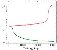
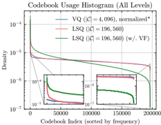
We train a 16-layer Infinity model but observe a consistent increase in gradient norms and explosion of loss (the blue curve in Figure 3 7 ). A natural hypothesis for this is about the large codebook 8 : We plot the codebook usage on ImageNet-val, sorted by density, in Figure 4. For the standard VQ codebook, the largest frequency and smallest frequency are within the same order of magnitude ( 7 . 69 e -4 1 . 37 e -4 ≈ 5 . 6 ). For Λ 24 -SQ's large codebook, the ratio between the most frequent index and the least frequent one surges to 8 . 90 e -5 2 . 41 e -6 ≈ 37 . The imbalance is more visible after the VF alignment (Sec. 3.5). We further hypothesize that it prevents prior visual auto-regressive models from utilizing a large visual codebook for generation, although the low utilization problem during reconstruction appears to be fixed [70, 93].

Despite the difficulty, we recognize that this is not a unique issue in visual generation. An unbalanced, large codebook is common when training large language models [15, 57, 82]. Therefore, we borrow two simple and effective techniques, namely Z-loss [15] and improved optimization with orthonormalized matrix updates [44, 52].

Z-loss [15] prevents the final output logits from exploding. Namely, L Z = α | log Z | 2 = α ∣ ∣ ∣ log ( ∑ V i exp( z i ) )∣ ∣ ∣ 2 , where we set α to be 10 -4 as in [57].

7 The loss explosion occurs earlier when the model goes to 1B.

8 Also, we drop the entropy regularization that promotes class balance.

2

|

Z

log

|

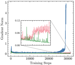
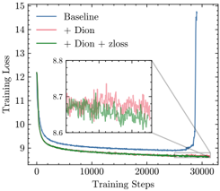
Figure 3. Training curve for a 16-layer ∞ -CC model. The Dion optimizer addresses the problem of exploding gradient norm. Z-loss effectively regularizes | log Z | 2 and smoothens the loss and gradient curve, leading to a lower training loss.

Distributed Orthonormalized Updates . We use Dion optimizer [2] for all weight tensors greater than 1D and Lion [13] for 1D weight tensors and the [un]embedding layers. The unembedding layer is updated with a learning rate scaled by 1 / √ d in , where d in is its input dimension.

From Figure 3, both techniques lead to smoother training dynamics, with lower variance and fewer spikes, and achieve a lower final loss value.

4.3. Sampling

The sampling follows convention [75]. We apply classifierfree guidance (CFG), first proposed for diffusion models [38] and later adopted in AR-based models [56, 72]. At inference, each token's logit z g is formed by z g = z u + s ( z c -z u ) , where z c is the conditional logit, z u is the unconditional logit, and s is the CFG scale. We use layerwise linearly scaling CFG, first introduced in Infinity [36]. We observe that linearly scaling topK is also helpful. For the factorized d -itwise configuration, we apply CFG on the normalized probability, i.e . p g = p u + s ( p c -p u ) , where p · = exp ( ∑ d i log p · ( c ( i ) ) ) according to Eq. (12). Nucleus sampling (top p ) [39] is also used.

5. Experiments

5.1. Experimental setup

Architectures. We train the image tokenizer with different quantization methods on ImageNet-1K [66]. The experiments cover two network architectures: (1) Vision Transformers (ViT) [24], which runs at a high throughput and yields high reconstruction fidelity, and (2) ConvNets, which are more commonly seen in image generation. We compare our method with VQ-based [65, 75] and BSQ-based methods [36]. The training details are specified in the Appendix. Training objectives. We use a weighted average of three losses, the mean absolute error (MAE, ℓ 1 ), GAN, and perceptual loss, without any other regularization terms. The MAE, GAN, and perceptual loss optimize the PSNR, FID, and LPIPS score according to their respective definitions. Therefore, this trio can no longer be simplified.

Evaluation. We evaluate image compression in the Kodak Lossless True Color Image Suite. It includes 24 24bit lossless color PNG images. We report PSNR and MS-

Table 5. Image reconstruction results on COCO2017 and ImageNet-1k ( 256 × 256 ).

					COCO2017 val				ImageNet-1k val
Method	Arch.	Quant.	Param.	#bits TP ↑	PSNR	↑	SSIM ↑	LPIPS ↓	rFID ↓	PSNR ↑	SSIM ↑	LPIPS ↓ rFID ↓
DALL-E dVAE [64]	C	VQ	98M	13 34.0	25.15 ± 3.49	.7497 ± .1124	.3014 ±	.1221	55.07 25.46 ±	3.93	.7385 ± .1343	.3127 ± .1480	36.84
MaskGIT [10]	C	VQ	54M	10 37.6	17.52 ± 2.75	.4194 ± .1619	.2057 ±	.0473	8.90 17.93 ±	2.93	.4223 ± .1827	.2018 ± .0543	2.23
SD-VAE 1.x [65]	C	VQ	68M	14 22.4	22.54 ± 3.55	.6470 ± .1409	.0905 ±	.0323	6.07 22.82	± 3.97	.6354 ± .1644	.0912 ± .0390	1.23
ViT-VQGAN [85]	T	VQ	182M	13 † 7.5		-	-	-	-	-	-	-	1.55
BSQ-ViT [91]	T	BSQ	174M	18 45.1	25.08 ± 3.57	.7662 ±	.0993 .0744 ±	.0295	5.81	25.36 ± 4.02	.7578 ± .1163	.0761 ± .0358	1.14
Λ 24 -SQ-ViT	T	Λ 24 -SQ	174M	⪅ 18 45.1	26.00 ± 3.67	.8008 ±	.0879 .0632 ±	.0262	5.15 26.37 ±	4.15	.7934 ± .1011	.0622 ± .0317	0.83

Table 6. Image compression on Kodak. Λ 24 -SQ † use only ℓ 1 loss and does not use arithmetic coding.

Method	BPP ↓	PSNR ↑	MS-SSIM ↑
JPEG2000	0.2986	29.192	.9304
WebP	0.2963	29.151	.9396
MAGVIT2	0.2812	23.467	.8452
BSQViT	0.2812	27.785	.9481
Λ 24 -SQ †	0.2747	29.632	.9637

SSIM [79] at different levels of bits per pixel (BPP). We assess image reconstruction and generation on the ImageNet1k validation set. Reconstruction is measured by FID, PSNR, SSIM, and LPIPS [90]. Generation is measured by FID, Inception Score (IS) [68], and improved precision and recall (IPR) [49], calculated by the ADMTensorflow Evaluation Suite [23]. We use rFID/gFID to disambiguate.

5.2. Main results: Comparison to state-of-the-art

State-of-the-art image reconstruction. Table 5 compares the image reconstruction results on COCO 2017 and ImageNet-1k. A ViT-based auto-encoder with Λ 24 -SQ reduces rFID by 10 ∼ 20% and improves all other metrics.

State-of-the-art image compression. We show the compression results on Kodak in Table 6. Since the resolution is 768 × 512 or 512 × 768 , we encode/decode them in 256 × 256 tiles without overlapping or padding. We compare our method with traditional codecs, including JPEG2000 [22] and WebP [31], and tokenizer-based approaches, including MAGVITv2 [86] and BSQViT [91]. Λ 24 -SQ-ViT achieves higher PSNR and MS-SSIM scores while using a slightly smaller BPP. Note that the rate-distortion tradeoff can be further improved ( ∼ 25% less bitrate) by training an unconditional AR model for arithmetic coding [21, 91], which is not the primary focus of this paper.

State-of-the-art image generation. We select the class-

Table 7. Image generation on ImagetNet. ( re ) refers to rejection sampling.

Method	gFID ↓	IS ↑	Prec ↑	Rec ↑ # Params		Steps
VQGAN ( re ) [27]	5.20	280.3	-	-	1.4B	256
VIM ( re ) [85]	3.04	227.4	-	-	1.7B	1024
RQ-TF ( re ) [50]	3.80	323.7	-	-	3.8B	68
LlamaGen [72]	3.05	222.3	0.80	0.58	3.1B	256
VAR- d 24 [75]	2.09	312.9	0.82	0.59	1.0B	10
∞ -CC+ Λ 24 -SQ	2.18	332.3	0.78	0.63	1.0B (0.3B)	7
VAR- d 30 [75]	1.92	323.1	0.82	0.59	2.0B	10
∞ -CC+ Λ 24 -SQ	1.82	333.4	0.78	0.64	2.8B (0.4B)	7
(Val data)	1.78	236.9	0.75	0.67	-	-

conditioned Infinity [36] as a baseline. Infinity-CC employs a 7-level next-scale prediction backbone, saving ∼ 25% tokens and running ∼ 30% faster than V AR (10 levels) [75]. (i) VAR tokenizer. We train a VAR tokenizer with the standard schedule (100 epochs) suggested in Infinity [36]. We use Λ 24 -SQ as the bottleneck with two codebook sizes: (1) a complete codebook, whose bitrate is similar to BSQ ( d = 18 ), and (2) a subset of 16,384 codes, whose bitrate is equivalent to BSQ ( d = 14 ). Figure 5 clearly demonstrates the superiority of our method.

(ii) VAR generation. Table 7 shows the generation results on ImageNet-1k. We also provide the oracle result computed from the validation set in the bottom row. InfinityCC+ Λ 24 -SQ works comparably with VARd 24 in terms of model size (1B) while being 30% more efficient. Note that our results achieve a higher recall and push the precisionrecall tradeoff closer to the validation oracle. We attribute this to the larger codebook, which better captures visual diversity. When the parameters increase to 2.8B, ∞ -CC+ Λ 24 -SQ achieves an FID of 1.82, which is comparable to both VARd 30 and the oracle result.

5.3. Scientific investigations and ablative studies

Dispersiveness leads to better rate-distortion tradeoff. We start from the comparison in Figure 2 and ask if dispersiveness, quantified by higher δ min ( N ) , leads to better rate-distortion tradeoff for visual tokenization . We train a plain ViT-small encoder-decoder on ImageNet128 × 128

|C|

Table 8. Quantizer with higher δ min lead to better reconstruction. VQ ( PN -): projected normal distribution initialization. Note that we gray out the last two rows to indicate that the learnable configurations are not used elsewhere.

	Method	|C|	Utility ↑	rFID ↓	LPIPS ↓	SSIM ↑	PSNR ↑
	VQ (RP, U )	2 14	95.09%	13.08	0.1080	0.7086	23.018
	VQ (RP, N )	2 14	100.0%	12.00	0.1021	0.7240	23.354
	BSQ	2 14	97.21%	12.98	0.1048	0.7058	23.171
	Λ 24 -SQ	2 14	100.0%	11.16	0.1007	0.7258	23.390
	BSQ	2 17	57.04%	12.46	0.0963	0.7296	23.742
	BSQ	2 18	70.00%	10.96	0.0914	0.7351	23.752
	VQ (RP, N )	196 , 560	94.87%	9.10	0.0829	0.7624	24.216
	Λ 24 -SQ	196 , 560	94.84%	8.98	0.0811	0.7647	24.282
(Learn)	VQ ( PN -init.)	196 , 560	95.45%	9.13	0.0832	0.7623	24.226
	Λ 24 -SQ	196 , 560	94.78%	8.78	0.0820	0.7644	24.274

Pred. head gFID ↓			IS ↑	Prec ↑	Rec ↑
BSQ [36]	BCE	10.7	219.6	0.85	0.21
BSQ [36]	CE	10.3	187.3	0.85	0.27
Λ 24 -SQ	9-way CE	11.7	155.8	0.82	0.29
Λ 24 -SQ	CE	8.7	215.4	0.85	0.30

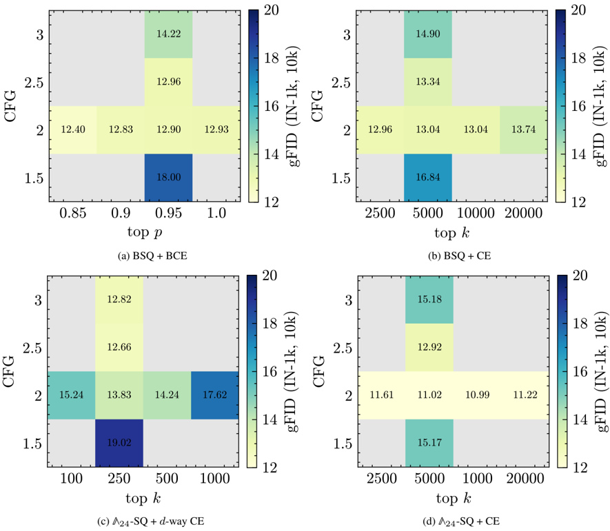
Table 9. ∞ -CC with different prediction heads. CFG = 2 , p = 0 . 95 , and K varies. Grid search in Figure 8.

while varying only the quantization bottleneck. We also test two vocabulary sizes, medium ( 2 14 ) and large ( 196 , 560 ). With the codebook fixed, we find Λ 24 -SQ achieves the best rFID, LPIPS, SSIM, and PSNR. The random projection VQ and BSQ follow behind. We also test learnable codebooks given these as initialization. The conclusion still holds, and a learnable codebook does not greatly affect the final results.

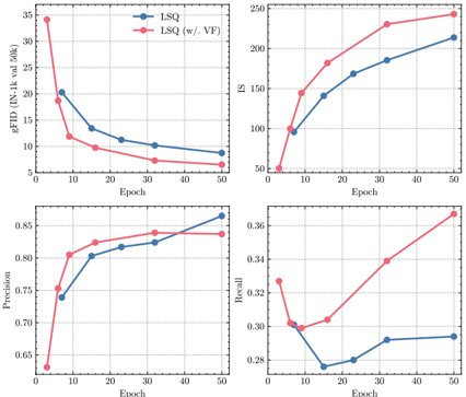
VF alignment helps discrete tokens, too. Figure 5 shows a worse reconstruction quality after aligning with the DINOv2 feature [58]. However, Figure 6 demonstrates that the VAR generation using a VF-aligned tokenizer converges faster and achieves better final results in gFID, IS, and especially recall. This extends the findings in V A V AE [84] about VF alignment from continuous latents to discrete ones.

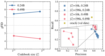
VAR generation with different heads. We test various prediction heads, namely 18 × BCE vs . 262 , 144 -way CE for ∞ -CC+BSQ, 24 × 9-way CE vs . 196 , 560 -way CE for ∞ -CC+ Λ 24 -SQ in Table 9, showing that Λ 24 -SQ +CE achieves great results despite simplicity. The factorized d -itwise prediction yields worse gFID and lower recall in both cases, implying that factorized approximation sacrifices diversity . Wealso find that the optimal sampling hyperparameters vary and conduct a small-scale grid search in Figure 8. Scaling the codebook size does matter. The last but not least critical question is whether increasing the codebook size benefits the generation results . To answer this, we used the two VAR tokenizers with C = 196 , 560 vs . 16 , 384 ) with reconstruction results in Figure 5, and trained V AR models with varied sizes on top while keeping all the rest settings the same. To report the gFID, we search the sampling hy-

|C|

perparameters to find an optimal value. From Figure 7, we conclude that increasing the codebook size improves gFID when the model is large, e.g ., 12-layer (0.24B) to 16-layer (0.49B). This echoes the finding in LLMs that larger models deserve larger vocabularies [74]. We look at the improved precision and recall metric in the right subplot of Figure 7. We use topp = 0 . 95 , CFG of lin(1 , 0 . 33) , and vary topk to obtain the data points. We find that when the codebook size increases, the precision-recall Pareto frontier moves towards the oracle precision-recall derived from the val set.

6. Related work

Vector quantization (VQ) [33, 77] lays the foundations of learning discrete visual tokens. However, VQ is notoriously difficult to train, which is attributed to the misalignment between the embedding distribution of the model and the codebook [40]. Optimization tricks are then introduced, e.g . Gumbel Softmax [3, 42], Rotation trick [28], and Index

Backpropagation [70]. The line of lattice-based quantization methods covered in this paper [56, 86, 91] addresses this misalignment issue by keeping the codebook fixed. Our Λ 24 -SQ is an intuitive extension in this direction.

Scaling visual tokenizers has recently attracted attention and covers many directions, including increasing parameters [83], training data [37], unifying generation and understanding [55, 92], and encoding multiple modalities [54, 78]. Our paper focuses on scaling the vocabulary size. Despite several advances in reconstruction [70, 93], none have reported that an expanded vocabulary benefits generation yet. Our paper shows that a visual autoregressive model scales to a very large codebook ( ∼ 200 K ) without tricks such as index subgrouping [86], etc .

Autoregressive visual generation applies an autoregressive model to visual generation [12, 25, 76] similar to the LLM paradigm [7, 9, 62]. Modern AR model employs a visual tokenizer for efficiency [27]. Subsequent work explores what to auto-regress [75, 87] and auto-regressive order [59, 88]. Most AR models are based on a medium-sized visual vocabulary ( 1 K ∼ 10 K ), limiting their potential [86].

Lattice coding has wide applications in digital communication [89] and cryptography [60]. In this paper, we borrow this concept to describe different non-parametric quantization methods and others in the same language. This further inspires us to devise new quantization methods based on the principle of densest hypersphere packing . The hyperspherical prior is also loosely related to some recent work about learning on a spherical manifold [20, 53].

7. Conclusion

We have introduced spherical Leech quantization ( Λ 24 -SQ), a novel quantization method that scales the visual codebook to ∼ 200 K , and demonstrated its applications in visual compression, reconstruction, and generation on ImageNet. In the future, we are interested in verifying its effectiveness in larger-scale settings, e.g ., text-conditioned visual generation.

Acknowledgments. This material is based upon work in part supported by the National Science Foundation under Grant No. IIS-1845485. The authors acknowledge the IFML Center for Generative AI and the Texas Advanced Computing Center (TACC) at The University of Texas at Austin for providing computational resources that have contributed to the research results reported within this paper. This work was supported by a Hoffman-Yee Research Grant from the Stanford Institute for Human-Centered Artificial Intelligence (HAI). This research was also supported in part by Lambda, Inc. YZ would like to thank Jeffrey OuyangZhang and Mi Luo for their help in setting up environments on TACC; Yi Jiang and Bin Yan for their clarification on VAR and Infinity baselines.

References

1. Eirikur Agustsson, Fabian Mentzer, Michael Tschannen, Lukas Cavigelli, Radu Timofte, Luca Benini, and Luc V Gool. Soft-to-hard vector quantization for end-to-end learning compressible representations. NeurIPS , 2017. 2
2. Kwangjun Ahn, Byron Xu, Natalie Abreu, Ying Fan, Gagik Magakyan, Pratyusha Sharma, Zheng Zhan, and John Langford. Dion: Distributed orthonormalized updates. arXiv preprint arXiv:2504.05295 , 2025. 6
3. Alexei Baevski, Steffen Schneider, and Michael Auli. vqwav2vec: Self-supervised learning of discrete speech representations. In ICLR , 2020. 8
4. Yutong Bai, Xinyang Geng, Karttikeya Mangalam, Amir Bar, Alan L Yuille, Trevor Darrell, Jitendra Malik, and Alexei A Efros. Sequential modeling enables scalable learning for large vision models. In CVPR , 2024. 2
5. Hangbo Bao, Li Dong, Songhao Piao, and Furu Wei. Beit: Bert pre-training of image transformers. In ICLR , 2022. 2
6. Christopher F Barnes, Syed A Rizvi, and Nasser M Nasrabadi. Advances in residual vector quantization: A review. TIP , 1996. 5
7. Yoshua Bengio, R´ ejean Ducharme, Pascal Vincent, and Christian Jauvin. A neural probabilistic language model. JMLR , 2003. 9
8. Yoshua Bengio, Nicholas L´ eonard, and Aaron Courville. Estimating or propagating gradients through stochastic neurons for conditional computation. arXiv preprint arXiv:1308.3432 , 2013. 2
9. Tom Brown, Benjamin Mann, Nick Ryder, Melanie Subbiah, Jared D Kaplan, Prafulla Dhariwal, Arvind Neelakantan, Pranav Shyam, Girish Sastry, Amanda Askell, et al. Language models are few-shot learners. NeurIPS , 2020. 9
10. Huiwen Chang, Han Zhang, Lu Jiang, Ce Liu, and William T Freeman. Maskgit: Masked generative image transformer. In CVPR , 2022. 2, 7
11. Olivier Chapelle and Alexander Zien. Semi-supervised classification by low density separation. In AISTATS , 2005. 3
12. Mark Chen, Alec Radford, Rewon Child, Jeffrey Wu, Heewoo Jun, David Luan, and Ilya Sutskever. Generative pretraining from pixels. In ICML , 2020. 9
13. Xiangning Chen, Chen Liang, Da Huang, Esteban Real, Kaiyuan Wang, Hieu Pham, Xuanyi Dong, Thang Luong, Cho-Jui Hsieh, Yifeng Lu, et al. Symbolic discovery of optimization algorithms. NeurIPS , 2023. 6
14. Chung-Cheng Chiu, James Qin, Yu Zhang, Jiahui Yu, and Yonghui Wu. Self-supervised learning with randomprojection quantizer for speech recognition. In ICML , 2022. 1, 3
15. Aakanksha Chowdhery, Sharan Narang, Jacob Devlin, Maarten Bosma, Gaurav Mishra, Adam Roberts, Paul Barham, Hyung Won Chung, Charles Sutton, Sebastian Gehrmann, et al. Palm: Scaling language modeling with pathways. JMLR , 24(240):1-113, 2023. 6
16. Henry Cohn, Abhinav Kumar, Stephen Miller, Danylo Radchenko, and Maryna Viazovska. The sphere packing problem in dimension 24. Annals of mathematics , 2017. 4

1. John Horton Conway and Neil JA Sloane. Twenty-three constructions for the leech lattice. Proceedings of the Royal Society of London. A. Mathematical and Physical Sciences , 381 (1781):275-283, 1982. 4
2. John Horton Conway and Neil James Alexander Sloane. Sphere packings, lattices and groups . Springer Science & Business Media, 2013. 3, 4, 5, 2
3. Thomas J Daede, Nathan E Egge, Jean-Marc Valin, Guillaume Martres, and Timothy B Terriberry. Daala: A perceptually-driven next generation video codec. arXiv preprint arXiv:1603.03129 , 2016. 2
4. Tim R Davidson, Luca Falorsi, Nicola De Cao, Thomas Kipf, and Jakub M Tomczak. Hyperspherical variational autoencoders. In UAI , 2018. 9
5. Gr´ egoire Del´ etang, Anian Ruoss, Paul-Ambroise Duquenne, Elliot Catt, Tim Genewein, Christopher Mattern, Jordi GrauMoya, Li Kevin Wenliang, Matthew Aitchison, Laurent Orseau, et al. Language modeling is compression. In ICLR , 2024. 7
6. Antonin Descampe, David Tschumperl´ e, Gilles Burel, Charles Deledalle, Pierre A. Carr´ e, and Benoit Macq. Openjpeg - an open-source jpeg 2000 codec written in C. In PCS , 2006. 7
7. Prafulla Dhariwal and Alexander Nichol. Diffusion models beat gans on image synthesis. NeurIPS , 2021. 7
8. Alexey Dosovitskiy, Lucas Beyer, Alexander Kolesnikov, Dirk Weissenborn, Xiaohua Zhai, Thomas Unterthiner, Mostafa Dehghani, Matthias Minderer, Georg Heigold, Sylvain Gelly, et al. An image is worth 16x16 words: Transformers for image recognition at scale. In ICLR , 2021. 6
9. Alexei A Efros and Thomas K Leung. Texture synthesis by non-parametric sampling. In ICCV , 1999. 9
10. Thomas Ericson and Victor Zinoviev. Codes on Euclidean spheres . Elsevier, 2001. 1, 3
11. Patrick Esser, Robin Rombach, and Bjorn Ommer. Taming transformers for high-resolution image synthesis. In CVPR , 2021. 2, 7, 9
12. Christopher Fifty, Ronald G Junkins, Dennis Duan, Aniketh Iyengar, Jerry W Liu, Ehsan Amid, Sebastian Thrun, and Christopher R´ e. Restructuring vector quantization with the rotation trick. In ICLR , 2025. 2, 8
13. Allen Gersho and Robert M Gray. Vector quantization and signal compression . Springer, 2012. 2
14. ´ Alvaro Gonz´ alez. Measurement of areas on a sphere using fibonacci and latitude-longitude lattices. Mathematical geosciences , 42(1):49-64, 2010. 4, 1
15. Google Developers. WebP Compression Techniques. https : / / developers . google . com / speed / webp/docs/compression , 2025. Accessed: 2025-1010. 7
16. Yves Grandvalet and Yoshua Bengio. Semi-supervised learning by entropy minimization. NeurIPS , 2004. 3
17. Robert Gray. Vector quantization. IEEE ASSP Magazine , 1 (2):4-29, 1984. 2, 8
18. Daya Guo, Dejian Yang, Haowei Zhang, Junxiao Song, Peiyi Wang, Qihao Zhu, Runxin Xu, Ruoyu Zhang, Shirong Ma, Xiao Bi, et al. Deepseek-r1 incentivizes reasoning in llms
19. through reinforcement learning. Nature , 645(8081):633638, 2025. 2
20. Agrim Gupta, Lijun Yu, Kihyuk Sohn, Xiuye Gu, Meera Hahn, Fei-Fei Li, Irfan Essa, Lu Jiang, and Jos´ e Lezama. Photorealistic video generation with diffusion models. In ECCV , 2024. 5
21. Jian Han, Jinlai Liu, Yi Jiang, Bin Yan, Yuqi Zhang, Zehuan Yuan, Bingyue Peng, and Xiaobing Liu. Infinity: Scaling bitwise autoregressive modeling for high-resolution image synthesis. In CVPR , 2025. 2, 5, 6, 7, 8, 3
22. Philippe Hansen-Estruch, David Yan, Ching-Yao Chung, Orr Zohar, Jialiang Wang, Tingbo Hou, Tao Xu, Sriram Vishwanath, Peter Vajda, and Xinlei Chen. Learnings from scaling visual tokenizers for reconstruction and generation. In ICML , 2025. 9
23. Jonathan Ho and Tim Salimans. Classifier-free diffusion guidance. In NeurIPS workshop , 2022. 6
24. Ari Holtzman, Jan Buys, Li Du, Maxwell Forbes, and Yejin Choi. The curious case of neural text degeneration. In ICLR , 2020. 6
25. Minyoung Huh, Brian Cheung, Pulkit Agrawal, and Phillip Isola. Straightening out the straight-through estimator: Overcoming optimization challenges in vector quantized networks. In ICML , 2023. 8
26. Aaron Hurst, Adam Lerer, Adam P Goucher, Adam Perelman, Aditya Ramesh, Aidan Clark, AJ Ostrow, Akila Welihinda, Alan Hayes, Alec Radford, et al. Gpt-4o system card. arXiv preprint arXiv:2410.21276 , 2024. 2
27. Eric Jang, Shixiang Gu, and Ben Poole. Categorical reparameterization with gumbel-softmax. In ICLR , 2017. 2, 8
28. Aren Jansen, Daniel PW Ellis, Shawn Hershey, R Channing Moore, Manoj Plakal, Ashok C Popat, and Rif A Saurous. Coincidence, categorization, and consolidation: Learning to recognize sounds with minimal supervision. In ICASSP , 2020. 2, 3
29. Keller Jordan, Yuchen Jin, Vlado Boza, Jiacheng You, Franz Cesista, Laker Newhouse, and Jeremy Bernstein. Muon: An optimizer for hidden layers in neural networks, 2024. 6
30. Biing-Hwang Juang and A Gray. Multiple stage vector quantization for speech coding. In ICASSP , 1982. 5
31. William Kahan. Pracniques: further remarks on reducing truncation errors. Communications of the ACM , 8(1):40, 1965. 5
32. Kristin Koch, Judith McLean, Ronen Segev, Michael A Freed, Michael J Berry, Vijay Balasubramanian, and Peter Sterling. How much the eye tells the brain. Current biology , 16(14):1428-1434, 2006. 2
33. Andreas Krause, Pietro Perona, and Ryan Gomes. Discriminative clustering by regularized information maximization. NeurIPS , 2010. 3
34. Tuomas Kynk¨ a¨ anniemi, Tero Karras, Samuli Laine, Jaakko Lehtinen, and Timo Aila. Improved precision and recall metric for assessing generative models. NeurIPS , 2019. 7
35. Doyup Lee, Chiheon Kim, Saehoon Kim, Minsu Cho, and Wook-Shin Han. Autoregressive image generation using residual quantization. In CVPR , 2022. 5, 7

1. John Leech. Notes on sphere packings. Canadian Journal of Mathematics , 19:251-267, 1967. 2, 4
2. Jingyuan Liu, Jianlin Su, Xingcheng Yao, Zhejun Jiang, Guokun Lai, Yulun Du, Yidao Qin, Weixin Xu, Enzhe Lu, Junjie Yan, et al. Muon is scalable for llm training. arXiv preprint arXiv:2502.16982 , 2025. 6
3. Ilya Loshchilov, Cheng-Ping Hsieh, Simeng Sun, and Boris Ginsburg. ngpt: Normalized transformer with representation learning on the hypersphere. In ICLR , 2025. 9
4. Jiasen Lu, Liangchen Song, Mingze Xu, Byeongjoo Ahn, Yanjun Wang, Chen Chen, Afshin Dehghan, and Yinfei Yang. Atoken: A unified tokenizer for vision. arXiv preprint arXiv:2509.14476 , 2025. 9
5. Chuofan Ma, Yi Jiang, Junfeng Wu, Jihan Yang, Xin Yu, Zehuan Yuan, Bingyue Peng, and Xiaojuan Qi. Unitok: A unified tokenizer for visual generation and understanding. NeurIPS , 2025. 9
6. Fabian Mentzer, David Minnen, Eirikur Agustsson, and Michael Tschannen. Finite scalar quantization: Vq-vae made simple. In ICLR , 2024. 1, 2, 3, 5, 6, 9
7. Team OLMo, Pete Walsh, Luca Soldaini, Dirk Groeneveld, Kyle Lo, Shane Arora, Akshita Bhagia, Yuling Gu, Shengyi Huang, Matt Jordan, et al. 2 olmo 2 furious. In CoLM , 2025. 6
8. Maxime Oquab, Timoth´ ee Darcet, Th´ eo Moutakanni, Huy Vo, Marc Szafraniec, Vasil Khalidov, Pierre Fernandez, Daniel Haziza, Francisco Massa, Alaaeldin El-Nouby, et al. Dinov2: Learning robust visual features without supervision. TMLR , 2024. 5, 8
9. Ziqi Pang, Tianyuan Zhang, Fujun Luan, Yunze Man, Hao Tan, Kai Zhang, William T Freeman, and Yu-Xiong Wang. Randar: Decoder-only autoregressive visual generation in random orders. In CVPR , 2025. 9
10. Chris Peikert et al. A decade of lattice cryptography. Foundations and trends® in theoretical computer science , 10(4): 283-424, 2016. 9
11. Steven T Piantadosi, Harry Tily, and Edward Gibson. Word lengths are optimized for efficient communication. PNAS , 108(9):3526-3529, 2011. 2
12. Alec Radford, Karthik Narasimhan, Tim Salimans, Ilya Sutskever, et al. Improving language understanding by generative pre-training. OpenAI blog , 2018. 9
13. Vivek Ramanujan, Kushal Tirumala, Armen Aghajanyan, Luke Zettlemoyer, and Ali Farhadi. When worse is better: Navigating the compression-generation tradeoff in visual tokenization. arXiv preprint arXiv:2412.16326 , 2024. 5
14. Aditya Ramesh, Mikhail Pavlov, Gabriel Goh, Scott Gray, Chelsea Voss, Alec Radford, Mark Chen, and Ilya Sutskever. Zero-shot text-to-image generation. In ICML , 2021. 7
15. Robin Rombach, Andreas Blattmann, Dominik Lorenz, Patrick Esser, and Bj¨ orn Ommer. High-resolution image synthesis with latent diffusion models. In CVPR , 2022. 6, 7
16. Olga Russakovsky, Jia Deng, Hao Su, Jonathan Krause, Sanjeev Satheesh, Sean Ma, Zhiheng Huang, Andrej Karpathy, Aditya Khosla, Michael Bernstein, et al. Imagenet large scale visual recognition challenge. IJCV , 115(3):211-252, 2015. 6
17. K. Sadri. Can the fibonacci lattice be extended to dimensions higher than 3? Mathematics Stack Exchange, 2019. URL:https://math.stackexchange.com/q/3297830 (version: 2024-05-03). 4, 1
18. Tim Salimans, Ian Goodfellow, Wojciech Zaremba, Vicki Cheung, Alec Radford, and Xi Chen. Improved techniques for training GANs. NeurIPS , 2016. 7
19. Claude E Shannon. Prediction and entropy of printed english. Bell system technical journal , 30(1):50-64, 1951. 2
20. Fengyuan Shi, Zhuoyan Luo, Yixiao Ge, Yujiu Yang, Ying Shan, and Limin Wang. Scalable image tokenization with index backpropagation quantization. In ICCV , 2025. 6, 9
21. NJA Sloane, RH Hardin, WD Smith, et al. Spherical codes. URL: http://neilsloane.com/packings/ , 2000. 4
22. Peize Sun, Yi Jiang, Shoufa Chen, Shilong Zhang, Bingyue Peng, Ping Luo, and Zehuan Yuan. Autoregressive model beats diffusion: Llama for scalable image generation. arXiv preprint arXiv:2406.06525 , 2024. 6, 7
23. Pieter Merkus Lambertus Tammes. On the origin of number and arrangement of the places of exit on the surface of pollen-grains. Recueil des travaux botaniques n´ eerlandais , 27(1):1-84, 1930. 4
24. Chaofan Tao, Qian Liu, Longxu Dou, Niklas Muennighoff, Zhongwei Wan, Ping Luo, Min Lin, and Ngai Wong. Scaling laws with vocabulary: Larger models deserve larger vocabularies. NeurIPS , 2024. 8
25. Keyu Tian, Yi Jiang, Zehuan Yuan, Bingyue Peng, and Liwei Wang. Visual autoregressive modeling: Scalable image generation via next-scale prediction. In NeurIPS , 2024. 2, 5, 6, 7, 9
26. Aaron Van den Oord, Nal Kalchbrenner, Lasse Espeholt, Oriol Vinyals, Alex Graves, et al. Conditional image generation with pixelcnn decoders. NeurIPS , 2016. 9
27. Aaron Van Den Oord, Oriol Vinyals, et al. Neural discrete representation learning. In NeurIPS , 2017. 1, 2, 5, 8
28. Junke Wang, Yi Jiang, Zehuan Yuan, Bingyue Peng, Zuxuan Wu, and Yu-Gang Jiang. Omnitokenizer: A joint imagevideo tokenizer for visual generation. NeurIPS , 2024. 9
29. Zhou Wang, Eero P Simoncelli, and Alan C Bovik. Multiscale structural similarity for image quality assessment. In ACSSC , 2003. 7
30. Mark Weber, Lijun Yu, Qihang Yu, Xueqing Deng, Xiaohui Shen, Daniel Cremers, and Liang-Chieh Chen. Maskbit: Embedding-free image generation via bit tokens. TMLR , 2024. 2, 5
31. Erik Wijmans, Brody Huval, Alexander Hertzberg, Vladlen Koltun, and Philipp Kr¨ ahenb¨ uhl. Cut your losses in largevocabulary language models. In ICLR , 2025. 5
32. Mitchell Wortsman, Peter J Liu, Lechao Xiao, Katie Everett, Alex Alemi, Ben Adlam, John D Co-Reyes, Izzeddin Gur, Abhishek Kumar, Roman Novak, et al. Small-scale proxies for large-scale transformer training instabilities. In ICLR , 2024. 6
33. Tianwei Xiong, Jun Hao Liew, Zilong Huang, Jiashi Feng, and Xihui Liu. Gigatok: Scaling visual tokenizers to 3 billion parameters for autoregressive image generation. In ICCV , 2025. 9

1. Jingfeng Yao, Bin Yang, and Xinggang Wang. Reconstruction vs. generation: Taming optimization dilemma in latent diffusion models. In CVPR , 2025. 5, 8
2. Jiahui Yu, Xin Li, Jing Yu Koh, Han Zhang, Ruoming Pang, James Qin, Alexander Ku, Yuanzhong Xu, Jason Baldridge, and Yonghui Wu. Vector-quantized image modeling with improved vqgan. In ICLR , 2022. 1, 7
3. Lijun Yu, Jos´ e Lezama, Nitesh B Gundavarapu, Luca Versari, Kihyuk Sohn, David Minnen, Yong Cheng, Vighnesh Birodkar, Agrim Gupta, Xiuye Gu, et al. Language model beats diffusion-tokenizer is key to visual generation. In ICLR , 2024. 1, 2, 3, 5, 7, 9
4. Qihang Yu, Mark Weber, Xueqing Deng, Xiaohui Shen, Daniel Cremers, and Liang-Chieh Chen. An image is worth 32 tokens for reconstruction and generation. NeurIPS , 2024. 9
5. Qihang Yu, Ju He, Xueqing Deng, Xiaohui Shen, and LiangChieh Chen. Randomized autoregressive visual generation. In ICCV , 2025. 9
6. Ram Zamir. Lattice coding for signals and networks: A structured coding approach to quantization, modulation, and multiuser information theory . Cambridge University Press, 2014. 9
7. Richard Zhang, Phillip Isola, Alexei A Efros, Eli Shechtman, and Oliver Wang. The unreasonable effectiveness of deep features as a perceptual metric. In CVPR , 2018. 7
8. Yue Zhao, Yuanjun Xiong, and Philipp Kr¨ ahenb¨ uhl. Image and video tokenization with binary spherical quantization. In ICLR , 2025. 1, 2, 3, 5, 7, 9
9. Yue Zhao, Fuzhao Xue, Scott Reed, Linxi Fan, Yuke Zhu, Jan Kautz, Zhiding Yu, Philipp Kr¨ ahenb¨ uhl, and De-An Huang. Qlip: Text-aligned visual tokenization unifies autoregressive multimodal understanding and generation. arXiv preprint arXiv:2502.05178 , 2025. 9
10. Lei Zhu, Fangyun Wei, Yanye Lu, and Dong Chen. Scaling the codebook size of vq-gan to 100,000 with a utilization rate of 99%. NeurIPS , 2024. 6, 9

A. Constructing Fibonacci Lattices

Fibonacci lattice constructs points that 'are evenly distributed with each of them representing almost the same area' [30] in a unit square [0 , 1) 2 using the formula:

where ψ = lim n →∞ ( F n +1 F n ) = 1+ √ 5 2 . We can map this point distribution to a unit-length sphere S 2 using cylindrical equal-area projection.

A.1. Generalizing the Spherical Fibonacci Lattice to higher dimensions

We provide the details to generalize the 3D spherical Fibonacci lattice [30] to higher dimensions [67].

Given a d -dimensional vector u = ( u 1 , u 2 , · · · , u d +1 ) ∈ S d ⊂ R d +1 , we can also represent it in the hyperspherical coordinate system ( r, φ 1 , φ 2 , · · · , φ d ) , where φ 1 ∈ [0 , 2 π ] , φ 2 , · · · , φ d ∈ [0 , π ] , and specifically, r = 1 for | u | = 1 . The conversion to Cartesian coordinates is given as follows:

Weexamine the distribution over the angular coordinates Φ 1 , ··· ,d -1 ,d ∈ [0 , 2 π ] × [0 , π ] d -1 .

The key observation is that the angles are independently distributed. To see this, if we fix ( φ 1 , · · · , φ k ) , then ( φ k +1 , · · · , φ d ) parameterizes a 'subsphere' isoporphic to S d -k with a rescaled radius r ′ = sin( φ 1 ) · · · sin( φ k ) . In other words, p (Φ k +1: d | Φ 1: k ) = p (Φ k +1: d ) for any k ∈ [ d ] . As such, Equation 16 can be simplified to:

.

The absolute value of the Jacobian determinant for the change of variables ( u 1 , · · · , u d +1 ) ↦→ ( r, φ 1 , · · · , φ d ) is

Therefore, Equation 16 reduces to

With Equation 17, we have p (Φ k ) ∝ sin k -1 φ k . Then we get the normalization constants Z k = ∫ π 0 sin k -1 φdφ = √ π · Γ( k/ 2) Γ(( k +1) / 2) for k = 2 , · · · , d and Z 1 = ∫ 2 π 0 dφ 1 = 2 π . Finally, we arrive at

Denote the cumulative distribution function with another variable Y

The Fibonacci-like spiral Y ( n ) = ( Y ( n ) 1 , · · · , Y ( n ) d ) is generated by the following formula:

(27)

where { x } refers to x 's decimal part, i.e . { x } = x - ⌊ x ⌋ . a 1: d satisfies a i a j / ∈ Q , ∀ i = j .